©Copyright JASSS

JASSS logo ----

Jose Manuel Galan and Luis R. Izquierdo (2005)

Appearances Can Be Deceiving: Lessons Learned Re-Implementing Axelrod's 'Evolutionary Approach to Norms'

Journal of Artificial Societies and Social Simulation vol. 8, no. 3
<https://www.jasss.org/8/3/2.html>

For information about citing this article, click here

Received: 18-Nov-2004    Accepted: 30-Mar-2005    Published: 30-Jun-2005


* Abstract

In this paper we try to replicate the simulation results reported by Axelrod (1986) in an influential paper on the evolution of social norms. Our study shows that Axelrod's results are not as reliable as one would desire. We can obtain the opposite results by running the model for longer, by slightly modifying some of the parameters, or by changing some arbitrary assumptions in the model. This re-implementation exercise illustrates the importance of running stochastic simulations several times for many periods, exploring the parameter space adequately, complementing simulation with analytical work, and being aware of the scope of our simulation models.

Keywords:
Replication, Agent-Based Modelling, Evolutionary Game Theory, Social Dilemmas, Norms, Metanorms

* Introduction

1.1
In recent years agent-based modelling (ABM) has shifted from being a heterodox modelling approach to become a recognised research methodology in a wide range of scientific disciplines, e.g. Economics (Arthur, Durlauf and Lane 1997; Tesfatsion 2002), Resource Management and Ecology (Bousquet and Le Page 2004; Hare and Deadman 2004; Janssen 2002), Political Science (Axelrod 1997a), Anthropology (Kohler and Gumerman 2000; Lansing 2003), Sociology (Conte, Hegselmann and Terna 1997; Gilbert and Conte 1995; Gilbert and Troitzsch 1999; Suleiman, Troitzsch and Gilbert 2000), and Biology (Resnick 1995).

1.2
One of the main advantages of ABM, and what distinguishes it from other modelling paradigms, is the possibility of establishing a more direct correspondence between entities (and their interactions) in the system to be modelled and agents (and their interactions) in the models (Edmonds 2001). This type of abstraction is attractive for a number of reasons, e.g. it leads to formal yet more natural descriptions of the target system, enables us to model heterogeneity, facilitates an explicit representation of the environment and the way agents interact with it, allows us to study the bidirectional relationship between individuals and groups, and it can capture emergent behaviour (see Axtell 2000; Bonabeau 2002; Epstein 1999). However, this step forward towards descriptive accuracy, transparency, and rigour comes at a price: models constructed in this way are very often intractable using mathematical analysis, so we usually have to resort to computer simulation.

1.3
As a matter of fact, the dynamics of agent-based models are often so complex that we (model developers) often do not understand in exhaustive detail how they operate. Not knowing exactly what to expect makes it impossible to tell whether any unanticipated results derive exclusively from what the researcher believes are the crucial assumptions in the model, or whether they are just artefacts created in its design, its implementation, or in the running process. Artefacts in the design of a model can appear when assumptions which are made arbitrarily (possibly because the designer believes they are not crucial to the research question and they will not have any significant effect in the results) have an unanticipated and significant impact in the results (e.g. the effect of using different topological structures or neighbourhood functions). When this occurs, we run the risk of interpreting our simulation results beyond the scope of the simulation model (Edmonds and Hales 2003a). Implementation artefacts appear in the potentially ambiguous process of translating a model described in natural language into a computer program (Edmonds and Hales 2003b; Rouchier 2003). Finally, artefacts can also occur at the stage of running the program because the researcher might not be fully aware of how the code is executed in the computer (e.g. unawareness of floating-point errors (Polhill, Izquierdo and Gotts 2005a; Polhill, Izquierdo and Gotts 2005b)).

1.4
To discern what is an artefact from what is not there are two techniques that have proved extremely useful: replication of experiments by independent researchers (Axelrod 1997b; Axtell et al. 1996; Edmonds and Hales 2003a; Edmonds and Hales 2003b) and mathematical analysis (Binmore 1998; Brown et al. 2004; Edwards et al. 2003; Gotts, Polhill and Adam 2003; Polhill, Izquierdo and Gotts 2005b). Using these two techniques we can increase the rigour, reliability, and credibility of our models.

1.5
In this paper, to illustrate the importance of both independent replication and complementary mathematical work, we have re-implemented and analysed two influential models of social norms developed by Axelrod (1986). Axelrod's models, which date back to 1986, are part of a pioneering and influential study of norm emergence and norm enforcement in social dilemmas. In his paper, Axelrod develops a simple n-person game which brilliantly captures the essence of social dilemmas and allows him to study and illustrate mechanisms that can explain the emergence and collapse of social norms to cooperate. To analyse the dynamics of the process he uses an evolutionary approach: strategies which are most successful at a particular time have the best chance of being followed in the future. Thus the model becomes analytically intractable, and Axelrod has to resort to computational simulation to explore the role of different mechanisms in the promotion of social norms. Axelrod uses his (agent-based) simulation model to illustrate the fact that even when people have the chance to punish individuals who do not cooperate, a norm to cooperate will not necessarily be established if punishing is costly. Following this, he proposes a series of mechanisms that can facilitate the establishment and enforcement of social norms, e.g. metanorms (norms to follow other norms), dominance, internalization, deterrence, social proof, membership in groups, law, and reputation. In particular, Axelrod develops a second agent-based simulation model to investigate the power of metanorms as a method to promote and sustain cooperation in social settings.

1.6
In this paper we have re-implemented and analysed the two agent-based models of social norms developed by Axelrod (1986) and, in doing so, we illustrate the importance of both independent replication and mathematical analysis. This paper is by no means intended to be a critique of Axelrod's impressive work, which was many years ahead of its time. In fact, this paper cannot be understood as a critique since the analysis we present here has required a vast amount of computational power which was simply not available in 1986. The real interest of this re-implementation exercise is that it has allowed us to draw some best practice guidelines that other modellers may find useful when developing and analysing their own simulation models. In particular, we illustrate the importance of running stochastic simulations several times for many periods, of exploring the parameter space adequately, of complementing simulation with analytical work, and of being aware of the scope of our simulation models.

1.7
Thus, in general terms, this piece of work illustrates and confirms the significance of Model-To-Model analysis (Hales, Rouchier and Edmonds 2003). There is a clear need to increase the rigour and the scientific soundness of the research we conduct with simulation models, and the Model-To-Model analysis techniques highlighted and developed in the two Model-To-Model workshops held to date show a promising way forward. In more concrete terms, the work conducted here adds to the growing literature of formalisations and in-depth analyses of Axelrod's work (e.g. Bendor and Swistak 1997; Bendor and Swistak 1998; Castellano, Marsili and Vespignani 2000; Deguchi 2004; Kim 1994; Klemm et al. 2003; Klemm et al. 2005; Vilone, Vespignani and Castellano 2002), which has had a remarkable impact in several scientific fields.

1.8
The structure of the paper is as follows: in the next two sections we give some background to Axelrod's models and explain them in detail. Subsequently we present the method used to replicate the original models and to understand their dynamics. Results and discussions are then provided for each of the two models, and finally, conclusions are presented in the last section.

* Background to Axelrod's Models

2.1
Social dilemmas have fascinated scientists from a wide range of disciplines for decades. In a social dilemma, decisions that seem to make perfect sense from each individual's point of view can aggregate into outcomes that are unfavourable for all. In its simplest formalisation, social dilemmas can be modelled as games in which players can either cooperate or defect. The dilemma comes from the fact that any one individual is better off defecting irrespective of the other players' decisions, but universal cooperation is preferred to universal defection by everyone. Using game theory terms, in a dilemma game all players have strictly dominant strategies[1] that result in a deficient equilibrium[2] (Dawes 1980).

2.2
Within the domain of agent-based modelling there is a substantial amount of work devoted to identifying conditions under which cooperation can be sustained in these problematic situations (see Gotts, Polhill and Law (2003) for an extensive review). In particular, some of this work has investigated the role of social norms and how these can be enforced to promote cooperation. Following Axelrod's definition, we understand that "a norm exists in a given social setting to the extent that individuals usually act in a certain way and are often punished when seen not to be acting in this way" (Axelrod 1986). Norms to cooperate provide cooperators with a crucial advantage: the option to punish selectively those who defect (Boyd and Richerson 1992). If a norm to cooperate is not in place, the only way that punishment can be exercised in these simple games is by withdrawing cooperation, thus giving rise to potential misunderstandings.

2.3
Even though it is true that having the opportunity to selectively punish defectors can facilitate the emergence of cooperation, the argument tumbles down if exercising punishment is costly. Costly punishment creates a second order dilemma where individuals have an incentive not to punish; therefore they may choose not to do so and, as a result, defectors may get away without punishment. Thus having the opportunity to selectively punish defectors is not in general sufficient to sustain cooperation in a society. Given that, Axelrod (1986) investigates the role of metanorms (norms to follow other norms) in promoting cooperation in social dilemmas using computer simulation. He argues that in his model "metanorms can prevent defections if the initial conditions are favourable enough" (Axelrod 1986, p. 1102). However, we have re-implemented his model and our study shows that, while Axelrod's conclusions were correct in the short-term, the long-term behaviour of his model is significantly different: initial conditions are irrelevant in the long-run and, using Axelrod's parameters, metanorms do not prevent defections most of the time in the long-term. Furthermore, Axelrod's results are dependent on very specific and arbitrary conditions without which the conclusions tend to change significantly. In the next section we explain the two models that Axelrod (1986) presents in his paper: the Norms model and the Metanorms model.

* Axelrod's Models

The Norms Model

3.1
In the Norms model, a population of 20 agents play the 'Norms game' repeatedly. In this game agents have to make two decisions:
  1. Agents have to decide whether to cooperate or defect. A defecting agent gets a Temptation payoff (T = 3) and inflicts each of the other agents a Hurt payoff (H = -1). If, on the other hand, the agent cooperates, no one's payoff is altered.
  2. The opportunity to defect given to an agent comes with a known chance of being seen by each of the other agents, called S. This probability of being observed is drawn from a uniform distribution between 0 and 1 every time a certain agent is given the opportunity to defect. For each observed defection, agents have to decide whether to punish the defector or not. Punishers incur an Enforcement cost (E = -2) every time they punish (P = -9) a defector.

3.2
The strategy of an agent is defined by its propensity to defect (Boldness), and its propensity to punish agents it has observed defecting (Vengefulness). An agent defects when given the opportunity if its Boldness is higher than the probability of being observed (S); and it punishes observed defectors with probability Vengefulness. In this model, each of these propensities is implemented as a 3-bit string denoting eight evenly-distributed values from 0 to 1 (0/7, 1/7,...,7/7). The actual values for each agent's strategy are determined randomly at the beginning of each simulation run.

3.3
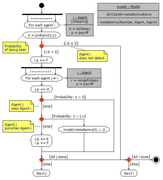
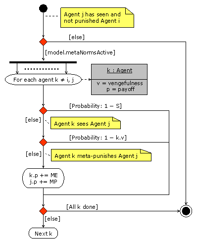
A round in this model is completed when every agent has been given exactly one opportunity to defect, and also the opportunity to observe (and maybe punish) any given defection that has taken place in the round. Figures 1 and 2 show the UML activity diagram of one round.

Figure 1
Figure 1. UML Activity diagram of one round in Axelrod's models[3]. The UML diagram of method metaNorms(Number, Agent, Agent), which does nothing in the Norms model, is provided in figure 2.

Figure 2
Figure 2. UML activity diagram of the method metaNorms(Number, Agent, Agent) of the object model. This method is called in the UML activity diagram shown in figure 1. The condition metaNormsActive is false in the Norms model and true in the Metanorms model.

3.4
Four rounds constitute a generation. At the beginning of every generation the agents' payoffs are set to zero; at the end of every generation the payoff obtained by every agent in the four rounds is computed and two evolutionary forces (i.e. natural selection and mutation) come into play to replace the old generation with a brand new one:
  1. The new generation is composed by the offspring of some of the agents in the previous generation. Agents in the old generation with a payoff exceeding the population average by at least one standard deviation are replicated twice (i.e. produce two offspring with the same strategy as the parent, subject to mutation); agents who are at least one standard deviation below the population average are eliminated without being replicated; and the rest of the agents are replicated once[4]. The number of agents is kept constant, but Axelrod (1986) does not specify exactly how. The particular algorithm implemented in our program consists in randomly eliminating (if there are more than 20 agents) or replicating (if there are fewer than 20 agents) as many agents as needed to bring the number of agents back to 20.
  2. Whenever a bitstring is replicated (which happens twice every time an agent is replicated), every bit has a certain probability to be flipped (MutationRate = 0.01).

3.5
Using this model, Axelrod (1986) comes to the conclusion that simulations should spend most of the time in states[5] of very high Boldness and very low Vengefulness. Intuitively, such states correspond to situations where the norm has collapsed.

The Metanorms Model

3.6
Having concluded that the norm to cooperate collapses in the previous model, Axelrod investigated the role of metanorms as a way of enforcing norms. The metanorm dictates that one must punish those who do not follow the norm (i.e. those who do not punish observed defectors). However, someone who does not punish an observed defector might not be caught. In the Metanorms game, the chance of being seen not punishing a defection (given that the defection has been seen) by each of the other 18 agents (excluding the defector) is the same as the chance of seeing such defection. Similarly, the propensity to punish those who do not comply with the norm (meta-punish) is the same as the propensity to punish defectors[6]. As far as payoffs are concerned, meta-punishers incur a Meta-enforcement cost (ME = -2) every time they Meta-punish (MP = -9) someone who has not punished an observed defector. Figures 1 and 2 show the UML activity diagram of one round in the Metanorms model.

3.7
Using this model, Axelrod (1986, p. 1102) argues that "the metanorms game can prevent defections if the initial conditions are favourable enough".

Table 1: Summary of Parameter Values Used by Axelrod

PARAMETERAXELROD'S VALUE
Number of Agents20
Number of Rounds per Generation4
Mutation RateMutationRate = 0.01
Temptation payoffT = 3
Hurt payoffH = -1
Enforcement payoffE = -2
Punishment payoffP = -9
Meta-Enforcement payoffME = -2
Meta-Punishment payoffMP = -9

* Method

4.1
In this paper we have used the following three tools:
  1. Computer models. We have re-implemented Axelrod's models in Java 2 using RePast 2.2 (Collier 2003), and added extra functionality to our programs so we can relax several assumptions made in Axelrod's models. The source code is available online together with a user guide at http://www.insisoc.org/metanorms under the GNU General Public Licence. An applet of our model, with which every experiment presented in this paper can be conducted, can be found in Appendix A. Using our computer models, we have been able to perform the following tasks:
    1. Replicate Axelrod's experiments using our computer models that fully comply with the specifications outlined in his paper. This exercise was conducted to study the potential presence of ambiguities and artefacts in the process of translating the model described in the paper into computer code (e.g. is the description in the paper sufficient to implement the model? Could there be implementation mistakes?, see e.g. Rouchier (2003) and Edmonds and Hales (2003b)), look for artefacts in the process of running the program (e.g. could the results be dependent on the modelling paradigm (Moss, Edmonds and Wallis 1997), programming language, or hardware platform used?), and assess the process by which the results have been analysed and conclusions derived (e.g. do the results change when the program is run for longer?).
    2. Conduct an adequate exploration of the parameter space and study the sensitivity of the model. One major disadvantage of using computer simulation is that a single run does not provide any information on the robustness of the results obtained or on the scope of the conclusions derived from them. In order to establish the scope of the conclusions derived from a simulation model it is necessary to determine the parameter range where the conclusions are invariant.
    3. Experiment with alternative models which address the relevant research question (e.g. can metanorms promote cooperation?) just as well (Edmonds and Hales 2003a). It is often the case that an agent-based model instantiates a more general conceptual model that could embrace different implementations equally well (see Cioffi-Revilla (2002) for examples of how to find possible variations). Only those conclusions which are not falsified by any of the conceptually equivalent models will be valid for the conceptual model.
  2. Mathematical analysis of the computer models. Defining a state of the system as a certain particularisation of every agent's strategy, it can be shown that both the Norms model and the Metanorms model are irreducible positive recurrent and aperiodic discrete-time finite Markov chains (with 6420 possible states)[7]. This observation enables us to say that the probability of finding the system in each of its states in the long run[8] is unique (i.e. initial conditions are immaterial) and non-zero (Theorems 3.7 and 3.15 in Kulkarni (1995). Although calculating such probabilities is infeasible, we can estimate them using the computer models.
  3. Mathematical abstractions of the computer models. We have developed one mathematical abstraction for each of the two games (the Norms game and the Metanorms game) in which we study every agent's expected payoff in any given state. These mathematical abstractions do not correspond in a one-to-one way with the specifications outlined in the previous section. They are simpler, more abstract models which are amenable to mathematical analysis and graphical representation. In particular, our mathematical models abstract the details of the evolutionary process (the genetic algorithm) and assume continuity of agents' properties (as opposed to the discrete bitstrings). The mathematical abstractions are used to suggest areas of stability and basins of attraction in the computer models, to clarify their crucial assumptions, to assess their sensitivity to parameters, and to illustrate graphically the expected dynamics of the system. Because these abstractions do not exactly correspond to the computer models, any results suggested by these mathematical abstractions are always checked by simulation. Using one model as a post-hoc summary or abstraction of another model's results to enable more powerful techniques to be applied is a very useful technique highlighted by Hales, Rouchier and Edmonds (2003).

* The Norms Model: Results and Discussion

5.1
Using the Norms model, Axelrod (1986) reports results from 5 runs consisting of 100 generations each. Even though the simulation results are not conclusive at all (i.e. they show three completely different possible outcomes), Axelrod comes to the correct conclusion that the simulations should spend most of the time in states of very high Boldness and very low Vengefulness (norm collapse) in the long term. In this section we provide a series of arguments that corroborate his conclusion.

5.2
We start by using the mathematical abstraction of the computer model. Without making any simplifying assumption so far, we can say that an agent i, with boldness bi and vengefulness vi obtains the following payoff in one round:

Equation 1 (1)

where T, H, E, P are the payoffs mentioned in the description of the model,
n is the number of agents, and

Equation 1 legend

Thus the expected payoff of agent i in one round is:

Equation 2 (2)

5.3
We define now a concept of point stability that we call Evolutionary Stable State (ESS), and which is inspired in the ideas put forward by Maynard Smith and Price (1973) and developed by Weibull (1995) and Colman (1995). An ESS is a state (determined by every agent's Boldness and Vengefulness) where:
  1. every agent in the population Θ receives the same expected payoff (so evolutionary selection pressures will not lead the system away from the state),

    Equation

  2. any single (mutant) agent m who changes its strategy (let bm be its new Boldness and vm its new Vengefulness) gets a strictly lower expected payoff than any of the other agents in the incumbent population I ≡ Θ-{m} (so if one single mutation occurs[9], the mutant agent will not be able to invade the population),

    Equation

  3. and after any single (mutant) agent m has changed its strategy, all the other agents in the incumbent population I get the same expected payoff (so a single mutant cannot distort the composition of the population except maybe by random drift).

    Equation

5.4
The three conditions above provide strong restrictions for stability in the dynamics of the model; however they are not sufficient to guarantee in the general case that, if they are fulfilled in a certain state, the system will tend to move back to such a state after one single mutation occurs. If the three conditions prevail in a certain state we know that any mutant will (be expected to) be removed from the game[10], but we cannot tell which specific agent will be replicated twice. Such replication could potentially alter the composition of the original population. Nevertheless, in the particular cases where every agent in the population is following the same strategy, the three conditions above are enough to guarantee that the system will be resistant to one single mutation[11] (in terms of expected payoffs and assuming any of the selection mechanisms studied in this paper). We will see later that in both Axelrod's models all ESSs are states where every agent is following the same strategy, so all of them are indeed resistant to one mutation.

5.5
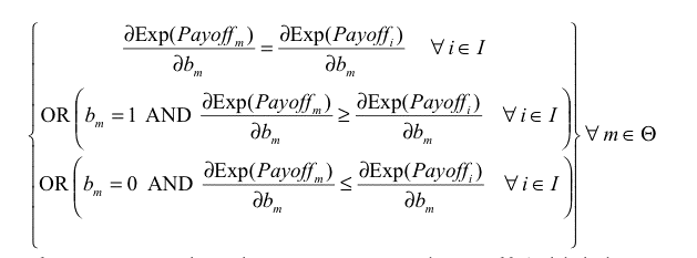
If, at this point, we assume continuity of agents' properties, we can write a necessary condition for a state to be evolutionary stable. Let m be an arbitrary (potential mutant) agent in a given population of agents Θ, and let bm be its boldness and vm its vengefulness. Let I be the set of (incumbent) agents in the population Θ excluding m. Then equation (3) is a necessary condition for the population of agents being an ESS.

Equation 3 (3)

If every agent has the same expected payoff (which is a necessary condition for ESS) and eq. (3) does not hold for some m, i, the potential mutant m could get a differential advantage over incumbent agent i by changing its Boldness bm , meaning that the state under study would not be evolutionary stable. As an example, if we find some m, i such that

Equation

then agent m could get a higher payoff than agent i by increasing its boldness bm , and condition b) in the definition of ESS would not apply. Similarly, we obtain another necessary condition substituting vm for bm in eq. (3).
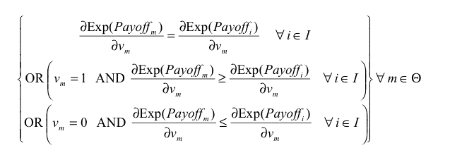
Equation 4 (4)

5.6
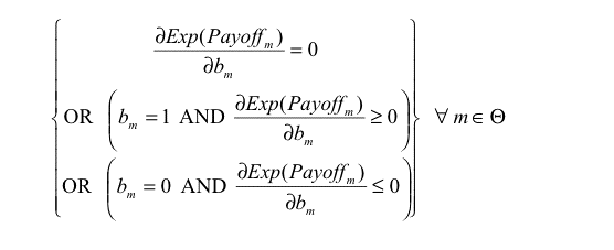
It is interesting to see how in general there is no direct relationship between the concept of evolutionary stability as defined above and the Nash equilibrium concept. Evolution is about relative payoffs, but Nash is about absolute payoffs. A necessary condition to be in Nash equilibrium would be, e.g.:

Equation

5.7
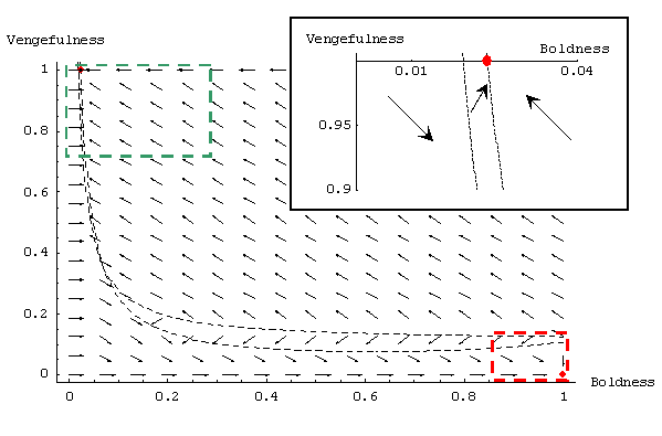
In appendix B, we use equations (3) and (4) to demonstrate that the only ESS in the Norms game (assuming continuity and using Axelrod's parameters) is the state of total norm collapse (bi = 1, vi = 0 for all i)[12]. Here, we use these equations to draw figure 3, which illustrates the expected dynamics of the system under the assumption that every agent has the same properties (bi = B, vi = V for all i). States where every agent has the same properties will be called homogeneous. Figure 3 has been drawn according to the following procedure: the arrow departing from a certain homogeneous state (B, V) has horizontal component if and only if the condition in eq. (3) is false in such a state. In that case, the horizontal component is positive if

Equation

and negative otherwise. The vertical component is worked out in a similar way but using eq. (4) instead. Only vertical lines, horizontal lines, and the four main diagonals are considered. If both equations (3) and (4) are true then a red point is drawn.
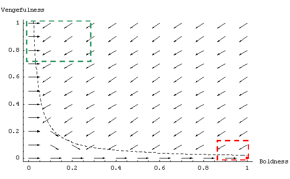
Figure 3
Figure 3. Graph showing the expected dynamics in the Norms model, using Axelrod's parameter values, and assuming continuity and homogeneity of agents' properties. The procedure used to create this graph is explained in the text. The dashed squares represent the states of norm establishment (green, top-left) and norm collapse (red, bottom-right) as defined in the text below. The red point is the only ESS. The black dashed line is the boundary that separates the region of left-pointing arrows and the region of right-pointing arrows.

5.8
As an example, imagine that in a certain state (B, V) where B ≠ 1 and V ≠ 0 we observe that:

Equation

We would then draw a diagonal arrow pointing towards greater Boldness and less Vengefulness, since a mutant with greater Boldness and less Vengefulness than the (homogeneous) population could invade it (e.g. B = 0.1, V = 0.1).

5.9
Figures constructed in this way provide an approximate picture of the expected dynamics of the system, and they can also be extremely useful to suggest new simulation experiments to run (as we will see in the next section). However, we must bear in mind that they are mathematical abstractions of the computer model, so they can also be misleading. For instance, even though figure 3 (and equation 5, formally) shows that agents can always gain a competitive advantage by decreasing their Vengefulness in any homogeneous state (unless nobody is bold), that is not necessarily the case in heterogeneous states. As an example, in a state where every agent's properties are zero except for two agents who have bi = 1 and vi = 0, each of the two bold agents would become the only agent with the highest expected payoff if it (individually) increased its vengefulness to one.

5.10
Assuming that ∀ i ∈ Θ, bi = B and vi = V (Homogeneous states)

Equation (5)

5.11
After having used a graphical representation of the system (and its assumptions) to acquire a rough idea of the expected dynamics of the simulations, we study now the behaviour of the system in the general (non-homogeneous) case by using mathematical analysis. The mathematical analysis shows that in the vast majority of states it is not advantageous in evolutionary terms to be vengeful, particularly if we increased the number of agents (eq. 6). Punishing only one agent can be advantageous for the punisher since it inflicts more pain (P) than the cost of punishing (E) (even though the punisher would also get a lower payoff!). However, if the population is minimally bold, and being vengeful means punishing too many people, the total cost of being vengeful (exclusively borne by the punisher) can be higher than each individual punishment. Therefore vengeful agents tend to be less successful. When the level of vengefulness in the population is low enough, bold agents will tend to get higher payoffs and the system will head for the state of norm collapse. So when both evolutionary forces are in place the system should spend most of its time in the neighbourhood of the only evolutionary stable state.

Equation 6 (6)

5.12
To explore further the dynamics of the model we have to resort to computer simulation. To analyse the simulation runs we define the following sets of states:

5.13
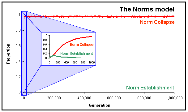
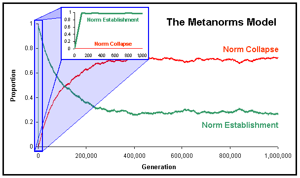
Figure 4 shows the proportion of runs (out of 1,000) where the norm has been established, and where the norm has collapsed, after a certain number of generations (up to 106) using Axelrod's Parameter values.

Figure 4
Figure 4. Proportion of runs where the norm has been established and where the norm has collapsed in the Norms model, calculated over 1,000 runs up to 106 generations using Axelrod's Parameter values. The little figure in the middle of the graph represents the first 1,000 generations zoomed.

As predicted in the previous analysis, the norm collapses almost always, as Axelrod concluded; only now the argument has been corroborated with more convincing evidence. We can also notice looking at the zoomed graph in figure 4 that it is not surprising that Axelrod found three completely different possible outcomes after having run the simulation 5 times for 100 generations.
* The Metanorms Model: Results and Discussion

6.1
Using the Metanorms model, Axelrod (1986) reports again results from 5 runs consisting of 100 generations each. In all five runs the norm is clearly established and Axelrod argues that "the metanorms game can prevent defections if the initial conditions are favourable enough" (Axelrod 1986, p. 1102). Initial conditions are indeed important for the short-term dynamics of the model. However, as explained in the method section, initial conditions are immaterial for the long-run behaviour of any of the two models under study. In this section, we investigate whether metanorms can actually prevent defections in the long run and, if so, how robust such statement is.

Replication of the Original Experiments

6.2
We replicated Axelrod's experiments but we ran many more simulations (1,000 runs, as opposed to 5) and for longer (106 generations, as opposed to 100). The results are shown in figure 5. We can see now how misleading it was to run the simulation for only 100 generations. Even though after 100 generations the norm is almost always established, as time goes by the system approaches its limiting distribution, where the norm usually collapses.

Figure 5
Figure 5. Proportion of runs where the norm has been established and where the norm has collapsed in the Metanorms model, calculated over 1,000 runs up to 106 generations using Axelrod's Parameter values. The little figure in the middle of the graph represents the first 1,000 generations zoomed.

6.3
To understand better the dynamics of the system and the sensitivity of the model we used again a mathematical abstraction of the computer model. Equation 7 shows the expected payoff for an agent i, with boldness bi and vengefulness vi. In appendix C we demonstrate that in the Metanorms game, assuming continuity, there are now two ESSs (only): one where the norm is established[13] (bi = 4/169, vi = 1 for all i), and one where the norm collapses (bi = 1, vi = 0 for all i).

Equation 7 (7)

6.4
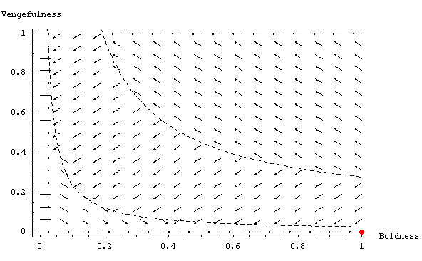
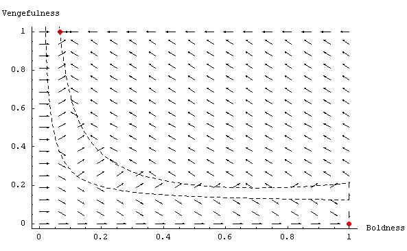
Figure 6 shows the expected dynamics of the metanorms game assuming continuity and homogeneity in agents' properties. Looking at figure 6 we find that it is not surprising that running 5 simulations for 100 rounds could mislead us to think that the norm will always be established. If the initial strategies are random, chances are that the system will move towards the ESS where the norm is established. However, the region to the left of this ESS is a nearby escape route to the ESS where the norm collapses. Intuitively, for very low levels of boldness the very few defections that occur are those that are very unlikely to be seen[14], meaning that an agent who happens to observe a defection and who does not punish it is also very unlikely to be caught. And let's face it, in this model the only reason for which agents may punish defectors is to avoid being meta-punished[15]. So when defections are hard to see, not punishing pays off because it is very unlikely that the non-punisher will be caught. Thus being vengeful is disadvantageous, and forgiving agents gain a competitive advantage. As the level of vengefulness decreases, the level of boldness below which it is advantageous not to be vengeful increases, since people meta-punish less than before (vengefulness is both the propensity to punish and to meta-punish). Agents then start to be less and less vengeful, and consequently bolder and bolder, so the norm eventually collapses.

Figure 6
Figure 6. Graph showing the expected dynamics in the Metanorms model, using Axelrod's parameter values, and assuming continuity and homogeneity of agents' properties. Red points are ESS. The dashed black lines are boundaries between regions where every arrow is pointing in the same direction. This figure has been drawn following the same procedure as in figure 3.

6.5
The study of the limiting behaviour in formal models of social systems raises some questions. It could reasonably be argued that the fundamental structure of many social processes is so ever-changing that studying the limiting behaviour of one single model with a fixed structure is often virtually irrelevant. Such a statement can be valid in some cases, but there are also several counterarguments for it:
  1. In many models of social processes (e.g. the models in this paper) the nature of the interactions under study is not defined in a specific and definite way, so it is not straightforward to determine how many time-steps in the model correspond to the short/long-term behaviour of the social system investigated.
  2. The sorts of conclusions that can be drawn by studying the short-term behaviour of a system are fundamentally different from those which can be drawn by analysing its long-term dynamics. For example, examining the short-term behaviour of Axelrod's Metanorms model we can investigate whether metanorms can delay the potential collapse of a norm or not - a question that hardly requires any modelling to answer. However, if we want to explore whether metanorms can sustainably prevent the collapse of a norm, then we need to analyse the long-term behaviour of the model.
  3. Finally, it is often the case that we cannot anticipate the significance of studying the long-term behaviour of a model before undertaking a thorough analysis of its long-run dynamics.
The experiments conducted in the next sections will allow us to draw conclusions even for the short term, but they will all be conducted for many thousands of periods to ensure the validity of our conclusions.

Some Exploration of the Parameter Space

6.6
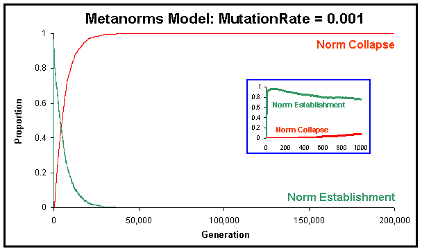
One reason for which the transition towards the set of states where the norm collapses is so slow in the Metanorms model, and for which such set is not very stable (the set is indeed sometimes abandoned), is the high mutation rate used by Axelrod. Such a high mutation rate does not allow the system to move widely by random drift after a single mutation takes place and before the next mutation occurs (this is explained in detail later). Using a lower mutation rate (MutationRate = 0.001, for which we can expect one mutation approximately every 8 generations) the system reaches the states of norm collapse much more quickly and that set is much more stable. Results are shown in figure 7.

Figure 7
Figure 7. Proportion of runs where the norm has been established and where the norm has collapsed in the Metanorms model, calculated over 1,000 runs up to 2·105 generations, with MutationRate equal to 0.001 and the rest of the parameter values equal to Axelrod's.

6.7
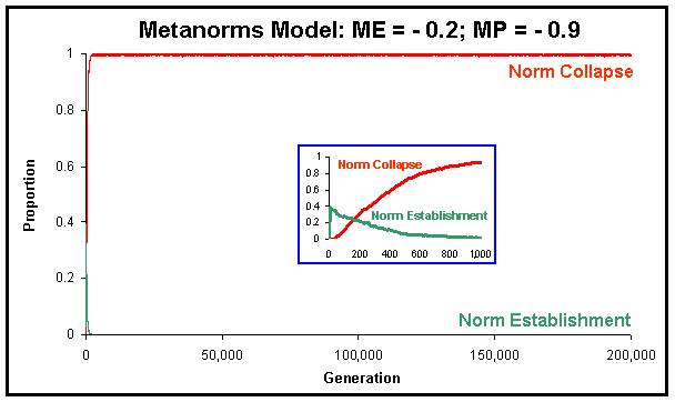
Another reason for which Axelrod's simulation results turned out to be so misleading is the extreme payoff structure that he used. In every round, agents might get the Temptation payoff at most once (benefit = 3), but they can be punished for being bold up to 19 times (with a total cost of 171) and they can be meta-punished for not being vengeful up to 342 times (with a total cost of 3078)! As an example, we show here how slightly altering the metanorm-related payoffs can significantly change the dynamics of the system. Assume that we divide both the Meta-enforcement cost and the Meta-punishment payoff by 10, leaving their ratio untouched (ME = -0.2; MP = -0.9). Such adjustments should actually give us a more realistic model: as Yamagishi and Takahashi (1994) put it: "if someone is late for a meeting you may grumble at him, but you would seldom grumble at your colleagues for not complaining to the late comer", certainly not with the same intensity! Figure 8 shows how if we use the modified payoffs the area of stability where the norm is established is not there anymore, suggesting that the transition to the states of norm collapse will be much quicker.

Figure 8
Figure 8. Graph showing the expected dynamics in the Metanorms model, with ME = -0.2; MP = -0.9 (the rest of parameter values equal to Axelrod's), and assuming continuity and homogeneity of agents' properties. The dashed black lines are boundaries between regions where every arrow is pointing in the same direction.

6.8
The simulation runs corroborate our speculations. As we can see in figure 9, the norm quickly collapses and such state is sustained in the long term. Axelrod's conclusions are reversed if we use (what in our opinion are) more realistic payoffs.

Figure 9
Figure 9. Proportion of runs where the norm has been established and where the norm has collapsed in the Metanorms model, calculated over 1,000 runs up to 2 ·105 generations, with ME = -0.2, and MP = -0.9 (the rest of parameter values equal to Axelrod's).

6.9
The mathematical abstraction of the computer model was also used to uncover a very counterintuitive feature of the original model. Strange as it may appear, the mathematical analysis suggests that increasing the magnitude of the Temptation payoff or decreasing the magnitude of the Punishment payoff will increase the chances that the norm is established. Figure 10 shows the expected dynamics when Temptation = 10. The ESS where the norm is established (bi = 11/169, vi = 1 for all i) is now surrounded by a larger basin of attraction, suggesting that the set of states where the norm is established will be more stable.

Figure 10
Figure 10. Graph showing the expected dynamics in the Metanorms model, with T = 10 (the rest of parameter values equal to Axelrod's) and assuming continuity and homogeneity of agents' properties. The dashed black lines are boundaries between regions where every arrow is pointing in the same direction.

6.10
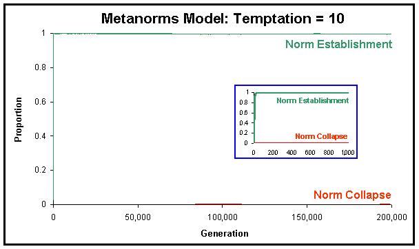
We decided to test the hypothesis that a greater Temptation payoff can increase the chances that the norm is established using our computer model. The results obtained, which are shown in figure 11, are unambiguous: the norm is clearly established in almost all runs. The reason for that is that a higher Temptation[16] means that the level of optimum boldness (in evolutionary terms) in any given situation is higher than before (e.g. assuming vi = 1 for all i, it is now b = 11/169, as opposed to 4/169). As we explained before, in the previous case the system would abandon the states where the norm is established because the level of boldness in the population was so low that agents who did not punish defectors were rarely caught. However, in this case the optimum level of boldness is not so low, so agents who do not punish defectors are more likely to be observed and meta-punished. Because of this, a very high level of vengefulness is preserved. This basically means that in the presence of metanorms, it might be easier to enforce norms which people have higher incentives to break (i.e. which are constantly put to the test) because that gives meta-punishers more opportunities to exert their power. However it is also clear that this argument requires a strong link between the propensity to punish and the propensity to meta-punish. Without such a link it seems unlikely that the norm could be established in the long-term in any case, since strategies that follow the norm without incurring the costs of enforcing it would gain a differential advantage over those that enforce it.

Figure 11
Figure 11. Proportion of runs where the norm has been established and where the norm has collapsed in the Metanorms model, calculated over 1,000 runs up to 2·105 generations, with T = 10 (the rest of parameter values equal to Axelrod's).

Other Instantiations of the Same Conceptual Model

6.11
We also wanted to test the robustness of Axelrod's conclusions using similar computer models which are, in our opinion, equally valid instantiations of the conceptual model that (we believe) Axelrod had in mind[17]. In particular, we implemented three other evolutionary selection mechanisms apart from the one Axelrod used. In all four selection mechanisms the most successful agents at a particular time have the best chance of being replicated in the following generation, which is what we believe the conceptual model would specify. The new selection mechanisms are the following:
  1. Random tournament. This method involves selecting two agents from the population at random and replicating the one with the higher payoff for the next generation. In case of tie, one of them is selected at random. This process is repeated 20 times to keep the number of agents constant.
  2. Roulette wheel. This method involves calculating every agent's fitness, which is equal to their payoff minus the minimum payoff obtained in the generation. Agents are then given a probability of being replicated (in each of the 20 replications) that is directly proportionate to their fitness[18].
  3. Average selection. Using this method, agents with a payoff greater than or equal to the population average are replicated twice; and agents who are below the population average are eliminated. The number of agents is then kept constant by randomly eliminating/replicating as many agents as needed.

6.12
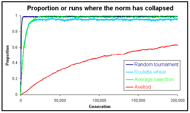
As we can see in figure 12 the results obtained in the Metanorms game vary substantially depending on the selection mechanism used. This is so particularly in the short term but also in the long term (figure 5 shows the level at which Axelrod's series becomes stable). If, for instance, random tournament is chosen, the states where the norm has collapsed are quickly reached and our experiments indicate that the long-run probability of finding the system in such states is very close to one.

Figure 12
Figure 12. Proportion of runs where the norm has collapsed in the Metanorms model, calculated over 1,000 runs up to 2·105 generations, for different selection mechanisms and using Axelrod's parameter values.

6.13
Understanding why the three additional selection mechanisms explored here result in dynamics significantly different from those that emerge when using Axelrod's selection mechanism required an in-depth analysis of individual simulation runs. The basic idea is that Axelrod's algorithm makes very difficult the transition from states where the norm is established to states where the norm has collapsed.

6.14
At the beginning of a simulation, when initial conditions are random, evolutionary forces usually push the system towards the ESS characterised by very low boldness and very high vengefulness (norm establishment), as shown in fig. 6. In these states the payoff of every agent is often exactly the same, since defections are extremely rare. This is a curious situation in which, due to the very low level of boldness, the particular value of agents' vengefulness does not actually have any influence in the dynamics of the system, since defections do not occur. While this situation (i.e. no defections) prevails, the level of vengefulness may vary, not only because of mutations, but also and more importantly, because even when every individual has the same payoff and in the absence of mutations, the genetic pool of the population can change by random drift. Agents' vengefulness may vary before a defection takes place to such an extent that when defections actually occur and selection pressures come into force, the aggregate vengefulness is so low that selection forces push the system towards the other ESS - the state of norm collapse.

6.15
How likely the escape from the ESS where the norm is established is depends on the mutation rate (i.e. the lower the mutation rate the longer the system can move by random drift in between consecutive mutations) and on how widely the system can move in one time-step (i.e. the more extensively it can move, the easier it will be to reach states of low vengefulness by random drift in few time-steps). If the mutation rate is high, the probability that defections will not occur in several consecutive time-steps is low, and when defections occur near the ESS of norm establishment, selection forces push the system back to the ESS (this explains the behaviour observed in fig. 7). Likewise, if the system cannot move very widely in one time-step (i.e. the selection mechanism does not introduce much noise), it will not be able to escape the basin of attraction of the ESS by random drift (i.e. before selection pressures act on the system and take it back to the ESS).

6.16
The three additional selection mechanisms explored here are substantially noisier than Axelrod's, thus for the three of them and given a certain mutation rate, the system can move more widely by random drift, and therefore it can more easily escape the basin of attraction of the ESS where the norm is established.

* Conclusions

7.1
This paper has provided evidence showing that the results reported by Axelrod (1986) are not as reliable as one would desire. We can obtain the opposite results by running the model for longer, by using other mutation rates, by modifying the payoffs slightly, or by using alternative selection mechanisms. These findings should not be understood as a critique of Axelrod's work, which was developed when the computational power required to undertake a thorough analysis of his model was simply not available, but as a clear illustration of the necessity to revisit and replicate our models in order to clarify the boundaries of validity of our conclusions (see Edmonds and Hales (2003b) for another striking example). As Axelrod himself claims:
Replication is one of the hallmarks of cumulative science. It is needed to confirm whether the claimed results of a given simulation are reliable in the sense that they can be reproduced by someone starting from scratch. Without this confirmation, it is possible that some published results are simply mistaken due to programming errors, misrepresentation of what was actually simulated, or errors in analysing or reporting the results. Replication can also be useful for testing the robustness of inferences from models. (Axelrod 1997b)

7.2
This paper has not only illustrated the significance of replication but it has also highlighted some best practice guidelines that agent-based modellers could find useful when developing their own models. In particular we have shown the importance of:
  1. Running simulations with stochastic components several times for several periods, so we can study not only how the system can behave but also how it usually behaves.
  2. Exploring thoroughly the parameter space and analysing the model sensitivity to its parameters.
  3. Complementing simulation with analytical work.
  4. Being aware of the scope of our computer models and of the conclusions obtained with them. The computer model is often only one of many possible instantiations of a more general conceptual model. Therefore the conclusions obtained with the computer model do not necessarily apply to the conceptual model.

7.3
The importance of the previous points has been previously exposed by authors like Gotts et al. (Gotts, Polhill and Law 2003; Gotts, Polhill and Adam 2003), and Edmonds and Hales (2003a; 2003b); the work presented in this paper strongly corroborates these authors' arguments.


* Acknowledgements

This work is funded by the Scottish Executive Environment and Rural Affairs Department, by the Junta de Castilla y León Grant Ref.: VA034/04 and by the MCyT (Spain) through the Project DPI2004-06590. We would also like to thank Gary Polhill for some advice and some programming work and the anonymous reviewers for their helpful suggestions. This paper was first presented at the 2nd ESSA Conference, 16-19 Sept 2004, Valladolid, Spain.


* Notes

1For an agent A, strategy S*A is strictly dominant if for each feasible combination of the other players' strategies, A's payoff from playing S*A is strictly more than A's payoff from playing any other strategy.

2An equilibrium is deficient if there exists another outcome which is preferred by every player.

3Arrows with solid lines represent flow of program control from the start (black circle) to the end (black circle with concentric white ring). Immediately below the top-most arrow there is a thick horizontal line, which denotes a concurring process. The dotted horizontal line between two vertical arrows departing from the same concurrent process (thick) line indicates many objects (in this case, agents) engaged in the same activity (Polhill, Izquierdo, and Gotts 2005a). Arrows with dashed lines are object flows, indicating the involvement of an object in a particular action. Objects are represented in grey boxes divided into possibly three sections. The top-most section shows the name of the object (e.g. i) and the class it belongs to (e.g. Agent), underlined and separated by a colon, with the state optionally in square brackets underneath (e.g. [stepping]). The second section in a grey box shows certain instance variables of the object; and the bottom-most section, which appears optionally, shows methods to which the object can respond (e.g. metanorms(Number, Agent, Agent)). The type of each of the arguments of a method is written between brackets after the name of the method. Comments are indicated in yellow boxes with a folded down corner, and connected by a dashed line without an arrowhead to the item with which they are associated. Red diamonds represent decision points, with one out-flowing arrow labelled with text in square brackets indicating the condition under which that branch is used, and the other out-flowing arrow indicating the 'else' branch. When the condition is of the form [Probability: x], the associated branch is followed with probability x.

4This description of the selection algorithm is ambiguous when every agent in a generation happens to obtain the same payoff. In that case, in our particular re-implementation of the model, every agent is replicated twice, and then half of the newly created agents are randomly eliminated to keep the number of agents constant. Proceeding in a different way when every agent has the same payoff can alter the long-term results significantly.

5The term 'state' denotes here a certain particularisation of every agent's strategy.

6Yamagishi and Takahashi (1994) use a model similar to Axelrod's, but propose a linkage between cooperation (not being bold) and vengefulness.

7The demonstration of this statement is simple when one realises that the mutation operator guarantees that it is possible to go from any state to any other state in one single step.

8This is also the long-run fraction of the time that the system spends in each of its states.

9By 'one single mutation', we refer to any change in one single agent's strategy, not a single flip of a bit.

10This is true for the selection mechanism used by Axelrod, and also for three other selection mechanisms that we explore in a later section.

11In other words, if every agent is following the same strategy in an Evolutionary Stable State as defined above, we can confirm that such strategy is evolutionary stable as understood in the literature (a strategy with the property that if most members of the population adopt it, no mutant strategy can invade the population by natural selection (Maynard Smith and Price 1973)).

12Since every agent is following the same strategy in this state, we can guarantee that this ESS is resistant to one single mutation in terms of expected payoffs.

13This ESS is not a Nash equilibrium.

14Remember that agents defect if and only if their boldness is higher than the probability of being seen.

15Interestingly enough, recent research suggests that people genuinely enjoy punishing others who have done something wrong (de Quervain et al. 2004).

16A lower Punishment yields very similar results, and the reasoning is the same.

17A similar approach is followed by Takadama et al. (2003), Kluver and Stoica (2003), and by Edmonds and Hales (2003a). Takadama et al. (2003) propose a cross-element validation method to validate computational models by investigating whether several models can produce the same results after changing an element in the agent architecture. Specifically they study the effect of different learning mechanisms in the bargaining game model. Similarly, Klüver and Stoica (2003) compare different adaptive algorithms over one single domain. Edmonds and Hales (2003a) compare three different evolutionary selection mechanisms, just as we have done here.

18If all agents happen to have the same payoff then random tournament is applied.


* References

ARTHUR B, Durlauf S and Lane D (1997) The Economy as an Evolving Complex System II. Reading, Massachusets.: Addison-Wesley.

AXELROD R M (1986) An Evolutionary Approach to Norms. American Political Science Review, 80 (4), pp. 1095-1111

AXELROD R M (1997a) The complexity of cooperation. Agent-based models of competition and collaboration. Princeton, N.J: Princeton University Press.

AXELROD R M (1997b) Advancing the Art of Simulation in the Social Sciences. In Conte R, Hegselmann R, Terna P, editors. Simulating Social Phenomena (Lecture Notes in Economics and Mathematical Systems 456). Berlin: Springer-Verlag.

AXTELL R L (2000) Why Agents? On the Varied Motivations for Agents in the Social Sciences. In Macah C M, Sallach D, editors. Proceedings of the Workshop on Agent Simulation: Applications, Models, and Tools. Argonne, Illinois.: Argonne National Laboratory.

AXTELL R L, Axelrod R M, Epstein J M and Cohen M D (1996) Aligning Simulation Models: A Case Study and Results. Computational and Mathematical Organization Theory, 1 (2), pp. 123-141

BENDOR J and Swistak P (1997) The evolutionary stability of cooperation. American Political Science Review, 91 (2), pp. 290-307

BENDOR J and Swistak P (1998) Evolutionary equilibria: Characterization theorems and their implications. Theory and Decision, 45 (2), pp. 99-159

BINMORE K (1998) Review of the book: The Complexity of Cooperation: Agent-Based Models of Competition and Collaboration, by Axelrod, R., Princeton, New Jersey: Princeton University Press, 1997. Journal of Artificial Societies and Social Simulation, 1 (1) https://www.jasss.org/1/1/review1.html.

BONABEAU E (2002) Agent-based modeling: Methods and techniques for simulating human systems. Proceedings of the National Academy of Sciences of the United States of America, 99 (2), pp. 7280-7287

BOUSQUET F and Le Page C (2004) Multi-agent simulations and ecosystem management: a review. Ecological Modelling, 176, pp. 313-332

BOYD R and Richerson P J (1992) Punishment Allows the Evolution of Cooperation (or Anything Else) in Sizable Groups. Ethology and Sociobiology, 13, pp. 171-195

BROWN D G, Page S E, Riolo R L and Rand W (2004) Agent-based and analytical modeling to evaluate the effectiveness of greenbelts. Environmental Modelling and Software, 19 (12), pp. 1097-1109

CASTELLANO C, Marsili M and Vespignani A (2000) Nonequilibrium phase transition in a model for social influence. Physical Review Letters, 85 (16), pp. 3536-3539

CIOFFI-REVILLA C (2002) Invariance and universality in social agent-based simulations. Proceedings of the National Academy of Sciences of the United States of America, 99 (3), pp. 7314-7316

COLLIER N (2003) RePast: An Extensible Framework for Agent Simulation. http://repast.sourceforge.net/

COLMAN A M (1995) Game Theory and its Applications in the Social and Biological Sciences, 2nd edition ed. Oxford, UK.: Butterworth-Heinemann.

CONTE R, Hegselmann R and Terna P (1997) Simulating Social Phenomena (Lecture Notes in Economics and Mathematical Systems 456). Berlin: Springer-Verlag.

DAWES R M (1980) Social Dilemmas. Annual Review of Psychology, 31, pp. 161-193

de QUERVAIN D J F, Fischbacher U, Treyer V, Schellhammer M, Schnyder U, Buck A, Fehr E (2004) The Neural Basis of Altruistic Punishment. Science, 305, pp. 1254-1258

DEGUCHI H (2004) Mathematical foundation for agent based social systems sciences: Reformulation of norm game by social learning dynamics. Sociological Theory and Methods, 19 (1), pp. 67-86

EDMONDS B (2001) The Use of Models - making MABS actually work. In Moss S, Davidsson P, editors. Multi-Agent-Based Simulation, Lecture Notes in Artificial Intelligence 1979. Berlin: Springer-Verlag.

EDMONDS B and Hales D (2003a) Computational Simulation as Theoretical Experiment. Centre for Policy Modelling Report, No.: 03-106 http://cfpm.org/cpmrep106.html.

EDMONDS B and Hales D (2003b) Replication, replication and replication: Some hard lessons from model alignment. Journal of Artificial Societies and Social Simulation, 6 (4) https://www.jasss.org/6/4/11.html.

EDWARDS M, Huet S, Goreaud F and Deffuant G (2003) Comparing an individual-based model of behaviour diffusion with its mean field aggregate approximation. Journal of Artificial Societies and Social Simulation, 6 (4) https://www.jasss.org/6/4/9.html.

EPSTEIN J M (1999) Agent-based computational models and generative social science. Complexity, 4 (5), pp. 41-60

GILBERT N and Conte R (1995) Artificial Societies: the Computer Simulation of Social Life. London: UCL Press.

GILBERT N and Troitzsch K (1999) Simulation for the social scientist. Buckingham: Open University Press.

GOTTS N M, Polhill J G and Adam W J (2003). Simulation and Analysis in Agent-Based Modelling of Land Use Change. Online Proceedings of the First Conference of the European Social Simulation Association, Groningen, The Netherlands, 18-21 September 2003. http://www.uni-koblenz.de/~kgt/ESSA/ESSA1/proceedings.htm

GOTTS N M, Polhill J G and Law A N R (2003) Agent-based simulation in the study of social dilemmas. Artificial Intelligence Review, 19 (1), pp. 3-92

HALES D, Rouchier J and Edmonds B (2003) Model-to-model analysis. Journal of Artificial Societies and Social Simulation, 6 (4) https://www.jasss.org/6/4/5.html.

HARE M and Deadman P (2004) Further towards a taxonomy of agent-based simulation models in environmental management. Mathematics and Computers in Simulation, 64, pp. 25-40

JANSSEN M (2002) Complexity and ecosystem management. The theory and practice of multi-agent systems. Chelteham, UK: Edward Elgar Pub.

KIM Y G (1994) Evolutionarily Stable Strategies in the Repeated Prisoners-Dilemma. Mathematical Social Sciences, 28 (3), pp. 167-197

KLEMM K, Eguiluz V M, Toral R and San Miguel M (2003) Nonequilibrium transitions in complex networks: A model of social interaction. Physical Review E, 67 (2)

KLEMM K, Eguiluz V M, Toral R and San Miguel M (2005) Globalization, polarization and cultural drift. Journal of Economic Dynamics & Control, 29 (1-2), pp. 321-334

KLUVER J and Stoica C (2003) Simulations of group dynamics with different models. Journal of Artificial Societies and Social Simulation, 6 (4) https://www.jasss.org/6/4/8.html.

KOHLER T and Gumerman G J (2000) Dynamics in human and primate societies: Agent-based modeling of social and spatial processes. New York: Oxford University Press and Santa Fe Institute.

KULKARNI V G (1995) Modelling and Analysis of Stochastic Systems. Boca Raton, Florida: Chapman & Hall/CRC.

LANSING J S (2003) Complex Adaptive Systems. Annual Review of Anthropology, 32, pp. 183-204

MAYNARD SMITH J and Price G (1973) The Logic of Animal Conflict. Nature, 246 (2), pp. 15-18

MOSS S, Edmonds B and Wallis S (1997) Validation and Verification of Computational Models with Multiple Cognitive Agents. Centre for Policy Modelling Report, No.: 97-25 http://cfpm.org/cpmrep25.html.

POLHILL J G, Izquierdo L R and Gotts N M (2005a) The ghost in the model (and other effects of floating point arithmetic). Journal of Artificial Societies and Social Simulation, 8 (1) https://www.jasss.org/8/1/5.html.

POLHILL J G, Izquierdo L R and Gotts N M. (2005b) What every agent-based modeller should know about floating point arithmetic. Environmental Modelling & Software. In Press.

RESNICK M (1995) Turtles, Termites, and Traffic Jams: Explorations in Massively Parallel Microworlds (Complex Adaptive Systems). Cambridge, US: MIT Press.

ROUCHIER J (2003) Re-implementation of a multi-agent model aimed at sustaining experimental economic research: The case of simulations with emerging speculation. Journal of Artificial Societies and Social Simulation, 6 (4) https://www.jasss.org/6/4/7.html.

SULEIMAN R, Troitzsch K G and Gilbert N (2000) Tools and Techniques for Social Science Simulation. Heidelberg, New York: Physica-Verlag.

TAKADAMA K, Suematsu Y L, Sugimoto N, Nawa N E and Shimohara K (2003) Cross-element validation in multiagent-based simulation: Switching learning mechanisms in agents. Journal of Artificial Societies and Social Simulation, 6 (4) https://www.jasss.org/6/4/6.html.

TESFATSION L (2002) Agent-based computational economics: Growing economies from the bottom up. Artificial Life, 8 (1), pp. 55-82

VILONE D, Vespignani A and Castellano C (2002) Ordering phase transition in the one-dimensional Axelrod model. European Physical Journal B, 30 (3), pp. 399-406

WEIBULL J W (1995) Evolutionary Game Theory. Cambridge, MA: MIT Press.

YAMAGISHI T and Takahashi N (1994) Evolution of Norms without Metanorms. In Schulz U, Albers W, Mueller U, editors. Social Dilemmas and Cooperation. Berlin: Springer-Verlag.

----

ButtonReturn to Contents of this issue

© Copyright Journal of Artificial Societies and Social Simulation, [2005]