No Free Lunch when Estimating Simulation Parameters

University of Oxford, United Kingdom
Journal of Artificial
Societies and Social Simulation 24 (2) 7
<https://jasss.soc.surrey.ac.uk/24/2/7.html>
DOI: 10.18564/jasss.4572
Received: 03-Feb-2020 Accepted: 22-Mar-2021 Published: 31-Mar-2021
Abstract
In this paper, we have estimated the parameters of 41 simulation models to find which of 9 estimation algorithms performs better. Unfortunately, no single algorithm was the best for all or even most of the models. Rather, five main results emerge from this research. First, each algorithm was the best estimator for at least one parameter. Second, the best estimation algorithm varied not only between models but even between parameters of the same model. Third, each estimation algorithm failed to estimate at least one identifiable parameter. Fourth, choosing the right algorithm improved estimation performance by more than quadrupling the number of model runs. Fifth, half of the agent-based models tested could not be fully identified. We therefore argue that the testing performed here should be done in other applied work and to facilitate this we would like to share the R package 'freelunch'.Introduction
Comparing estimation algorithms provides no winner
A mathematical model is a set of causal mechanisms connecting numerical variables. These mechanisms may depend on one or more parameters; some can be readily observed while many cannot. Because un-observed parameters affect the model output, it may be possible to identify their value by comparing the model output against what actually occurs in the data. Estimation is this process of identifying parameters by comparing model output to data. Many estimation algorithms for simulation models have emerged over the past ten years (for a general review see Hartig et al. 2011; for an agent-based review see Thiele et al. 2014; for agent-based models in economics see Fagiolo et al. 2019; Platt 2020).
There are three limitations to current estimation literature. First, papers that introduce new estimation algorithms tend to showcase their performance on few idiosyncratic examples so that comparisons across methods remain difficult. Second, reviews that compare estimation algorithms tend to be small, focusing only on one field, few models and estimation algorithms. Third, existing reviews tend to mix two steps together: the processing of model outputs into useful summary statistics (or distance functions) and the actual algorithm used for estimation. The processing phase is very specific to each discipline which makes it hard to apply lessons from one paper to agent-based models in another field.
Here, we have built a more thorough comparison of nine estimation algorithms across 41 simulation models (both agent-based and not). Our original objective was to pick the best estimation algorithm so that authors could default to it without worrying about the rest of the estimation literature. Rather, we established that there is no single best algorithm: both the absolute and relative performance are context-dependent.
The best performing estimation algorithm changes not just between models but sometimes even between parameters of the same model. Worse, even though the best algorithm is context dependent, choosing the right one matters more than quadrupling the number of simulations. Worse still, for all estimation algorithms there is always at least one case where they fail entirely to estimate a parameter that at least another algorithm has identified.
This dooms the hope of there being a “best” estimation algorithm. More practically, this prevents agent-based authors from delegating to a literature review such as this one the task of picking the estimation algorithm for them. The cross-validation testing that we implement here needs to be repeated for any new model.
Critically, the same cross-validation testing that ranks algorithms can also be used to diagnose identification failures: the inability to recover the parameters’ value from data (Canova & Sala 2009; Lewbel 2019). We show that about half of the agent-based models tested have at least one unidentifiable parameter. Identification failures are common in agent-based models but identifying them provides us with clues on how to solve them or understand their causes and consequences.
The challenge of estimating agent-based models
Two factors complicate the estimation of agent-based models. First, agent-based models tend to simulate complex systems with many moving parts and parameters. Second, it is almost always impossible to identify a likelihood function for an agent-based model (the only exception we know of is Monti et al. 2020). A likelihood function is an equation connecting parameters with data and is useful to operationalize the estimation problem into a numerical maximization (change the parameters to maximize the likelihood). For simple models, we can substitute the unknown likelihood with a quasi- or pseudo-likelihood object and maximize that instead (Hooten et al. 2020 provides a good overview on this topic in the context of agent-based models). This avenue however remains too computationally expensive for most agent-based models.
Without a likelihood, the only alternative is to condense both model output and data into a set of comparable summary statistics. The challenge in agent-based models is that there is an immense number of potential summary statistics to generate from extremely heterogeneous model outputs, such as maps, histograms and time series (Lee et al. 2015 reviews the complexities of agent-based outputs). In principle having many summary statistics ought to be an advantage as we have many dimensions on which to measure the discrepancy between data and simulation. In practice however many summary statistics will provide either noisy, useless or duplicate information and degrade estimation performance.
Subject expertise can sometimes be used to select the most important summary statistics (the list of recent developments in Fagiolo et al. 2019 for example deals almost exclusively with this task) but the choice of the best summary statistics will often be arbitrary. An alternative is to start from a large set of summary statistics and then use statistical methods to pick the summaries and weigh their information to (see Carrella et al. 2020 for an agent-based model application; see Blum et al. 2013 for an approximate Bayesian computation review; Jiang et al. 2017 for a neural network approach to discover summary statistics from simulated data). Even after choosing which summary statistic to deal with however, we still need to choose the right estimation algorithm: the procedure that maps summary statistics back to the parameters that generated them.
The qualities to look for in an estimation algorithm
The theoretical literature on simulation inference, inherited from economics and in particular the indirect inference tradition (Gourieroux et al. 1993; Grazzini & Richiardi 2015; Smith 2008), is concerned with asymptotics and in particular consistency. Consistency is achieved when the estimation algorithm converges to the real value as the data used to train it (both real raw data and number of simulation runs) grows to infinity. Zhao (2011) shows that two conditions are sufficient for consistency. First, no equifinality: two different parameter inputs cannot produce the same model output. Second, once we fix a parameter input and run the model for an infinite time steps and replications, all summary statistics must converge (that is, there cannot be summary statistics that never “settle” or do so at different values for different runs).
This theoretical contribution remains largely ignored in the applied agent-based literature. There are three justifications for this. First, consistency conditions are probably violated by many agent-based models as equifinality is common (Poile & Safayeni 2016; Williams et al. 2020) and many summary statistics are either generated by non-stationary dynamics (Grazzini & Richiardi 2015) or by distributions whose sample moments do not converge, particularly power laws (Axtell 1999; LeBaron 2001). Second, it is often impossible to test whether consistency conditions are violated. Third, asymptotic results hold little appeal for applied work facing limited data and a finite computational budget. We are usually interested in the performance we can achieve for the problem at hand rather than guaranteed consistency for infinite data we will never collect.
Applied work looks rather for three qualities in an estimation algorithm. First, we want to achieve good accuracy: estimating parameters as close as possible to the ones that generated the data we observe. Second, we want to achieve good coverage: estimating the smallest range of values that includes the real parameters with the correct pre-specified probability (confidence level). Third, we want high estimation efficiency: achieving the previous two objectives with the least amount of runs since agent-based models are expensive to simulate.
The thesis of this paper is that a fourth practical quality, i.e., testing efficiency, should be prioritized instead. We should prefer estimation algorithms that can cheaply measure their own accuracy and coverage in any given context. We can test any estimation algorithm by running a simulation with known parameters, treat its output as if it was the real data and then ask the estimation algorithm to discover the parameters we started with. While the testing technique is universal, its computational costs differ between algorithms.
Why we focus exclusively on reference table algorithms
There are two main families of estimation algorithms: rejection-based and search-based algorithms. Rejection algorithms repeatedly run a model with random parameters until a stopping condition is reached. Reference table algorithms (Cornuet et al. 2008) are the subset of rejection algorithms where the stopping condition is simply to run the model a fixed amount of times.
Rejection algorithms are inefficient because many runs will produce output far from the real data. Search-based algorithms then replace random sampling with minimizing a distance function between model output and data (Calvez & Hutzler 2006; Pietzsch et al. 2020; Sisson et al. 2016). This approach increases estimation efficiency.
The estimation efficiency of search-based methods becomes a liability when testing, however. Search algorithms explore only the part of the parameter space closest to the original dataset while testing requires it to minimize the distance to many new targets. Search-based algorithms have no alternative but to restart their minimization for every new test. The computational costs of testing search-based algorithms quickly become astronomical (a point well demonstrated in Platt 2020).
Testing reference table algorithms, by contrast, involves running no new simulation. The original simulation runs were already spread out across the parameter space and the same runs used to estimate the parameters of the real dataset can be used to estimate the parameters in any new test. The advantage is even greater when we want to rank the performance of many estimation algorithms. This is because we can recycle the simulation output used to train one reference table algorithm to perform the same estimation with any other. In contrast because search-based algorithms control the trajectory of parameters fed into the model, we need to re-run the model again for each search-based algorithm we want to rank.
A numerical comparison may help. Imagine producing a testing set of 500 runs with known input parameters. We want to rank five alternative algorithms by their ability to re-discover the known parameters given a computational budget of 1,000 simulations per estimation. Testing five search-based algorithms will require us to run the simulation model 2,500,000 times: 1,000 runs for each of the five search algorithms for each of the 500 items in the testing set. Comparing five different reference table methods will require only 1,000 runs in total to produce a training dataset which will be shared across each algorithm and re-used for each item of the testing set.
Materials and Methods
Here, we define a simulation model as any function that depends on a set of parameter \(\theta\) to generate a set of summary statistics \(S(\theta)\). We are interested in the estimation problem where we observe summary statistics \(S^*\) and we want to know which parameter \(\theta^*\) most likely generated them.
We parametrized 41 simulation models (described in Section 2.5 and in the Appendix). We used nine estimation algorithms to do so (described in Section 2.9). All are “reference table” algorithms: algorithms whose only input for estimation is a table of simulation parameters \(\theta\), selected by random sampling, and the summary statistics \(S(\theta)\) they generate. We split this reference table into training and testing sets and ask each algorithm to estimate the parameters of the testing set observing only the training runs.
We wanted to measure the quality of an estimation algorithm along two dimensions: point predictions “performance” and confidence interval “coverage.” We measured point prediction performance as:
| \[\text{Performance} = 1 - \frac{ \sum_j \sqrt{\left( \theta^*_j - \hat \theta_j \right)^2}}{ \sum_j \sqrt{\left( \theta^*_j - \bar \theta \right)^2}} \] | \[(1)\] |
We defined coverage as in Raynal et al. (2019) as the percentage of times the real parameter falls within the 95% prediction intervals suggested by the estimating algorithm. The best coverage is 95%: higher generates type I errors, lower generates type II errors.
Models
We estimated the parameters of 41 separate simulation models and them either as they appeared as examples in at least another estimation paper (20 models) or because they were open source agent-based models (21 models) available on the COMSES model library (Rollins et al. 2014). We can roughly categorize these models into four groups: simple, ill posed, complicated and agent-based models. Table 1 lists them all. In the Appendix, we provide a brief description of each.
| Experiment | No. of parameters | No. of summary statistics | No. of simulations | Testing |
|---|---|---|---|---|
| \(\alpha\)-stable | 3 | 11 | 1,250 or 5,000 | 5-fold CV |
| Anasazi ABM | 4 | 28 | 1,250 or 5,000 | 5-fold CV |
| Birds ABM | 2 | 2 or 105 | 5,000 | 5-fold CV |
| Bottom-up Adaptive Macroeconomics ABM | 8 | 180 | 1,250 or 5,000 | 5-fold CV |
| Broken Line | 1 | 10 | 1,250 or 5,000 | 5-fold CV |
| Coalescence | 2 | 7 | 100,000 | Single testing set |
| COVID-19 US Masks ABM | 4 | 51 | 1,250 or 5,000 | 5-fold CV |
| Earthworm | 11 | 160 | 100,000 | Single testing set |
| Ecological Traits | 4 | 4 | 1,250 or 5,000 | 5-fold CV |
| Ebola Policy ABM | 3 | 31 | 1,250 or 5,000 | 5-fold CV |
| FishMob ABM | 5 | 104 | 1,250 or 5,000 | 5-fold CV |
| Food Supply Chain ABM | 5 | 99 | 1,250 or 5,000 | 5-fold CV |
| Ger Grouper ABM | 4 | 41 | 1,250 or 5,000 | 5-fold CV |
| \(g\)-and-\(k\) distribution | 4 | 11 | 1,250 or 5,000 | 5-fold CV |
| Governing the Commons ABM | 4 | 44 | 1,250 or 5,000 | 5-fold CV |
| Hierarchical Normal Mean | 2 | 61 | 1,250 or 5,000 | 5-fold CV |
| Intra-Organizational Bandwagon ABM | 2 | 43 | 1,250 or 5,000 | 5-fold CV |
| Insulation Activity ABM | 3 | 45 | 1,250 or 5,000 | 5-fold CV |
| Lotka-Volterra | 2 | 16 (noisy or non-noisy) | 100,000 | Single testing set |
| Locally Identifiable | 2 | 2 | 1,250 or 5,000 | 5-fold CV |
| Moving Average (2) | 2 | 2 | 1,250 or 5,000 | 5-fold CV |
| Median and MAD | 2 | 2 or 4 | 1,250 or 5,000 | 5-fold CV |
| Multilevel Selection ABM | 4 | 44 | 1,250 or 5,000 | 5-fold CV |
| \(\mu\)-\(\sigma^2\) | 2 | 2 | 10,000 | 5-fold CV |
| NIER ABM | 4 | 60 | 1,250 or 5,000 | 5-fold CV |
| Normal 25 | 2 | 25 | 1,250 or 5,000 | 5-fold CV |
| Pathogen | 4 | 11 | 200,000 | Single testing set |
| Partially Identifiable | 2 | 2 | 1,250 or 5,000 | 5-fold CV |
| Peer Review Game ABM | 5 | 77 | 1,250 or 5,000 | 5-fold CV |
| OfficeMoves ABM | 3 | 36 | 1,250 or 5,000 | 5-fold CV |
| RiskNet ABM | 4 | 40 | 1,250 or 5,000 | 5-fold CV |
| Real Business Cycle | 6 | 44 or 48 | 2,944 or 2,961 | 5-fold CV |
| Scale | 2 | 1 | 1,250 or 5,000 | 5-fold CV |
| Schelling-Sakoda Extended ABM | 3 | 77 | 1,250 or 5,000 | 5-fold CV |
| Standing Ovation ABM | 3 | 20 | 1,250 or 5,000 | 5-fold CV |
| Sugarscape ABM | 5 | 146 | 1,250 or 5,000 | 5-fold CV |
| Unidentifiable | 2 | 1 | 1,250 or 5,000 | 5-fold CV |
| Toy Model | 2 | 2 | 1,250 or 5,000 | 5-fold CV |
| Two-factor Theory ABM | 4 | 41 | 1,250 or 5,000 | 5-fold CV |
| Wilkinson | 1 | 1 | 1,250 or 5,000 | 5-fold CV |
| Wolf Sheep Predation ABM | 7 | 33 | 1,250 or 5,000 | 5-fold CV |
Simple simulation models have few parameters and summary statistics. They feature prominently in the ABC literature both as a teaching tool and to compare different algorithms. They are useful because they run quickly but they may bias comparisons towards simpler estimation algorithms.
Ill-posed simulation models face clear identification issues: the inability to recover parameters given the information we have. There are many sources of identification issues and each ill-posed model highlights one particular form. A good estimation algorithm facing an ill-posed problem should display two features. First, it should maximize the quality of our estimated parameters when the information is available but noisy (the lesser problem of “weak” identification). Second, estimation algorithm should recognize when the model cannot be identified and return wide confidence intervals, signaling estimation uncertainty.
We split complicated simulation models into two sets, agent-based models and other complicated simulations. They face similar problems: they tend to be large, involve many input parameters and summary statistics. From an estimation point of view there is no qualitative difference between the two but in practice agent-based models tend to be slower and produce more summary statistics.
Algorithms
We tested nine reference table algorithms to parametrize simulations: five are ABC (Approximate Bayesian Computation) and four are regressions-only. We ignored search-based algorithms, such as synthetic likelihood (Fasiolo & Wood 2014; Wood 2010), ABC-MCMC (Hartig et al. 2011) and Bayesian optimization (Snoek et al. 2012). We also ignored regression-only algorithms that do not generate prediction intervals such as the deep neural networks proposed in Creel (2017) and the elastic nets proposed in Carrella et al. (2018).
All reference table algorithms share a common estimation procedure. First, we ran the model “many” times and collected the random parameters we input and summary statistics the model outputs into a “reference table.” The estimation algorithm allowed us to produce a rule to generalize the information in the reference table and to go from summary statistics back to the parameters that generated them. Finally, we plugged in the real summary statistics vector \(S^*\) we observed from the data into this rule and obtained the estimated parameters.
ABC
The first algorithm we use is the simple rejection ABC (Beaumont et al. 2002; Pritchard et al. 1999). Start by ranking all training observations by their euclidean distance to the testing summary statistics \(\sum_i\left( S_i(\theta) - S^*_i \right)^2\). Let us ignore all training observations except the closest 10%. The distribution of \(\theta\) parameters from the closest training observations becomes the posterior of the estimate \(\theta^*\).
The second algorithm is the local-linear regression adjusted ABC (Beaumont et al. 2002). Weigh all training observations by an Epanechnikov kernel with bandwidth equal to Euclidean the distance between the testing summary statistics \(S^*\) and the furthest \(S(\theta)\) we would have accepted using simple rejection. Then run a local-linear regression on the weighted training set to estimate \(\theta^*\) as the predicted \(E[\theta |S(\theta)]\), using the residuals of that regression to estimate its posterior distribution.
The third algorithm, neural network ABC, inputs the same weighted training set to a feed forward neural network (Blum & Francois 2010). The approach is similar to the local-linear regression described above but the residuals are also weighted by a second regression (on the log squared residuals) to correct for heteroskedasticity.
These three algorithms are implemented in the abc package (Csilléry et al. 2012) in R. We used the package default settings for its neural networks (10 networks, 5 units in the hidden layer and weight decay randomly chosen for each network between \(0.0001\),\(0.001\) and \(0.01\)).
The fourth and fifth algorithm are semi-automatic ABC methods which “pre-process” summary statistics before applying rejection ABC (Prangle et al. 2014). More precisely, the original summary statistics \(S(\theta)\) are fed into a set linear regressions estimating \(r_i=E[\theta_i|S(\theta)]\) (one for each parameter of the model) and the values are used as summary statistics for the simple rejection ABC. The rationale is that these regressions will project the summary statistics into a space where rejection ABC performs better. We did this in two different ways here: by running first or fourth degree linear regressions in the pre-processing phase. This was done using the R package abctools (Nunes & Prangle 2015) and their default parameters: using half of the training set to run the regression and the other half to run the rejection ABC.
A feature of all ABC methods is that they are local: they remove or weight training observations differently depending on the \(S^*\) (the “real” summary statistics). This means that during cross-validation we need to retrain each ABC for each row of the testing set.
Regression only
Estimating parameters by regression is a straightforward process. We build a separate regression \(r\) for each \(\theta\) in the reference table as dependent variable using the summary statistics \(S(\theta)\) as the independent variables. We plug the real summary statistic \(S^*\) in each regression and the predicted value is the estimated parameter \(\theta^*\).
The simplest algorithm of this class is linear regression of degree one. It is linear, its output is understandable and is fast to compute. This speed permits to estimate the prediction interval of \(\theta^*\) by resampling bootstrap (Davison & Hinkley 1997): 200 bootstrap data sets are produced and the same linear regression is run on each one. From each regression \(i\), their prediction \(\beta_i S(\theta^*)\) are collected and one standardized residual \(e\) is sampled (a residual divided by the square root of one minus the hat value associated with that residual). This produces a set of 200 \(\beta_i S(\theta) + e_i\). The 95% prediction interval is then defined by 2.5 and 97.5 percentile of this set.
In practice, predictions are then distributed with the formula:
| \[r(S)+A+B\] | \[(2)\] |
A more complex algorithm that is not linear but still additive is the generalized additive model(GAM), where we regress:
| \[\hat \theta = \sum s_i(S_i(\theta))\] | \[(3)\] |
mgcv R package (Wood 2004, 2017). The bootstrap prediction interval for the linear regression was too computationally expensive to replicate with GAMs. Instead, prediction intervals are produced by assuming normal standard errors (generated by the regression itself) and by resampling residuals directly: we generate 10,000 draws of \(z(S(\theta))+\epsilon\) where \(z\) is normally distributed with standard deviation equal to regression’s standard error at \(S(\theta)\) and \(\epsilon\) was a randomly drawn residual of the original regression. The 95% prediction interval for \(\theta^*\) is then defined by 2.5 and 97.5 percentile of the generated \(z(S(\theta^*))+\epsilon\) set.
A completely non-parametric regression advocated in Raynal et al. (2019) is the random forest (Breiman 2001). This has been implemented in two ways. First, as a quantile random forest (Meinshausen 2006), using in quantregForest R package (Meinshausen 2017); prediction intervals for any simulation parameter \(\theta^*\) are the predicted 2.5 and 97.5 quantile at \(S(\theta^*)\). Second, as a regression random forest using the ranger and caret packages in R (Kuhn 2008; Wright & Ziegler 2017). For this method, we generate prediction intervals as in GAM regressions. 10,000 draws of \(z(S(\theta))+\epsilon\) are generated where \(z\) is normally distributed with standard deviation equal to the infinitesimal jackknife standard error (Wager et al. 2014) at \(S(\theta)\) and \(\epsilon\) is a resampled residual; the 2.5 and 97.5 percentile of the \(z(S(\theta^*))+\epsilon\) set is then taken as our prediction interval.
Results
Point performance
Table 2 summarizes the performance of each algorithm across all identifiable estimation problems (here defined as those where at least one algorithm achieves performance of 0.1 or above). Estimation by random forests achieves the highest average performance and the lowest regret (average distance between its performance and the highest performance in each simulation). Even so, regression random forests produce the best point predictions only for 77 out of 226 identifiable parameters. GAM regressions account for another 69 best point predictions.
Local linear regression and neural-networks are also useful in the ABC context, achieving the highest performance for 47 parameters. Local linear regressions face numerical issues when the number of summary statistics increases and they were often unable to produce any estimation. The performance of neural network ABC could be further improved by adjusting its hyper-parameters, but this would quickly accrue high computational costs. The Appendix contains a table with the performance for all parameters generated by each algorithm.
| Algorithm | # of times highest performance | Regret | Median performance |
|---|---|---|---|
| Rejection ABC | 2 | -0.518 | 0.240 |
| Semi-automatic ABC 4D | 1 | -0.256 | 0.437 |
| Semi-automatic ABC 1D | 4 | -0.310 | 0.388 |
| Local-linear ABC | 16 | -0.083 | 0.560 |
| Neural Network ABC | 33 | -0.103 | 0.502 |
| Linear Regression | 11 | -0.232 | 0.399 |
| GAM | 69 | -0.034 | 0.518 |
| Quantile Random Forest | 14 | -0.039 | 0.556 |
| Regression Random Forest | 77 | -0.009 | 0.566 |
It is important to note that the advantages of random forests become apparent only when estimating agent-based models. Simpler estimation algorithms perform just as well or better in smaller problems. This is shown in Table 3. This implies that interactions between summary statistics as well as the need to weigh them carefully matters more when estimating agent-based models than simpler simulations, justifying the additional algorithm complexity.
| Algorithm | ABM | Complicated | Ill-posed | Simple |
|---|---|---|---|---|
| Rejection ABC | 0 | 0 | 1 | 1 |
| Semi-automatic ABC 4D | 0 | 0 | 0 | 1 |
| Semi-automatic ABC 1D | 3 | 0 | 0 | 1 |
| Local-linear ABC | 1 | 3 | 1 | 11 |
| Neural Network ABC | 22 | 7 | 0 | 4 |
| Linear Regression | 3 | 0 | 4 | 4 |
| GAM | 39 | 10 | 9 | 11 |
| Quantile Random Forest | 11 | 2 | 0 | 1 |
| Regression Random Forest | 58 | 8 | 1 | 10 |
Another important qualification is that random forests tend to perform better for the parameters where maximum performance is below 0.3. This is intuitive because we expect non-linear regressions to function even when summary statistics were noisy and uninformative but it also meant that many of the parameters that were best estimated by random forests remain only barely identified (see Table 4).
| Algorithm | 0.1-0.3 | 0.3-0.5 | 0.5-0.7 | 0.7-1 |
|---|---|---|---|---|
| Linear Regression | 2 | 1 | 2 | 6 |
| Local-linear ABC | 3 | 3 | 3 | 7 |
| GAM | 10 | 7 | 20 | 32 |
| Neural Network ABC | 2 | 9 | 9 | 13 |
| Rejection ABC | 1 | 0 | 1 | 0 |
| Quantile Random Forest | 0 | 1 | 7 | 6 |
| Regression Random Forest | 23 | 9 | 26 | 19 |
| Semi-automatic ABC 1D | 1 | 3 | 0 | 0 |
| Semi-automatic ABC 4D | 0 | 0 | 1 | 0 |
Table 5 lists the number of identification failures: parameters for which the algorithm performance was below 0.1 but at least a competing algorithm achieved performance of 0.3 or above. In other words, we are tabulating cases where the parameter are identified but an estimation algorithm fails to do so. Local-linear regression struggled with the “natural mean hierarchy” simulation. Linear regression failed to estimate the \(b\) parameter from the Lotka-Volterra models, the \(\sigma\) parameter from the normal distribution and the \(A\) parameter from the ecological traits model. Random forests failed to identify \(\mu\) and \(\delta\) from the RBC macroeconomic model. GAM regressions, in spite of having often been the best estimation algorithm, failed to identify 10 parameters, all in agent-based models (particularly in “Sugarscape” and “Wolf-Sheep predation”).
Table 5 also shows mis-identifications, cases where an algorithm estimated significantly worse than using no algorithm at all (performance is below -0.2). These are particularly dangerous failures because the estimation algorithm “thinks” it has found some estimation pattern which proves to be worse than assuming white noise. Mis-identification seems to apply asymmetrically: it is more common for complicated approximate Bayesian computations and simple regressions.
| Algorithm | Identification Failures | Mis-identifications |
|---|---|---|
| Rejection ABC | 32 | 2 |
| Semi-automatic ABC 4D | 2 | 0 |
| Semi-automatic ABC 1D | 2 | 0 |
| Local-linear ABC | 9 | 8 |
| Neural Network ABC | 1 | 5 |
| Linear Regression | 13 | 17 |
| GAM | 13 | 3 |
| Quantile Random Forest | 3 | 0 |
| Regression Random Forest | 3 | 0 |
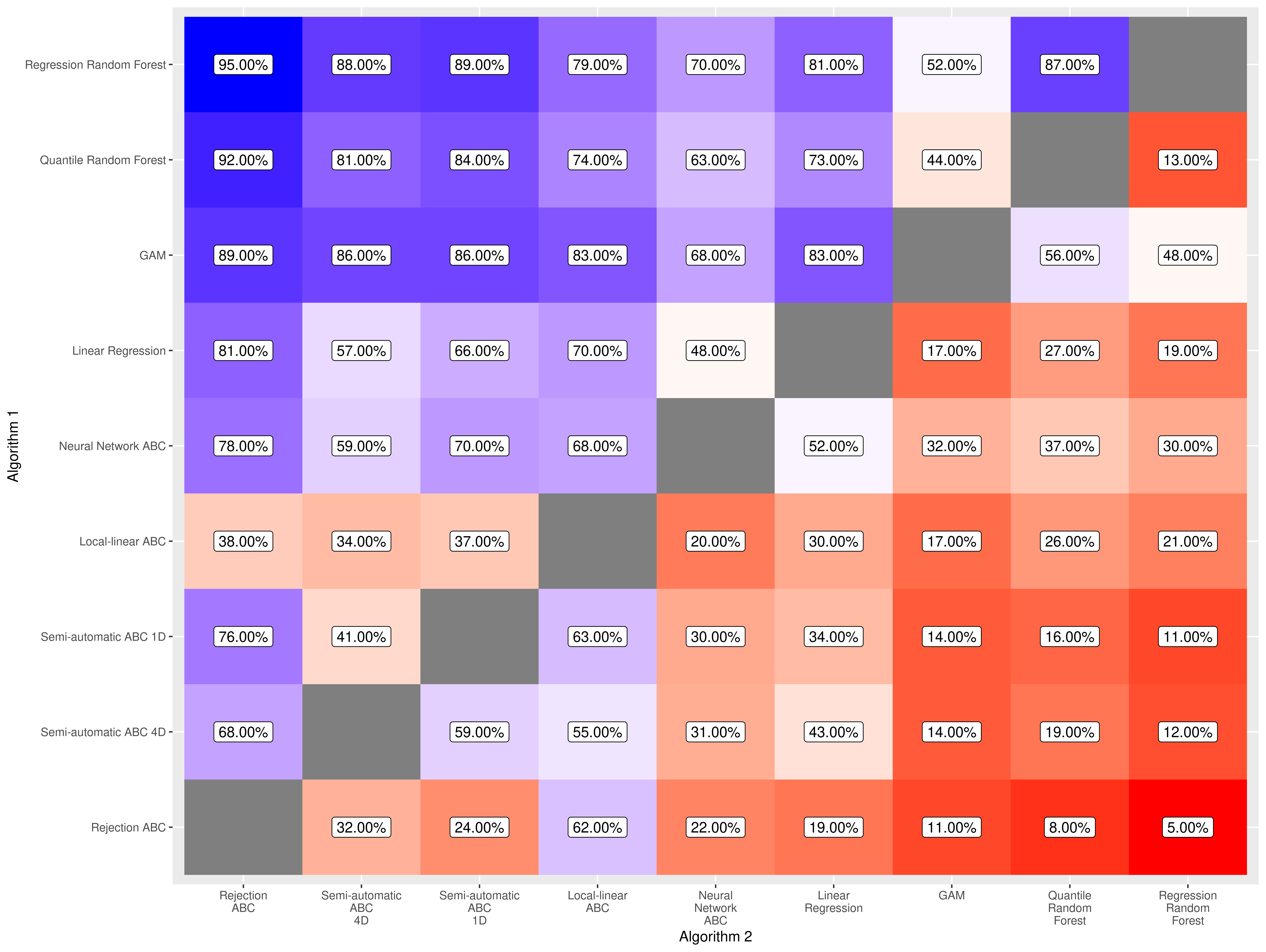
Figure 1 compares algorithms pairwise with respect to their performance. Even the “best” algorithm, random forest, has only a 52% chance of doing better than GAMs and performs worse than neural-network ABC for 30% of the parameters. The humble first degree linear regression (even after accounting for its identification failures and mis-identifications) wins more than half of the comparisons against any ABC except neural-networks.
While there was no overall winner, this does not mean that the algorithm choice is unimportant. On average, we improved point prediction performance more by choosing the right algorithm than quadrupling the training data size. To prove this point, we focus on all parameters that were estimated both with 1,250 and 5,000 training simulations. Across 237 estimated parameters, switching from the worst to the best algorithm improves point prediction performance on average by 0.323 (standard deviation of 0.248, 241 observations) and switching from median to best algorithm improves performance by 0.230 (standard deviation of 0.204, 241 observations). Quadrupling the number of training runs but using the same estimation algorithm increases performance by only 0.0370 (standard deviation of 0.0736, 812 observations).
Identification failures in agent-based models
The same approach used to rank estimation algorithms can be used to diagnose whether the model can be identified at all: if all algorithms fail to achieve cross-validation performance above a threshold then the parameter cannot be identified. Table 6 lists how many parameters we failed to identify for each agent-based model. We used two performance thresholds: “serious identification failures” were parameters where the best performance among all algorithms was below 0.1 and “identification failures” when the best performance was below 0.30. The 0.30 threshold derives from the “scale” model, the canonical example of impossible identification, which in our tests achieves maximum performance of 0.30. Ten out of 21 agent-based models have at least one serious identification failure, 14 out of 21 have at least one identification failure.
| Agent-based Model | # of parameters | # Identification Failures | # Serious Identification Failures |
|---|---|---|---|
| Anasazi | 4 | 2 | 2 |
| Bottom-up Adaptive Macroeconomics | 8 | 6 | 3 |
| Intra-Organizational Bandwagon | 2 | 1 | 1 |
| Governing the commons | 4 | 1 | 0 |
| COVID-19 US Masks | 4 | 3 | 2 |
| Earthworm | 11 | 5 | 3 |
| Ebola Policy | 3 | 1 | 1 |
| FishMob | 5 | 4 | 2 |
| Ger Grouper | 4 | 3 | 1 |
| Two-factor Theory | 4 | 0 | 0 |
| Insulation Activity | 3 | 2 | 1 |
| Multilevel Selection | 4 | 1 | 0 |
| NIER | 7 | 1 | 0 |
| Peer Review Game | 5 | 1 | 0 |
| OfficeMoves | 3 | 0 | 0 |
| RiskNet | 4 | 0 | 0 |
| Schelling-Sakoda Extended | 3 | 0 | 0 |
| Standing Ovation | 3 | 0 | 0 |
| Sugarscape | 5 | 0 | 0 |
| Food Supply Chain | 5 | 1 | 1 |
| Wolf Sheep Predation | 7 | 1 | 0 |
In applied work, identification failures will be more common than the table suggests for two reasons. First, we did not model lack of data which often reduces the quality of summary statistics. For example, in the “Intra-Organizational Bandwagon” agent-based model we assumed the ability to monitor adoption thresholds for employees, something impossible in real world applications. Second, the thresholds for failure are somewhat arbitrary and in some applied work we may require higher performance for estimation to be useful.
Because identification failure has many causes, one needs to look at each model to diagnose its source. Sometimes, we failed to estimate multiple parameters because they governed the same behaviour in ways that made them hard to separate. For example, fertility in the Anasazi model depends on both a base fertility rate and maximum fertile age and it is hard to disentangle the two by just looking at aggregate population dynamics. Sometimes, we failed to estimate parameters because their original bounds are small enough that their effects are muted: in the COVID agent-based model the parameter controlling what percentage of the population wears N95 masks varies between 0 and 5% and on its own this has no appreciable effect to the overall aggregate behaviour of the contagion. Sometimes a parameter was dominated by others: in the Ebola model the parameter describing the ability to trace cases cannot be identified because two other parameters (the effectiveness of the serum and the delay with which it is administered) matter far more to the overall aggregate dynamic. Sometimes parameters just did not have much of an impact to the model, as for example the overall standard deviation of catchability in the FishMob agent-based model.
Understanding the nature of identification failures helped us to find ways to overcome them or judge whether it is a problem at all. Disentangling multiple parameters that govern the same behaviour can be done by collecting new kinds of data or simplifying the model. Low performance of parameters with very narrow ranges is a signal of unreasonable accuracy requirements (or alternatively, low power of the data). The low performance of dominated parameters has valuable policy implications since it shows some dynamics to be less important than others to control.
The main inconvenience with testing for identification is that we need to test the performance of many estimation algorithms before being confident of the diagnosis. When one algorithm achieves low performance, it may be the algorithm’s fault rather than the model’s. Only when all algorithms achieve low performance, can we be more confident about the model not being identifiable. If our threshold for identifiability is 0.30, the smallest set of algorithms that finds all the identifiable parameters for all the examples in the paper is of size 4: random forest, GAM, neural network ABC and local-linear ABC. However, it is probable that with more examples we would expose at least one case where identification is achieved exclusively with another algorithm. In short, a good identification test will require us to test as many estimation algorithms as possible.
Coverage
To test the quality of the confidence intervals, Table 7 shows how often the real testing parameter is within the confidence intervals estimated by each algorithm. Two methods that achieved low point prediction performance, rejection ABC and linear regression, achieve best coverage rates for 35% of the parameters. This underscores how even when point prediction is difficult, a good estimation algorithm will produce confidence intervals that contain the real parameters with the pre-specified confidence level. Linear regressions have the lowest mean and median coverage error while regression-adjusted ABCs tend to produce too narrow confidence intervals.
| Algorithm | # of times most accurate | Median Coverage Error | Mean Coverage Error | # coverage below 80% | # coverage below 60% |
|---|---|---|---|---|---|
| Rejection ABC | 36 | 0.0132 | 0.0188 | 2 | 2 |
| Semi-automatic ABC 4D | 18 | 0.0169 | 0.0193 | 0 | 0 |
| Semi-automatic ABC 1D | 7 | 0.0156 | 0.0185 | 0 | 0 |
| Local-linear ABC | 4 | 0.0276 | 0.0816 | 16 | 8 |
| Neural Network ABC | 9 | 0.0929 | 0.1824 | 85 | 42 |
| Linear Regression | 64 | 0.0064 | 0.0077 | 0 | 0 |
| GAM | 72 | 0.0062 | 0.0161 | 6 | 0 |
| Quantile Random Forest | 20 | 0.0260 | 0.0298 | 5 | 0 |
| Regression Random Forest | 48 | 0.0092 | 0.0130 | 0 | 0 |
When a parameter was unidentifiable most algorithms returned very wide confidence intervals. This is a useful feature that warns the user about the poor point estimation quality. Observing confidence intervals is however not a good substitute for a full cross-validation test. This is because, as we show in Table 7, it is possible for the confidence intervals to be too small, covering only 80% or even 60% of the true parameters. In other words, sometimes estimation algorithms are mistakenly confident about their accuracy and we need a cross-validation coverage test to verify. Perversely coverage errors are more likely with algorithms that achieved high estimation performance (random forests, GAMs and neural networks).
Discussion
A simple identification testing protocol even if we are not interested in estimation
In this paper, we argued that cross-validation testing is useful to rank estimation algorithms. There are however many models where estimation is not a major concern. Models focusing on theoretical exposition, illustration or description (to use Edmonds et al. 2019 definitions) are not concerned with the true value of any specific parameter. We argue however that testing ought to be done even under these circumstances to notice identification issues.
Identification represents an important feature of the model: whether it can be fit to data at all. We claim that uncovering identification is of the same importance as sensitivity analysis and the two procedures mutually reinforce one another. An un-identifiable parameter must be tested during sensitivity analysis over a large range, since data will never narrow its value down. Vice-versa finding during sensitivity analysis that a model output is insensitive to a parameter provides an important clue to explain identification issues. Performing only sensitivity analysis and preferring models that are less sensitive creates a bias that leads us to prefer less identifiable models
Ideally, we would like to test for identification without ever running new simulations. We can do this with reference-table methods by recycling the runs used for global sensitivity analysis (Broeke et al. 2016; Ligmann-Zielinska et al. 2020; Magliocca et al. 2018). Given the results from Section 3.9, we suggest at least looking at the performance of random forests, GAMs, neural network ABC and local-linear regression ABC. If performance is below 0.30 for all, we can be relatively confident that the parameter is not identifiable.
We worry too much about efficiency and too little about testing
Many recent developments in estimation of simulations have focused on efficient search(see the various algorithms featured in Cranmer et al. (2020) review of the “frontier” of simulation-inference). While we welcome higher estimation efficiency, we think this objective is often pursued at the expense of testing efficiency.
The pursuit of estimation efficiency can be explained by the desire to build complicated models that run slowly but can still fit to data. The more efficient the estimation algorithm, the bigger our model can get and still be estimated in a given computational budget. Here, however, we highlighted the trade-off between estimation and testing efficiency. Recognizing that faster estimation comes at the price of slower testing, there is again an incentive to focus on the kind of simpler agent-based models advocated, for example, in Miller & Page (2009).
We are not claiming that search-based estimation algorithms should not be used. Given how context-dependent performance is there must be many agent-based models that will be better estimated by search-based algorithms. Our argument is that even when using a search-based algorithm we should perform a cross-validation test using reference-table methods first, take notice of the unidentified parameters and discount the value that search-based algorithms assign to them.
Estimation testing is not validation
The idea of cross-validation testing as a way to judge estimation accuracy, as well as the older statistical convergence literature it tries to replace, is premised on a lie: the existence of the mythical “real” parameters. The “real” parameters are the parameters of the “real” model that generated the data we observe. In other words, during estimation and cross-validation we are forced to assume our model to be true when we know it to be false. This is what Gelman & Shalizi (2013) calls “methodological fiction.”
Gelman & Shalizi (2013) goes on to stress that the question is not whether the model is true, but whether it is close enough to be useful. Establishing whether the model is “good enough” is the process of validation. The cross-validation tests we are advocating for here are not a validation tool but are instead part of the estimation procedure that precedes validation. Once we have an estimated model, we can test its validity through, for example, out of sample predictions or qualitative responses to shocks in ways experts find believable.
Conclusion
This paper provides two key results. First, if we are concerned primarily with the quality of point estimates, there is no substitute for trying multiple algorithms and ranking them by cross-validation. GAM and random forests provide a good starting point. Second, identification failure is common in agent-based models but can be spotted with the same cross-validation tests.
We know of no agent-based model that used cross-validation to choose how to estimate its parameters (with the exception of the comparison between ABC MCMC and simulated minimum distance in Grazzini et al. 2017). The common approach seems to be to pick one estimation algorithm and apply it. We have proven here that this is sub-optimal: no estimation algorithm seems to be a priori better than the others.
We should abandon the hope that a large enough literature survey will uncover the single best estimation algorithm to use. Testing estimation algorithms is computationally expensive and we would have preferred such a result. Unfortunately, we found here that performance is context dependent and there is no alternative to test methods for each agent-based model.
Papers proposing new estimation algorithms tend to showcase their approach against one or two examples. It would help the literature to have a larger, standardized set of experiments to gauge any newcomer. We hope this paper and its code repository to be a first step. However, it may be impossible to find an estimation algorithm that is always best and we should prioritize methods for which cross-validation can be done without having to run more simulations.
The no free lunch theorem (Wolpert & Macready 1995) argues that when averaging over the universe of all search problems all optimization algorithms (including random search) perform equally. A supervised learning version of the same (Wolpert 2011) suggests that “on average” all learning algorithms and heuristics are equivalent. These are deeply theoretical results whose practical applications are limited: nobody has ever suggested abandoning cross-validation because of it, for example. However, some weak form of it seems to hold empirically for simulation inference: for each estimation algorithm there is a simulation parameter for which it does best.
Acknowledgments
This research is funded in part by the Oxford Martin School, the David and Lucile Packard Foundation, the Gordon and Betty Moore Foundation, the Walton Family Foundation, and Ocean Conservancy. The author would like to thank the two reviewers who have improved this paper immensely as well as Richard Bailey, Jens Madsen, Nicolas Payette, Steven Saul, Katyana Vertpre, Aarthi Ananthanarayanan and Michael Drexler.Appendix
Experiment Descriptions
Simple simulations
We computed performance and coverage for all the experiments in this section by 5-fold cross-validation: keeping one fifth of the data out of sample, using the remaining portion to train our algorithms and doing this five times, rotating each time the portion of data used for testing. We ran all the experiments in this section twice: once the total data is 1,250 simulation runs and once it is 5,000 simulation runs.
\(\alpha\)-stable: Rubio & Johansen (2013) used ABC to recover the parameters of an \(\alpha\)-stable distribution by looking at sample of 1096 independent observations from it. We replicated this here using the original priors for the three parameters (\(\alpha \sim U(1,2)\), \(\mu \sim U(-0.1,0.1)\), \(\sigma \sim U(0.0035,0.0125)\)). We used 11 summary statistics representing the 0%,10%,\(\dots\),100% deciles of each sample generated.
\(g\)-and-\(k\) distribution: Karabatsos & Leisen (2017) used ABC to estimate the parameters of the g-and-k distribution (an extension of the normal distribution whose density function has no analytical expression). We replicated this here using the gk package in R (Prangle 2017). We wanted to retrieve the 4 parameters of the distribution \(A,B,g,k \sim U[0,10]\) given the 11 deciles (0%,10%,…,100%) of a sample of 1,000 observations from that distribution.
Normal 25: Sometimes, sufficient summary statistics exist but the modeller may miss them and use others of lower quality. In this example, 25 i.i.d observations from the same normal distribution \(\sim N(\mu,\sigma^2)| \mu \sim U(-5,5); \sigma \sim U(1,10)\) were used directly as summary statistics to retrieve the two distribution parameters \(\mu,\sigma^2\).
Moving Average(2): Creel (2017) used neural networks to recover the parameters of the MA(2) process with \(\beta_1 \sim U(-2,2); \beta_2\sim U(-1,1)\). We generated a time series of size 100 and we summarise it with the coefficients a AR(10) regression.
Median and MAD: As a simple experiment we sampled 100 observations from a normal distribution \(\mu \sim U(-5,5)\) and \(\sigma \sim U(0.1,10)\) and we collected as summary statistics their median and median absolute deviation, using them to retrieve the original distributions. We ran this experiment twice, the second time adding two useless summary statistics \(S_3 \sim N(3,1)\) and \(S_4 \sim N(100,.01)\).
\(\mu\)-\(\sigma^2\): The abc package in R (Csilléry et al. 2012) provides a simple dataset example connecting two observed statistics: “mean”" and “variance” as" generated by the parameters \(\mu\) and \(\sigma^2\). The posterior that connects the two derives from the Iris setosa observation (Anderson 1935). The dataset contained 10,000 observations and we log-transformed \(\sigma^2\) when estimating.
Toy Model: A simple toy model suggested by the EasyABC R package (Jabot et al. 2013) involves retrieving two parameters, \(a \sim U[0,1]; b \sim U[1,2]\), observing two summary statistics \(S_1 = a + b + \epsilon_1 ; S_2 = a b +\epsilon_2 | \epsilon_1,\epsilon_2 \sim N(0,.1^2)\).
Ecological Traits: The EasyABC R package (Jabot et al. 2013) provides a replication of Jabot (2010), a trait-based ecological simulator. Here, we fixed the number of individuals to 500 and the number of traits to 1, leaving four free parameters: \(I \sim U(3,5),A\sim U(0.1,5),h\sim U(-25,125),\sigma\sim U(0.5,25)\). We wanted to estimate these with four summary statistics: richness of community \(S\), shannon index \(H\), mean and skewness of traiv values in the community.
Wilkinson: Wilkinson (2013) suggested a simple toy model with one parameter, \(\theta \sim U(-10,10)\), and one summary statistic \(S_1 \sim N(2 (\theta + 2) \theta(\theta-2), 0.1 + \theta^2)\). We ran this experiment twice, once where the total data was 1,250 sets of summary statistics and one where the total data was 5,000 sets of summary statistics.
Ill-posed models
As with simple simulations, we tested all the experiments with 5-fold cross validation and ran each twice: once where the total reference table had 1,250 total rows, and once where it had 5,000.
Broken Line: we observed 10 summary statistics \(S=(S_0,\dots,S_9)\) generated by:
| \[S_i=\left\{\begin{matrix} \epsilon & i < 5\\ \beta i + \epsilon & i\geq5 \end{matrix}\right. \] | \[(4)\] |
Hierarchical Normal Mean: Raynal et al. (2019) compared ABC to direct random forest estimation in a “toy” hierarchical normal mean model:
| \[\left.\begin{matrix} y_i |\theta_1,\theta_2 \sim N(\theta_1,\theta_2) \\ \theta_1|\theta_2 \sim N(0,\theta_2) \\ \theta_2 \sim IG(\kappa,\lambda) \end{matrix}\right. \] | \[(5)\] |
Locally Identifiable: macroeconomics often deals with structural models that are only locally identifiable (see Fernández-Villaverde et al. 2016). These are models where the true parameter is only present in the data for some of its possible values. Here, we used the example:
| \[S_i=\left\{\begin{matrix} y \sim N(\theta_1,\theta_2) & \theta_1>2, \theta_2>2\\ y \sim N(0,1) & \text{Otherwise} \end{matrix}\right. \] | \[(6)\] |
Scale: a common source of identification failure in economics occurs when “when two structural parameters enter the objective function only proportionally, making them separately unrecoverable” (Canova & Sala 2009). In this example, two people of weight \(w_1,w_2\sim U[80,150]\) step together on a scale whose reading \(S_1 = w_1 + w_2 + \epsilon | \epsilon \sim N(0,1)\) is the only summary statistic we can use. This problem was locally identifiable to an extent: very low readings means both people are light (and viceversa).
Unidentifiable: in some cases, the model parameters are just unrecoverable and we hope that our estimation algorithm does not tell us otherwise. In this example, the three summary statistics \(S_1,S_2,S_3 \sim N(x,1)| x \sim U[0,50]\) provided no information regarding the two parameters we were interested in: \(\mu\sim U(0,50), \sigma \sim U(0,25)\).
Partially Identifiable: Fernández-Villaverde et al. (2016) mention how partial identification can occur when a model is the real data generating process conditional on some other unobserved parameter. This makes the model identifiable in some samples but not others. In our case, we used a slight modification of the original: we tried to retrieve parameter \(\theta \sim U[1,5]\) when we observed mean and standard deviation of a size 10 vector \(y\) generated as follows:
| \[y \sim N(\theta\cdot x,1), ~ x=\left\{\begin{matrix} 0 & \text{with probability } \frac 1 2\\ \sim N(1,1) & \text{Otherwise} \end{matrix}\right. \] | \[(7)\] |
Complicated models
Birds ABM: Thiele et al. (2014) estimated the parameters of a simple agent-based bird population model (originally in Railsback & Grimm 2011) with ABC. Their paper provided an open source NETLOGO implementation of the model. The model depends on two parameters: scout-prob\(\sim U[0,0.5]\) and survival-prob\(\sim U[0.95,1]\). We ran this experiment twice, once where there are only 2 summary statistics: mean abundance and mean variation over 20 years, and one where are 105 (comprising the average, last value, standard deviation, range and the coefficients of fitting an AR(5) regression to the time series of abundance, variation, months spent foraging and average age within bird population). This experiment is useful because in the original specification (with 2 summary statistics) the scout-prob parameter is unidentifiable. For each experiment we ran the model 5000 times.
Coalescence: the abctools package (Nunes & Prangle 2015) provides 100,000 observations of 7 summary statistics from a DNA coalescent model depending on two parameters \(\theta \sim u[2,10]\) and \(\rho \sim U[0,10]\). Blum et al. (2013) in particular used this dataset to compare the quality of ABC dimensionality reduction schemes to better estimate the two parameters. This dataset was too big for cross-validation. Thus, in this experiment, we simply used 1,250 observation as the testing data-set and the rest for training.
Lotka-Volterra: Toni et al. (2009) showcases SMC-ABC with a 2 species deterministic Lotke-Volterra model with 2 parameters: \(a,b\).
| \[\left\{\begin{matrix} \frac{dx}{dt} = ax - yx \\ \frac{dy}{dt} = bxy - y \end{matrix}\right.\] | \[(8)\] |
Here, we assumed \(a,b \sim U(0,10)\) (avoiding the negative values in the original paper). For each simulation, we sampled 8 observations for predator and prey at time \(t=1,1.2, 2.4, 3.9, 5.7, 7.5, 9.6, 11.9, 14.5\) (as in the original paper). We ran this experiment twice, once where data was observed perfectly and one where to each observation we added noise \(\sim N(0,0.5)\). In both experiments, we did not perform 5-fold cross validation, rather we generate 100,000 sets of summary statistics for training and another 1,250 sets of summary statistics to test the parametrization.
Real Business Cycle: we wanted to parametrize the default Real Business Cycle model (a simple but outdated class of macro-economics models) implemented in the gEcon R package (Klima et al. 2018). It had 6 parameters (\(\beta,\delta,\eta,\mu,\phi,\sigma\)) and we tried to parametrize them in two separate experiments. In the first, we used as summary statistics the -10,+10 cross-correlation table between output \(Y\), consumption \(C\), investment \(I\), interest rates \(r\) and employment \(L\) (44 summary statistics in total). For this experiment, we had 2,944 distinct observations. In the second experiment, we followed Carrella et al. (2018) using as summary statistics (i) coefficients of regressing \(Y\) on \(Y_{t-1},I_{t},I_{t-1}\), (ii) coefficients of regressing \(Y\) on \(Y_{t-1},C_{t},C_{t-1}\), (iii) coefficients of regressing \(Y\) on \(Y_{t-1},r_{t},r_{t-1}\), (iv) coefficients of regressing \(Y\) on \(Y_{t-1},L_{t},L_{t-1}\), (v) coefficients of regressing \(Y\) on \(C,r\) (vi) coefficients of fitting AR(5) on \(Y\), (vii) the (lower triangular) covariance matrix of \(Y,I,C,r,L\). 48 summary statistics in total. For this experiment, we had 2,961 distinct observations.
Pathogen: another dataset used by Blum et al. (2013) to test dimensionality reduction methods for ABC concerned the ability to predict pathogens’ fitness changes due to antibiotic resistance (the original model and data is from Francis et al. 2009). The model had four free parameters and 11 summary statistics. While the original data-set contained 1,000,000 separate observations, we only sampled 200,000 at random for training the algorithms and 1,250 more for testing.
Earthworm: Vaart et al. (2015) calibrated an agent-based model of earthworms with rejection ABC. The simplified version of the model contained 11 parameters and 160 summary statistics. The original paper already carried out cross-validation proving some parameters to be unidentifiable: the model contained a mixture of unidentified, weakly identified and well identified parameters. We used 100,000 runs from the original paper, setting 1,250 aside for out of sample testing and using the rest for training.
COMSES Agent-based models
Strictly speaking, agent-based models are just another kind of complicated simulation. Agent-based models tend to be slow to run, contain many moving parts and interacting components and they tend to produce many summary statistics as they picture the evolution of systems along many dimensions. The agent-based models we describe here are all Netlogo models available at the COMSES computational model library (Rollins et al. 2014) and we tried sampling across disciplines.
- Anasazi: This simulation follows Janssen (2009) replication of the famous Kayenta Anasazi agent-based model (Axtell et al. 2002). We varied four parameters:
harvestAdjustment, a productivity variable,harvestVariance, the variance of the productivity, as well asFertility, representing the fertility rate andFertilityEndsAgewhich represents the maximum fertile age for the population. The first three parameters had uniform priors \(\in [0.1,0.9]\) while the last parameter was uniform between 25 and 37. We only looked at one time series, i.e., the total number of households. We generated summary statistics on this time series by looking at its value every 25 time steps as well as its maximum, minimum, average, standard deviation and trend. We ran each simulation for 550 steps. - Bottom-up Adaptive Macroeconomics: we use Platas-López et al. (2019) implementation of the BAM (Delli Gatti et al. 2011) and we varied eight parameters:
wages-shock-xi\(\sim U[0.01,0.5]\), controlling wage shocks due to vacancies,interest-shock-phi\(\sim U[0.01,0.5]\), controlling interest shocks due to contracting,price-shock-eta\(\sim U[0.01,0.5]\), parameter exploring price setting,production-shock-rho\(\sim U[0.01,0.5]\), parameter exploring production setting,v\(\sim U[0.05,1]\), capital requirements coefficient,beta\(\sim U[0.05,1]\), preference for smoothing consumption,dividends-delta\(\sim U[0.01,0.5]\), fraction of profits returned as dividends,size-replacing-firms\(\sim U[0.05,0.5]\), parameter governing inertia in replacing bankrupt firms. We looked at 9 time series: unemployment rate, inflation, net worth of firms, production, wealth of workers, leftover inventory, CPI index, real gdp and total household consumption. We turned these time series into summary statistics by looking at their value every 25 time steps as well as their maximum, minimum, average, standard deviation and trend. We ran each simulation for 400 steps with 100 steps of spinup (where data was not collected). - Intra-Organizational Bandwagon: Secchi & Gullekson (2016) simulates the adoption of innovation within an organization depending on tolerance to bandwagons. We varied two variables:
vicinity\(\sim U[2,50]\) representing the size of the space workers were aware of when thinking about jumping on a bandwagon andK\(\sim U[0.1,0.9]\) representing the ease with which imitation occurs. We followed four time series: the number of adopters, the mean threshold for adoption, its standard deviation and the maximum threshold in the organization. We turned these time series into summary statistics by looking at their value every 50 time steps as well as their maximum, minimum, average, standard deviation and trend. We ran each simulation for 250 steps. - Governing the Commons: an example of socio-ecological system from an introductory textbook (Janssen 2020). A landscape of logistic-growth patches were harvested by agents who can imitate each other’s threshold for action. We modified four parameters:
discount\(\sim U[0.9,1]\), the discount rate in each agent’s utility,costpunish\(\sim U[0,0,1]\), the percentage of wealth lost by agents monitoring others,costpunished\(\sim U[0,0.2]\), the percentage of wealth lost by agents caught having too much wealth andpercent-best-land\(\sim U[5,25]\) which determines carrying capacity. We tracked four time series: average unharvested resource remaining, average wealth of the turtles and average threshold before harvesting. We turn these time series into summary statistics by looking at their value every 50 time steps as well as their maximum, minimum, average, standard deviation and trend. We run each simulation for 500 steps. - COVID-19 Masks: Brearcliffe (2020) is a simple epidemiological model where randomly moving agents progress through a COVID-19 SIR model with only masks to slow down the spread. We modified four parameters
infectiousness\(\sim U[80,99]\), representing how easily the disease spread on contact and three parameters representing the availability of masks of different forms:masks-n95\(\sim U[0,5]\),masks-medical\(\sim U[0,30]\),masks-homemade\(\sim U[0,65]\). We tracked three time series: number of exposed, recovered and infected agents. We turned these time series into summary statistics by looking at their value every 25 time steps as well as their maximum, minimum, average, standard deviation and trend. We ran each simulation for 400 steps. - Ebola Policy: Kurahashi (2016) replicated and enhanced the original smallpox agent-based model in Epstein et al. (2012) by adding public transportation and Ebola-specific treatment strategies. We modified three parameters:
trace-delay\(\sim U[1,10]\), days it takes to run an epidemiological trace for an infected individual,trace-rate\(\sim U[0.3,0.7]\), the probability of tracing each individual correctly,serum-effect\(\sim U[0,1]\) which represents the ability of the serum to inoculate the patient. We track three time series: number of infections, recoveries and deaths. We turned these time series into summary statistics by looking at their value every 25 time steps as well as their maximum, minimum, average, standard deviation and trend. We ran each simulation for 500 steps. - FishMob: a socio-economic model introduced in Lindkvist (2020). FishMob involved four fishing areas and a diverse set of fleets moving and adapting to resource consumption. We varied five parameters:
share.mobile\(\sim U[.01,1]\) representing the percentage of fishers that can change port,profitmax-vs-satisficers\(\sim U[0,1]\) the percentage of fishers that maximize profits (the remaining population acting like satisficers),intr_growthrate\(\sim U[0.1,0.8]\) representing the average growth rate of the stock,globalcatchabilitySD\(\sim U[0,0.5]\) representing the standard deviation in catchability across regions andmin-viable-share-of-K\(\sim U[0.05,1]\) which represents the depletion level below which biomass defaults to 0. We observed eight time series: the exploitation index and total biomass in each of the four region. We turned these time series into summary statistics by looking at their value every 25 time steps as well as their maximum, minimum, average, standard deviation and trend. We ran each simulation for 200 steps. - Ger Grouper: a model of human adaptation to the mutable environment of northern Mongolia (Clark & Crabtree 2015). We varied four parameters:
gerreproduce\(\sim U[1,5]\) which represents the probability each step of a household with enough energy to reproduce,patch-variability\(\sim U[1,100]\) which is the probability per time step of any grassland to turn to bare,ger-gain-from-food\(\sim U[2,20]\) which represents the harvest to energy transformation ratio, andgrass-regrowth-time\(\sim U[1,10]\) which controls the regrowth of the resource. We observed five time series: total population and population of each of the four “lineages”(subpopulations that share the same cooperation rate). We turned these time series into summary statistics by looking at their value every 50 time steps as well as their maximum, minimum, average, standard deviation and trend. We ran each simulation for 200 steps. - Two-factor Theory: Iasiello et al. (2020) agentizes the interaction between motivation and environment hygene in a human resources management model. The model depends on four parameters
motivation-consistent-change-amount,tolerance-consistent-change-amount,hygiene-consistent-change-amount,potential-consistent-change-amountall \(\sim U[-1,1]\) which govern the changes in motivation styles or hygene factor whenever there is a mismatch between satisfaction and dissatisfaction. We monitored three time series: the number of dissatisfied workers, the number of workers that moved and the number of new workers. We turned these time series into summary statistics by looking at their value every 100 time steps as well as their maximum, minimum, average, standard deviation and trend. We ran each simulation for 1000 steps. - Insulation Activity: a model of homeowners adoption of energy efficiency improvements responding to both economic and non-economic motivations (Friege et al. 2016). We varied four parameters:
radius\(\sim U[0,10]\), representing the spatial range over which homeowners compare their neighbors,av-att\(\sim U[-1,1]\) the overall trend in general propensity to adopt insulation,weight-soc-ben\(\sim U[0,10]\) a scaling factor increasing the importance of positive information,fin-con\(\sim U[0,10]\) an inertia factor slowing down insulation adoption due to financial constraints. We observed five time series: average age of windows, average age of roofs, total and average energy efficiency rates and average heating efficiency rates. We turned these time series into summary statistics by looking at their value every 25 time steps as well as their maximum, minimum, average, standard deviation and trend. We ran each simulation for 100 steps. - Peer Review Game: Bianchi et al. (2018) simulates a set of incentive and motivation structures that generates papers, citations and differing levels of scientific quality. In this paper, we focused on “collaborative and fair” decision making where agents increased effort whenever they believed their paper deserved the fate it received (high quality led to acceptance, low quality led to rejection). We varied five parameters:
effort-change\(\sim U[0,.2]\) representing how much authors adaptad whenever a paper was peer-reviewed,overestimation\(\sim U[0,.5]\) representing the bias authors had in evaluating their own paper,top\(\sim U[1,40]\) represented the number of best papers that made up the “top quality” publication list,published-proportion\(\sim U[.01,1]\) represented the percentage of authors that publish in a given time step,researcher-time\(\sim U[1,200]\) was the budget of time available to each agent. We tracked six time series: evaluation bias, productivity loss, publication quality, quality of top publications, gini coefficient for publications and reviewing expenses. We turned these time series into summary statistics by looking at their value every 25 time steps as well as their maximum, minimum, average, standard deviation and trend. We ran each simulation for 200 steps. - Office Moves: Dugger (2020) simulates the interaction between three kinds of employees (workers, shirkers and posers). We vary three parameters,
%_workers\(\sim U[2,48]\) the percentage of employees that are workers,%_shirkers\(\sim U[2,48]\) the percentage of employees that are shirkers, andwindow\(\sim U[2,10]\) which represents the moving average smoothing factor of average performace that employees compare themselves to. We track four time series: percentage of happy employees, percentage of happy workers, percentage of happy shirkers and average performance. We turn these time series into summary statistics by looking at their value every 25 time steps as well as their maximum, minimum, average, standard deviation and trend. We run each simulation for 100 steps. - Multilevel Selection: Sotnik et al. (2019) models a commons problem where agents may cooperate and share some of the benefits of higher value areas. We varied four parameters:
initial-percent-of-contributors\(\sim U[10,80]\) representing the number of cooperating agents at the start of the simulation,resource-size\(\sim U[0.1,2]\) which represents the size of resource shared by cooperating agents,multiplier-effect\(\sim U[1,5]\) scales personal contribution when valued by the common,social-pressure-vision\(\sim U[1,5]\) which governs how close agents need to be to force one another to contribute. We tracked five time series: difference between between-group and within-group selections, the average payoff, the percentage of non-contributors, percentage of people that were pressurized and assortativity among contributors. We turned these time series into summary statistics by looking at their value every 25 time steps as well as their maximum, minimum, average, standard deviation and trend. We ran each simulation for 100 steps. - NIER: Boria (2020) is a thesis that deals with efficiency upgrades and the distribution of transition costs across income groups. We varied four parameters:
%_EEv_upgrade_at_NR\(\sim U[0.01, 0.5]\) efficiency gain due to retrofit,diminishing_returns_curve\(\sim U[1, 10]\) is a slope of a function reducing retrofit efficiency when done at already efficient houses,%-Leaders\(\sim U[1, 50]\) is the percentage of agents that try to convince others to upgrade,%-Stigma-avoiders\(\sim U[1, 50]\) is the percentage of population that does not want to be the minority. We tracked ten time series: the number of households belonging to each quartile of the energy efficiency distribution both within and outside of the simulated district as well as the mean and standard deviation of energy efficiency within the district. We turn these time series into summary statistics by their maximum, minimum, average, standard deviation and trend. We ran each simulation for 100 steps. - RiskNet: Will et al. (2021) is a model of risk-sharing and insurance decision for stylized smallholders. We varied four parameters:
shock_prob\(\sim U[0.01,0.5]\) the per-step probability of an adverse shock,covariate-shock-prob-hh\(\sim U[0.5,1]\) which correlates village-level shocks with households,shock-intensity\(\sim U[0,1]\) percentage of sum insured that is part of the insurance payout,insurance-coverage\(\sim U[0,1]\) which shows the initial insurance coverage rate. We track five time series: gini coefficient, budget for all households, budget for uninsured households, fraction of active households and fraction of uninsured active households. We turned these time series into summary statistics by looking at their value every 25 time steps as well as their maximum, minimum, average, standard deviation and trend. We ran each simulation for 100 steps. - Standing Ovation The standing ovation problem, originally introduced in Miller & Page (2004) but here using a Netlogo version by Izquierdo et al. (2008), a simple problem where spectators have to synchronously choose whether to clap standing or stay seated at the end of a performance. We varied three parameters:
intrinsic-prob-standing\(\sim U[0.1,0.9]\) which represents the original probability of a spectator to stand,noise\(\sim U[0,0.1]\) which represents the probability of a spectator randomly changing their stance andcone-length\(\sim U[1,5]\) which represents the cone of vision the agent has to imitate other spectators. We tracked two time series: number of agents standing and number of agents feeling awkward. We turned these time series into summary statistics by looking at their value every 10 time steps as well as their maximum, minimum, average, standard deviation and trend. We ran each simulation for 50 steps. - Schelling-Sakoda Extended: Flache & Matos Fernandes (2021) implemented a 4-populations netlogo version of the famous Schelling-Sakoda segregation model (Hegselmann 2017; Sakoda 1971; Schelling 1971).We varied three parameters:
density\(\sim U[50,90]\) representing the percentage of area that is already occupied by a hose,%-similar-wanted\(\sim U[25,75]\) representing the percentage of people of the same population required by any agent to prevent them from moving andradiusNeighborhood\(\sim U[1,5]\) which determines the size of the neighborhood agents look at when looking for similiarity. We tracked seven time series: percentage of unhappy agents, unhappy red and unhappy blue agents; percentage of similar agents in any neighborhood as well as this percentage computed for red and blue agents; percentage of “clustering” for red agents. We turned these time series into summary statistics by looking at their value every 50 time steps as well as their maximum, minimum, average, standard deviation and trend. We ran each simulation for 300 steps. - Sugarscape: Janssen (2020) replicates the famous Sugarscape model (Epstein & Axtell 1996) (restoring the trade functionality that the Netlogo model library does not have). We varied five parameters:
initial-population\(\sim U[100,500]\) the number of initial agents,pmut\(\sim U[0,0.2]\) the probability of mutating vision on reproduction,maximum-sugar-endowment\(\sim U[6,80]\) andmaximum-spice-endowment\(\sim U[6,80]\) the amount of initial resources available andwealth-reproduction\(\sim U[20,100]\) the amount of resources needed to spawn a new agent. We tracked six time series: the number of agents, the gini coefficient in wealth, the total amount of sugar and spice that can be harvested, the total number of trades and the average price. We turned these time series into summary statistics by looking at their value every 25 time steps as well as their maximum, minimum, average, standard deviation and trend. We ran each simulation for 500 steps. - Food Supply Chain: Voorn et al. (2020) presents a model of a food supply network where higher efficiency is achieved only by lowering resilience to shocks. We vary five parameters:
TotalProduction\(\sim U[100,200]\) andTotalDemand\(\sim U[50,200]\) the total available source and sinks in the network,StockPersistence\(\sim U[.5,.99]\) represents spoilage rate per time step,base-preference\(\sim U[.01,.2]\) represents a normalizing factor in customer preferences for each trader andexp-pref\(\sim U[1,100]\) which governs customers inertia into changing suppliers. We tracked nine time series: the inventory of the three traders, total produced, total consumed, and maximum, minimum, mean and standard deviation of consumer health. We turn these time series into summary statistics by looking at their value every 15 time steps as well as their maximum, minimum, average, standard deviation and trend. We span up the model for 40 time steps, then we ran the model to a stationary, a shock and another stationary phase, each 20 time steps long. - Wolf Sheep Predation: a model from the NETLOGO library (Wilensky & Reisman 2006), this agentizes a three species (grass, sheep and wolves) Lotka-Volterra differential equation system. We vary seven parameters:
grass-regrowth-time\(\sim U[1, 100]\),initial-number-sheep\(\sim U[1, 250]\),initial-number-wolves\(\sim U[1, 250]\),sheep-gain-from-food\(\sim U[1, 50]\),wolf-gain-from-food\(\sim U[1, 100]\),sheep-reproduce\(\sim U[1, 20]\) andwolf-reproduce\(\sim U[1, 20]\). We tracked three time series: total number of sheep, total number of wolves and total grass biomass available. We turned these time series into summary statistics by looking at their value every 50 time steps as well as their maximum, minimum, average, standard deviation and trend. We ran each simulation for 200 steps.
Full performance table
| Experiment | Parameter | Rejection ABC | Semi-automatic ABC 4D | Semi-automatic ABC 1D | Local-linear ABC | Neural Network ABC | Linear Regression | GAM | Quantile Random Forest | Regression Random Forest |
|---|---|---|---|---|---|---|---|---|---|---|
| alpha-stable 5,000 | alpha | 0.425 | 0.591 | 0.608 | 0.705 | 0.745 | 0.476 | 0.522 | 0.551 | 0.561 |
| alpha-stable 5,000 | mu | 0.633 | 0.727 | 0.727 | 0.993 | 0.989 | 0.993 | 0.993 | 0.992 | 0.993 |
| alpha-stable 5,000 | sigma | 0.039 | 0.715 | 0.718 | 0.883 | 0.885 | 0.881 | 0.877 | 0.744 | 0.795 |
| alpha-stable 1,250 | alpha | 0.414 | 0.559 | 0.602 | 0.686 | 0.705 | 0.469 | 0.439 | 0.499 | 0.516 |
| alpha-stable 1,250 | mu | 0.656 | 0.718 | 0.705 | 0.993 | 0.983 | 0.994 | 0.993 | 0.990 | 0.993 |
| alpha-stable 1,250 | sigma | 0.019 | 0.706 | 0.714 | 0.873 | 0.878 | 0.879 | 0.874 | 0.595 | 0.698 |
| Anasazi ABM 1,250 | Fertility | -0.008 | -0.020 | -0.011 | NA | -0.106 | 0.000 | 0.008 | -0.064 | 0.004 |
| Anasazi ABM 1,250 | FertilityEndsAge | -0.004 | -0.010 | -0.003 | NA | -0.080 | 0.035 | 0.026 | -0.048 | 0.016 |
| Anasazi ABM 1,250 | harvestAdjustment | 0.488 | 0.386 | 0.362 | NA | 0.536 | 0.289 | 0.024 | 0.552 | 0.555 |
| Anasazi ABM 1,250 | harvestVariance | 0.240 | 0.211 | 0.203 | NA | 0.385 | 0.093 | 0.121 | 0.348 | 0.367 |
| Anasazi ABM 5,000 | Fertility | 0.006 | 0.016 | 0.011 | NA | 0.002 | 0.017 | 0.024 | -0.011 | 0.021 |
| Anasazi ABM 5,000 | FertilityEndsAge | 0.002 | 0.013 | 0.020 | NA | 0.001 | 0.032 | 0.029 | -0.008 | 0.020 |
| Anasazi ABM 5,000 | harvestAdjustment | 0.501 | 0.361 | 0.412 | NA | 0.578 | 0.287 | 0.398 | 0.572 | 0.578 |
| Anasazi ABM 5,000 | harvestVariance | 0.252 | 0.182 | 0.209 | NA | 0.452 | 0.086 | 0.146 | 0.405 | 0.442 |
| Bottom-up Adaptive Macroeconomics ABM 1,250 | beta | -0.007 | NA | -0.019 | NA | -0.159 | < -10 | -0.005 | -0.042 | -0.020 |
| Bottom-up Adaptive Macroeconomics ABM 1,250 | dividends.delta | -0.006 | NA | -0.013 | NA | -0.174 | < -10 | 0.046 | 0.030 | 0.049 |
| Bottom-up Adaptive Macroeconomics ABM 1,250 | interest.shock.phi | -0.009 | NA | -0.031 | NA | -0.160 | < -10 | -0.015 | -0.030 | -0.010 |
| Bottom-up Adaptive Macroeconomics ABM 1,250 | price.shock.eta | 0.217 | NA | 0.266 | NA | 0.370 | < -10 | 0.630 | 0.608 | 0.592 |
| Bottom-up Adaptive Macroeconomics ABM 1,250 | production.shock.rho | 0.040 | NA | 0.008 | NA | -0.047 | < -10 | 0.076 | 0.096 | 0.103 |
| Bottom-up Adaptive Macroeconomics ABM 1,250 | size.replacing.firms | -0.006 | NA | -0.010 | NA | -0.181 | < -10 | 0.028 | 0.056 | 0.060 |
| Bottom-up Adaptive Macroeconomics ABM 1,250 | v | -0.012 | NA | -0.003 | NA | -0.108 | < -10 | 0.142 | 0.159 | 0.179 |
| Bottom-up Adaptive Macroeconomics ABM 1,250 | wages.shock.xi | 0.527 | NA | 0.247 | NA | 0.716 | < -10 | 0.795 | 0.802 | 0.811 |
| Bottom-up Adaptive Macroeconomics ABM 5,000 | beta | -0.003 | 0.012 | -0.006 | NA | -0.005 | < -10 | -0.002 | -0.023 | -0.005 |
| Bottom-up Adaptive Macroeconomics ABM 5,000 | dividends.delta | -0.004 | 0.083 | 0.020 | NA | -0.013 | < -10 | 0.166 | 0.083 | 0.085 |
| Bottom-up Adaptive Macroeconomics ABM 5,000 | interest.shock.phi | -0.001 | -0.006 | -0.004 | NA | -0.043 | < -10 | -0.003 | -0.025 | -0.009 |
| Bottom-up Adaptive Macroeconomics ABM 5,000 | price.shock.eta | 0.232 | 0.318 | 0.321 | NA | 0.467 | < -10 | 0.670 | 0.701 | 0.689 |
| Bottom-up Adaptive Macroeconomics ABM 5,000 | production.shock.rho | 0.032 | 0.073 | 0.056 | NA | 0.060 | < -10 | 0.122 | 0.130 | 0.137 |
| Bottom-up Adaptive Macroeconomics ABM 5,000 | size.replacing.firms | 0.005 | 0.031 | 0.008 | NA | -0.014 | < -10 | 0.083 | 0.083 | 0.089 |
| Bottom-up Adaptive Macroeconomics ABM 5,000 | v | 0.003 | 0.095 | 0.058 | NA | 0.027 | < -10 | 0.202 | 0.215 | 0.220 |
| Bottom-up Adaptive Macroeconomics ABM 5,000 | wages.shock.xi | 0.533 | 0.276 | 0.337 | NA | 0.770 | -5.857 | 0.803 | 0.832 | 0.833 |
| Intra-Organizational Bandwagon ABM 1,250 | K | -0.010 | -0.028 | -0.016 | NA | -0.206 | -0.123 | -0.001 | -0.064 | -0.015 |
| Intra-Organizational Bandwagon ABM 1,250 | vicinity | 0.227 | 0.205 | 0.223 | NA | 0.272 | 0.130 | 0.268 | 0.287 | 0.294 |
| Intra-Organizational Bandwagon ABM 5,000 | K | -0.005 | -0.009 | -0.008 | -0.022 | -0.055 | -0.013 | -0.004 | -0.047 | -0.017 |
| Intra-Organizational Bandwagon ABM 5,000 | vicinity | 0.237 | 0.299 | 0.260 | 0.209 | 0.343 | 0.241 | 0.300 | 0.304 | 0.320 |
| Birds ABM - 2 SS | scout.prob | 0.004 | 0.051 | 0.004 | NA | 0.067 | 0.000 | 0.059 | -0.024 | 0.013 |
| Birds ABM - 2 SS | survival.prob | 0.851 | 0.776 | 0.842 | NA | 0.884 | 0.755 | 0.876 | 0.869 | 0.874 |
| Birds ABM - 105 SS | scout.prob | 0.194 | 0.472 | 0.405 | NA | 0.348 | 0.382 | 0.501 | 0.577 | 0.587 |
| Birds ABM - 105 SS | survival.prob | 0.731 | 0.791 | 0.757 | NA | 0.803 | 0.870 | 0.885 | 0.880 | 0.881 |
| Broken Line 5,000 | b | 0.810 | 0.905 | NA | 0.906 | 0.902 | 0.907 | 0.909 | 0.905 | 0.907 |
| Broken Line 1,250 | b | 0.810 | 0.899 | NA | 0.901 | 0.884 | 0.906 | 0.907 | 0.898 | 0.904 |
| Coalescence | rho | 0.094 | 0.161 | 0.146 | 0.172 | 0.172 | 0.130 | 0.163 | 0.149 | 0.161 |
| Coalescence | theta | 0.382 | 0.428 | 0.422 | 0.431 | 0.432 | 0.392 | 0.437 | 0.422 | 0.434 |
| Governing the Commons ABM 1,250 | costpunish | 0.071 | NA | 0.099 | NA | NA | 0.117 | 0.042 | 0.153 | 0.166 |
| Governing the Commons ABM 1,250 | costpunished | 0.442 | NA | 0.497 | NA | NA | 0.525 | 0.557 | 0.589 | 0.589 |
| Governing the Commons ABM 1,250 | discount | 0.518 | NA | 0.656 | NA | NA | 0.912 | 0.836 | 0.896 | 0.916 |
| Governing the Commons ABM 1,250 | percent.best.land | 0.514 | NA | 0.664 | NA | NA | 0.939 | 0.939 | 0.931 | 0.940 |
| Governing the commons ABM 5,000 | costpunish | 0.083 | NA | 0.151 | NA | NA | 0.139 | 0.297 | 0.240 | 0.249 |
| Governing the commons ABM 5,000 | costpunished | 0.449 | NA | 0.521 | NA | NA | 0.540 | 0.633 | 0.633 | 0.634 |
| Governing the commons ABM 5,000 | discount | 0.516 | NA | 0.683 | NA | NA | 0.911 | 0.949 | 0.927 | 0.937 |
| Governing the commons ABM 5,000 | percent.best.land | 0.529 | NA | 0.690 | NA | NA | 0.939 | 0.939 | 0.932 | 0.941 |
| COVID-19 US Masks ABM 1,250 | infectiousness | 0.001 | -0.015 | -0.013 | NA | -0.164 | -0.009 | 0.010 | -0.044 | -0.002 |
| COVID-19 US Masks ABM 1,250 | masks.homemade | 0.445 | 0.398 | 0.413 | NA | 0.356 | 0.414 | 0.514 | 0.480 | 0.501 |
| COVID-19 US Masks ABM 1,250 | masks.medical | 0.102 | 0.070 | 0.102 | NA | -0.064 | 0.094 | 0.130 | 0.072 | 0.115 |
| COVID-19 US Masks ABM 1,250 | masks.n95 | -0.013 | -0.040 | -0.024 | NA | -0.246 | -0.021 | 0.000 | -0.084 | -0.030 |
| COVID-19 US Masks ABM 5,000 | infectiousness | 0.006 | 0.008 | -0.001 | -0.036 | -0.037 | 0.006 | 0.007 | -0.039 | 0.001 |
| COVID-19 US Masks ABM 5,000 | masks.homemade | 0.456 | 0.450 | 0.439 | 0.455 | 0.467 | 0.439 | 0.513 | 0.495 | 0.511 |
| COVID-19 US Masks ABM 5,000 | masks.medical | 0.121 | 0.118 | 0.119 | 0.116 | 0.088 | 0.124 | 0.140 | 0.108 | 0.135 |
| COVID-19 US Masks ABM 5,000 | masks.n95 | 0.005 | 0.002 | -0.004 | -0.020 | -0.035 | 0.001 | 0.004 | -0.035 | 0.001 |
| Earthworm | B_0 | -0.021 | -0.019 | -0.019 | NA | -0.019 | 0.003 | 0.003 | -0.012 | 0.000 |
| Earthworm | E | 0.216 | 0.254 | 0.261 | NA | 0.455 | 0.384 | 0.485 | 0.688 | 0.676 |
| Earthworm | E_c | 0.023 | 0.048 | 0.038 | NA | 0.038 | 0.039 | 0.058 | 0.057 | 0.060 |
| Earthworm | E_s | -0.002 | 0.000 | 0.000 | NA | -0.003 | 0.009 | 0.011 | -0.008 | 0.006 |
| Earthworm | IGm | 0.196 | 0.327 | 0.334 | NA | 0.643 | 0.544 | 0.708 | 0.746 | 0.768 |
| Earthworm | M_b | 0.053 | 0.306 | 0.284 | NA | 0.648 | 0.934 | 0.947 | 0.932 | 0.872 |
| Earthworm | M_c | 0.051 | 0.112 | 0.101 | NA | 0.099 | 0.111 | 0.135 | 0.151 | 0.160 |
| Earthworm | M_m | 0.304 | 0.341 | 0.267 | NA | 0.581 | 0.867 | 0.900 | 0.940 | 0.951 |
| Earthworm | M_p | 0.117 | 0.268 | 0.118 | NA | 0.391 | 0.132 | 0.462 | 0.577 | 0.550 |
| Earthworm | r_B | 0.236 | 0.330 | 0.326 | NA | 0.603 | 0.695 | 0.888 | 0.870 | 0.862 |
| Earthworm | r_m | 0.026 | 0.118 | 0.100 | NA | 0.105 | 0.126 | 0.147 | 0.147 | 0.150 |
| Ebola Policy ABM 1,250 | serum.effect | 0.344 | 0.307 | 0.347 | NA | 0.454 | 0.390 | 0.482 | 0.467 | 0.498 |
| Ebola Policy ABM 1,250 | trace.delay | 0.025 | 0.180 | 0.125 | NA | 0.348 | 0.145 | 0.379 | 0.300 | 0.326 |
| Ebola Policy ABM 1,250 | trace.rate | -0.009 | -0.001 | -0.004 | NA | -0.101 | 0.025 | 0.049 | -0.048 | 0.007 |
| Ebola Policy ABM 5,000 | serum.effect | 0.335 | 0.340 | 0.362 | NA | 0.494 | 0.385 | 0.482 | 0.479 | 0.496 |
| Ebola Policy ABM 5,000 | trace.delay | 0.043 | 0.283 | 0.174 | NA | 0.438 | 0.163 | 0.394 | 0.368 | 0.397 |
| Ebola Policy ABM 5,000 | trace.rate | 0.010 | 0.040 | 0.030 | NA | 0.024 | 0.029 | 0.052 | -0.022 | 0.017 |
| FishMob ABM 1,250 | globalcatchabilitySD | 0.003 | -0.028 | -0.025 | NA | NA | -0.031 | 0.026 | 0.019 | 0.039 |
| FishMob ABM 1,250 | intr.growthrate | 0.010 | -0.012 | 0.044 | NA | NA | 0.012 | 0.164 | 0.155 | 0.167 |
| FishMob ABM 1,250 | min.viable.share.of.K | 0.363 | 0.057 | 0.473 | NA | NA | 0.518 | 0.534 | 0.519 | 0.532 |
| FishMob ABM 1,250 | profitmax.vs.satisficers | -0.010 | -0.023 | -0.023 | NA | NA | -0.060 | -0.001 | -0.036 | -0.005 |
| FishMob ABM 1,250 | share.mobile | 0.074 | -0.013 | 0.110 | NA | NA | 0.150 | 0.202 | 0.194 | 0.203 |
| FishMob ABM 5,000 | globalcatchabilitySD | 0.015 | 0.004 | -0.003 | NA | NA | 0.013 | 0.043 | 0.036 | 0.051 |
| FishMob ABM 5,000 | intr.growthrate | 0.011 | 0.134 | 0.070 | NA | NA | 0.078 | 0.183 | 0.189 | 0.196 |
| FishMob ABM 5,000 | min.viable.share.of.K | 0.408 | 0.494 | 0.501 | NA | NA | 0.519 | 0.531 | 0.526 | 0.531 |
| FishMob ABM 5,000 | profitmax.vs.satisficers | -0.002 | -0.007 | -0.009 | NA | NA | -0.008 | -0.005 | -0.047 | -0.009 |
| FishMob ABM 5,000 | share.mobile | 0.080 | 0.185 | 0.171 | NA | NA | 0.179 | 0.213 | 0.215 | 0.219 |
| Ger Grouper ABM 1,250 | ger.gain.from.food | 0.172 | 0.145 | 0.151 | NA | 0.053 | 0.165 | 0.189 | 0.177 | 0.198 |
| Ger Grouper ABM 1,250 | gerreproduce | 0.133 | 0.167 | 0.242 | NA | 0.128 | 0.239 | -0.065 | 0.170 | 0.232 |
| Ger Grouper ABM 1,250 | grass.regrowth.time | 0.008 | -0.008 | 0.012 | NA | -0.242 | 0.032 | 0.034 | -0.066 | 0.011 |
| Ger Grouper ABM 1,250 | patch.variability | 0.245 | 0.225 | 0.240 | NA | 0.171 | 0.262 | 0.259 | 0.237 | 0.272 |
| Ger Grouper ABM 5,000 | ger.gain.from.food | 0.153 | 0.158 | 0.161 | NA | 0.163 | 0.156 | 0.168 | 0.183 | 0.201 |
| Ger Grouper ABM 5,000 | gerreproduce | 0.121 | 0.261 | 0.244 | NA | 0.282 | 0.243 | 0.305 | 0.214 | 0.257 |
| Ger Grouper ABM 5,000 | grass.regrowth.time | 0.018 | 0.022 | 0.024 | NA | -0.002 | 0.040 | 0.037 | -0.008 | 0.026 |
| Ger Grouper ABM 5,000 | patch.variability | 0.244 | 0.231 | 0.250 | NA | 0.264 | 0.264 | 0.274 | 0.263 | 0.291 |
| g-k distribution 5,000 | A | 0.322 | 0.634 | 0.574 | 0.932 | 0.695 | 0.928 | 0.929 | 0.925 | 0.928 |
| g-k distribution 5,000 | B | 0.206 | 0.567 | 0.543 | 0.660 | 0.588 | 0.606 | 0.648 | 0.688 | 0.697 |
| g-k distribution 5,000 | g | 0.045 | 0.401 | 0.404 | 0.381 | 0.417 | 0.305 | 0.356 | 0.335 | 0.388 |
| g-k distribution 5,000 | k | 0.625 | 0.524 | 0.481 | 0.817 | 0.853 | 0.305 | 0.529 | 0.882 | 0.887 |
| g-k distribution 1,250 | A | 0.334 | 0.589 | 0.563 | 0.762 | 0.651 | 0.927 | 0.882 | 0.915 | 0.924 |
| g-k distribution 1,250 | B | 0.195 | 0.531 | 0.530 | 0.560 | 0.548 | 0.625 | 0.280 | 0.656 | 0.670 |
| g-k distribution 1,250 | g | 0.052 | 0.356 | 0.398 | 0.323 | 0.327 | 0.326 | 0.280 | 0.266 | 0.327 |
| g-k distribution 1,250 | k | 0.623 | 0.445 | 0.438 | 0.790 | 0.836 | 0.275 | 0.521 | 0.864 | 0.868 |
| Hierarchical Normal Mean 1,250 | theta1 | 0.409 | 0.509 | 0.510 | < -10 | 0.626 | 0.695 | 0.693 | 0.679 | 0.687 |
| Hierarchical Normal Mean 1,250 | theta2 | 0.380 | 0.421 | 0.436 | < -10 | 0.447 | 0.494 | 0.543 | 0.538 | 0.543 |
| Hierarchical Normal Mean 5,000 | theta1 | 0.429 | 0.430 | 0.522 | < -10 | 0.536 | 0.699 | 0.703 | 0.683 | 0.696 |
| Hierarchical Normal Mean 5,000 | theta2 | 0.383 | 0.317 | 0.414 | < -10 | 0.323 | 0.473 | 0.514 | 0.522 | 0.531 |
| Two-factor Theory ABM 1,250 | hygiene.consistent.change.amount | 0.387 | 0.390 | 0.390 | NA | 0.537 | 0.413 | 0.461 | 0.533 | 0.539 |
| Two-factor Theory ABM 1,250 | motivation.consistent.change.amount | 0.293 | 0.385 | 0.352 | NA | 0.641 | 0.388 | 0.486 | 0.576 | 0.586 |
| Two-factor Theory ABM 1,250 | potential.consistent.change.amount | 0.376 | 0.415 | 0.384 | NA | 0.563 | 0.412 | 0.486 | 0.522 | 0.535 |
| Two-factor Theory ABM 1,250 | tolerance.consistent.change.amount | 0.296 | 0.395 | 0.367 | NA | 0.595 | 0.413 | 0.490 | 0.599 | 0.596 |
| Two-factor Theory ABM 5,000 | hygiene.consistent.change.amount | 0.386 | 0.463 | 0.412 | NA | 0.662 | 0.418 | 0.518 | 0.615 | 0.619 |
| Two-factor Theory ABM 5,000 | motivation.consistent.change.amount | 0.294 | 0.479 | 0.388 | NA | 0.714 | 0.409 | 0.546 | 0.645 | 0.652 |
| Two-factor Theory ABM 5,000 | potential.consistent.change.amount | 0.398 | 0.477 | 0.414 | NA | 0.669 | 0.429 | 0.535 | 0.608 | 0.614 |
| Two-factor Theory ABM 5,000 | tolerance.consistent.change.amount | 0.300 | 0.462 | 0.387 | NA | 0.699 | 0.418 | 0.554 | 0.670 | 0.673 |
| Insulation Activity ABM 1,250 | av.att | 0.842 | 0.609 | 0.727 | NA | 0.539 | 0.829 | 1.000 | 1.000 | 0.995 |
| Insulation Activity ABM 1,250 | radius | 0.003 | -0.001 | -0.028 | NA | -0.271 | -0.011 | -0.007 | 0.010 | 0.025 |
| Insulation Activity ABM 1,250 | weight.soc.ben | 0.067 | 0.109 | 0.107 | NA | -0.023 | 0.117 | 0.208 | 0.200 | 0.225 |
| Insulation Activity ABM 5,000 | av.att | 0.842 | 0.802 | 0.783 | NA | 0.000 | 0.829 | 0.972 | 0.982 | 0.981 |
| Insulation Activity ABM 5,000 | radius | 0.005 | 0.013 | 0.001 | NA | -0.085 | 0.005 | 0.026 | 0.009 | 0.024 |
| Insulation Activity ABM 5,000 | weight.soc.ben | 0.076 | 0.196 | 0.137 | NA | 0.150 | 0.141 | 0.244 | 0.232 | 0.247 |
| Lotka-Volterra Noisy | a | 0.576 | 0.785 | 0.769 | 0.900 | 0.926 | 0.634 | 0.841 | 0.933 | 0.934 |
| Lotka-Volterra Noisy | b | 0.258 | 0.436 | 0.263 | 0.523 | 0.663 | -0.229 | 0.490 | 0.652 | 0.671 |
| Lotka-Volterra Non-Noisy | a | 0.529 | 0.792 | 0.774 | < -10 | 0.969 | 0.592 | 0.922 | 0.992 | 0.993 |
| Lotka-Volterra Non-Noisy | b | 0.231 | 0.464 | 0.336 | 0.854 | 0.971 | -0.058 | 0.557 | 0.965 | 0.969 |
| Locally Identifiable 5,000 | theta1 | 0.199 | 0.207 | 0.202 | 0.209 | 0.205 | 0.211 | 0.232 | 0.147 | 0.201 |
| Locally Identifiable 5,000 | theta2 | 0.203 | 0.150 | 0.199 | 0.200 | 0.197 | 0.210 | 0.224 | 0.146 | 0.191 |
| Locally Identifiable 1,250 | theta1 | 0.184 | 0.191 | 0.186 | 0.190 | 0.165 | 0.194 | 0.215 | 0.103 | 0.171 |
| Locally Identifiable 1,250 | theta2 | 0.209 | 0.176 | 0.200 | 0.212 | 0.184 | 0.212 | 0.231 | 0.142 | 0.208 |
| Moving Average 5,000 | ma1 | 0.384 | 0.427 | 0.398 | 0.426 | 0.456 | 0.308 | 0.440 | 0.461 | 0.488 |
| Moving Average 5,000 | ma2 | 0.385 | 0.635 | 0.494 | 0.610 | 0.664 | 0.232 | 0.659 | 0.668 | 0.678 |
| Moving Average 1,250 | ma1 | 0.358 | 0.375 | 0.347 | 0.355 | 0.355 | 0.312 | 0.414 | 0.424 | 0.450 |
| Moving Average 1,250 | ma2 | 0.373 | 0.613 | 0.458 | 0.584 | 0.605 | 0.232 | 0.654 | 0.642 | 0.664 |
| Median and MAD 5,000 - 2 SS | mu | 0.754 | 0.747 | 0.752 | 0.775 | 0.774 | 0.761 | 0.774 | 0.757 | 0.763 |
| Median and MAD 5,000 - 2 SS | sigma | 0.769 | 0.769 | 0.768 | 0.795 | 0.794 | 0.772 | 0.797 | 0.774 | 0.785 |
| Median and MAD 1,250 - 2 SS | mu | 0.743 | 0.735 | 0.741 | 0.770 | 0.761 | 0.759 | 0.768 | 0.752 | 0.760 |
| Median and MAD 1,250 - 2 SS | sigma | 0.768 | 0.760 | 0.759 | 0.796 | 0.791 | 0.772 | 0.800 | 0.775 | 0.785 |
| Median and MAD 5,000 - 4 SS | mu | 0.648 | 0.744 | NA | 0.766 | 0.695 | 0.755 | 0.768 | 0.759 | 0.764 |
| Median and MAD 5,000 - 4 SS | sigma | 0.657 | 0.769 | NA | 0.788 | 0.707 | 0.771 | 0.796 | 0.783 | 0.791 |
| Median and MAD 1,250 - 5 SS | mu | 0.620 | 0.732 | NA | 0.762 | 0.680 | 0.754 | 0.765 | 0.753 | 0.765 |
| Median and MAD 1,250 - 5 SS | sigma | 0.654 | 0.763 | NA | 0.786 | 0.705 | 0.777 | 0.799 | 0.783 | 0.799 |
| Multilevel Selection ABM 1,250 | initial.percent.of.contributors | 0.515 | 0.560 | 0.561 | 0.712 | 0.743 | 0.722 | 0.743 | 0.707 | 0.702 |
| Multilevel Selection ABM 1,250 | multiplier.effect | 0.280 | 0.444 | 0.441 | 0.488 | 0.561 | 0.481 | 0.575 | 0.530 | 0.527 |
| Multilevel Selection ABM 1,250 | resource.size | 0.486 | 0.556 | 0.518 | 0.650 | 0.719 | 0.619 | 0.742 | 0.737 | 0.737 |
| Multilevel Selection ABM 1,250 | social.pressure.vision | 0.020 | 0.064 | 0.050 | 0.033 | -0.187 | 0.063 | 0.098 | 0.097 | 0.107 |
| Multilevel Selection ABM 5,000 | initial.percent.of.contributors | 0.505 | 0.599 | 0.588 | 0.723 | 0.795 | 0.720 | 0.754 | 0.754 | 0.753 |
| Multilevel Selection ABM 5,000 | multiplier.effect | 0.315 | 0.519 | 0.461 | 0.532 | 0.683 | 0.489 | 0.606 | 0.608 | 0.608 |
| Multilevel Selection ABM 5,000 | resource.size | 0.507 | 0.596 | 0.547 | 0.683 | 0.796 | 0.626 | 0.763 | 0.770 | 0.775 |
| Multilevel Selection ABM 5,000 | social.pressure.vision | 0.023 | 0.122 | 0.088 | 0.092 | 0.124 | 0.074 | 0.127 | 0.134 | 0.140 |
| mu-sigma | mu | 0.004 | 0.004 | 0.004 | 0.868 | 0.812 | 0.891 | 0.907 | 0.481 | 0.715 |
| mu-sigma | sigma2 | 0.471 | 0.471 | 0.471 | 0.909 | 0.899 | 0.909 | 0.909 | 0.896 | 0.903 |
| NIER ABM 1,250 | diminishing.returns.curve | 0.098 | 0.428 | 0.435 | NA | 0.113 | 0.449 | 0.572 | 0.489 | 0.483 |
| NIER ABM 1,250 | X..EEv.upgrade.at.NR | 0.308 | 0.655 | 0.683 | NA | 0.399 | 0.845 | 0.881 | 0.824 | 0.831 |
| NIER ABM 1,250 | X..Leaders | 0.113 | 0.640 | 0.661 | NA | 0.179 | 0.836 | 0.886 | 0.871 | 0.883 |
| NIER ABM 1,250 | X..Stigma.avoiders | 0.254 | 0.648 | 0.669 | NA | 0.287 | 0.861 | 0.884 | 0.852 | 0.860 |
| NIER ABM 5,000 | grass.regrowth.time | 0.136 | 0.480 | 0.377 | NA | 0.456 | 0.461 | 0.333 | 0.771 | 0.768 |
| NIER ABM 5,000 | initial.number.sheep | 0.050 | 0.433 | 0.356 | NA | 0.432 | 0.394 | 0.086 | 0.696 | 0.704 |
| NIER ABM 5,000 | initial.number.wolves | 0.072 | 0.381 | 0.335 | NA | 0.351 | 0.353 | 0.072 | 0.614 | 0.632 |
| NIER ABM 5,000 | sheep.gain.from.food | 0.033 | 0.113 | 0.049 | NA | 0.102 | 0.045 | 0.084 | 0.164 | 0.184 |
| NIER ABM 5,000 | sheep.reproduce | 0.146 | 0.323 | 0.257 | NA | 0.354 | 0.276 | -0.015 | 0.462 | 0.470 |
| NIER ABM 5,000 | wolf.gain.from.food | 0.231 | 0.395 | 0.306 | NA | 0.421 | 0.325 | 0.024 | 0.560 | 0.582 |
| NIER ABM 5,000 | wolf.reproduce | 0.152 | 0.362 | 0.305 | NA | 0.353 | 0.311 | 0.378 | 0.515 | 0.528 |
| Normal 25 5,000 | mean | 0.605 | 0.603 | 0.590 | 0.541 | 0.581 | 0.600 | 0.608 | 0.566 | 0.552 |
| Normal 25 5,000 | sd | -0.563 | 0.624 | 0.120 | -0.774 | 0.272 | -0.003 | 0.518 | 0.597 | 0.596 |
| Normal 25 1,250 | mean | 0.629 | 0.572 | 0.591 | 0.375 | 0.600 | 0.621 | 0.603 | 0.564 | 0.545 |
| Normal 25 1,250 | sd | -0.530 | 0.529 | 0.098 | -1.086 | 0.384 | -0.010 | 0.500 | 0.536 | 0.546 |
| Scale 5,000 | weight1 | 0.297 | 0.295 | NA | 0.299 | 0.299 | 0.302 | 0.302 | 0.105 | 0.188 |
| Scale 5,000 | weight2 | 0.300 | 0.298 | NA | 0.301 | 0.301 | 0.303 | 0.303 | 0.110 | 0.190 |
| Scale 1,250 | weight1 | 0.260 | 0.257 | NA | 0.260 | 0.260 | 0.276 | 0.276 | 0.054 | 0.137 |
| Scale 1,250 | weight2 | 0.268 | 0.263 | NA | 0.268 | 0.267 | 0.281 | 0.280 | 0.054 | 0.143 |
| Unidentifiable 5,000 | mean | -0.003 | -0.007 | -0.005 | -0.009 | -0.022 | 0.000 | 0.000 | -0.100 | -0.039 |
| Unidentifiable 5,000 | sd | -0.004 | -0.006 | -0.006 | -0.007 | -0.016 | 0.001 | 0.000 | -0.085 | -0.025 |
| Unidentifiable 1,250 | mean | -0.021 | -0.036 | -0.025 | -0.038 | -0.072 | 0.000 | -0.002 | -0.135 | -0.041 |
| Unidentifiable 1,250 | sd | -0.015 | -0.024 | -0.039 | -0.034 | -0.089 | -0.002 | -0.002 | -0.139 | -0.048 |
| Partially Identifiable 5,000 | theta | 0.205 | 0.182 | 0.142 | 0.205 | 0.192 | 0.074 | 0.196 | 0.105 | 0.174 |
| Partially Identifiable 1,250 | theta | 0.188 | 0.153 | 0.119 | 0.179 | 0.139 | 0.058 | 0.187 | 0.089 | 0.159 |
| Peer Review Game ABM 5,000 | effort.change | 0.161 | 0.439 | 0.379 | NA | 0.286 | 0.358 | 0.481 | 0.617 | 0.609 |
| Peer Review Game ABM 5,000 | overestimation | 0.094 | 0.429 | 0.384 | NA | 0.257 | 0.409 | 0.496 | 0.532 | 0.536 |
| Peer Review Game ABM 5,000 | published.proportion | 0.420 | 0.591 | 0.554 | NA | 0.535 | 0.951 | 0.976 | 0.979 | 0.983 |
| Peer Review Game ABM 5,000 | researcher.time | 0.298 | 0.564 | 0.531 | NA | 0.513 | 0.575 | 0.717 | 0.833 | 0.835 |
| Peer Review Game ABM 5,000 | top | 0.005 | 0.214 | 0.144 | NA | 0.233 | 0.096 | 0.169 | 0.178 | 0.180 |
| OfficeMoves ABM 1,250 | window | 0.087 | 0.272 | 0.124 | -0.031 | 0.380 | 0.134 | -0.304 | 0.331 | 0.341 |
| OfficeMoves ABM 1,250 | X..shirkers | 0.222 | 0.501 | 0.392 | 0.420 | 0.609 | 0.363 | 0.626 | 0.541 | 0.551 |
| OfficeMoves ABM 1,250 | X..workers | 0.716 | 0.616 | 0.667 | 0.692 | 0.806 | 0.782 | 0.824 | 0.803 | 0.811 |
| OfficeMoves ABM 5,000 | window | 0.117 | 0.359 | 0.169 | 0.388 | 0.500 | 0.168 | 0.029 | 0.414 | 0.425 |
| OfficeMoves ABM 5,000 | X..shirkers | 0.240 | 0.591 | 0.434 | 0.629 | 0.688 | 0.393 | 0.662 | 0.622 | 0.626 |
| OfficeMoves ABM 5,000 | X..workers | 0.716 | 0.699 | 0.678 | 0.824 | 0.832 | 0.787 | 0.837 | 0.826 | 0.829 |
| Real Business Cycle - 48 SS | beta | 0.467 | 0.602 | 0.574 | NA | 0.690 | 0.935 | 0.966 | 0.882 | 0.886 |
| Real Business Cycle - 48 SS | delta | 0.009 | 0.490 | 0.200 | NA | 0.502 | 0.172 | 0.572 | 0.039 | 0.061 |
| Real Business Cycle - 48 SS | eta | -0.002 | 0.551 | 0.456 | NA | 0.722 | 0.475 | 0.599 | 0.148 | 0.329 |
| Real Business Cycle - 48 SS | mu | -0.001 | 0.537 | 0.559 | NA | 0.772 | 0.639 | 0.491 | 0.023 | 0.044 |
| Real Business Cycle - 48 SS | phi | 0.385 | 0.580 | 0.576 | NA | 0.666 | 0.842 | 0.870 | 0.732 | 0.747 |
| Real Business Cycle - 48 SS | sigma | 0.261 | 0.469 | 0.399 | NA | 0.463 | 0.412 | 0.577 | 0.492 | 0.504 |
| Real Business Cycle - 44 SS | beta | 0.561 | 0.499 | 0.505 | 0.862 | 0.826 | 0.783 | 0.892 | 0.770 | 0.792 |
| Real Business Cycle - 44 SS | delta | 0.001 | 0.327 | 0.275 | 0.260 | 0.359 | 0.244 | 0.278 | 0.001 | 0.039 |
| Real Business Cycle - 44 SS | eta | -0.001 | 0.079 | 0.065 | -0.032 | 0.073 | 0.057 | 0.065 | -0.026 | -0.001 |
| Real Business Cycle - 44 SS | mu | -0.004 | 0.007 | 0.001 | -0.108 | -0.015 | 0.000 | 0.001 | -0.043 | -0.008 |
| Real Business Cycle - 44 SS | phi | 0.409 | 0.484 | 0.529 | 0.817 | 0.847 | 0.743 | 0.803 | 0.659 | 0.670 |
| Real Business Cycle - 44 SS | sigma | -0.007 | -0.012 | -0.009 | -0.249 | -0.042 | -0.013 | -0.007 | -0.066 | -0.018 |
| RiskNetABM 1,250 | covariate.shock.prob.hh | 0.050 | NA | 0.207 | NA | NA | 0.149 | 0.381 | 0.328 | 0.346 |
| RiskNetABM 1,250 | insurance.coverage | 0.008 | NA | 0.320 | NA | NA | 0.209 | 0.306 | 0.178 | 0.194 |
| RiskNetABM 1,250 | shock.intensity | 0.408 | NA | 0.374 | NA | NA | 0.437 | 0.262 | 0.661 | 0.659 |
| RiskNetABM 1,250 | shock.prob | 0.295 | NA | 0.382 | NA | NA | 0.371 | 0.547 | 0.551 | 0.566 |
| RiskNetABM 5,000 | covariate.shock.prob.hh | 0.059 | NA | 0.247 | NA | NA | 0.200 | 0.431 | 0.450 | 0.452 |
| RiskNetABM 5,000 | insurance.coverage | 0.016 | NA | 0.355 | NA | NA | 0.271 | 0.455 | 0.343 | 0.355 |
| RiskNetABM 5,000 | shock.intensity | 0.392 | NA | 0.344 | NA | NA | 0.436 | 0.717 | 0.707 | 0.712 |
| RiskNetABM 5,000 | shock.prob | 0.305 | NA | 0.397 | NA | NA | 0.388 | 0.613 | 0.640 | 0.639 |
| Standing Ovation ABM 1,250 | cone.length | 0.049 | 0.197 | 0.176 | 0.194 | 0.134 | 0.191 | 0.267 | 0.158 | 0.205 |
| Standing Ovation ABM 1,250 | intrinsic.prob.standing | 0.456 | 0.509 | 0.542 | 0.649 | 0.682 | 0.579 | 0.580 | 0.544 | 0.570 |
| Standing Ovation ABM 1,250 | noise | 0.631 | 0.690 | 0.678 | 0.785 | 0.773 | 0.758 | 0.805 | 0.775 | 0.782 |
| Standing Ovation ABM 5,000 | cone.length | 0.056 | 0.243 | 0.180 | 0.311 | 0.319 | 0.195 | 0.285 | 0.213 | 0.258 |
| Standing Ovation ABM 5,000 | intrinsic.prob.standing | 0.485 | 0.544 | 0.558 | 0.700 | 0.742 | 0.584 | 0.589 | 0.616 | 0.636 |
| Standing Ovation ABM 5,000 | noise | 0.629 | 0.709 | 0.698 | 0.810 | 0.809 | 0.765 | 0.810 | 0.793 | 0.797 |
| Schelling-Sakoda Extended ABM 1,250 | density | 0.120 | 0.404 | 0.451 | 0.399 | 0.609 | 0.471 | 0.636 | 0.541 | 0.530 |
| Schelling-Sakoda Extended ABM 1,250 | radiusNeighborhood | 0.208 | 0.438 | 0.467 | 0.561 | 0.719 | 0.555 | 1.000 | 0.671 | 0.696 |
| Schelling-Sakoda Extended ABM 1,250 | X..similar.wanted | 0.718 | 0.628 | 0.691 | 0.728 | 0.845 | 0.840 | 0.856 | 0.849 | 0.855 |
| Schelling-Sakoda Extended ABM 5,000 | density | 0.128 | 0.588 | 0.481 | 0.619 | 0.692 | 0.482 | 0.662 | 0.629 | 0.623 |
| Schelling-Sakoda Extended ABM 5,000 | radiusNeighborhood | 0.235 | 0.563 | 0.486 | 0.724 | 0.748 | 0.567 | 1.000 | 0.712 | 0.748 |
| Schelling-Sakoda Extended ABM 5,000 | X..similar.wanted | 0.717 | 0.731 | 0.717 | 0.841 | 0.868 | 0.838 | 0.866 | 0.866 | 0.872 |
| Sugarscape ABM 1,250 | initial.population | 0.170 | NA | 0.468 | NA | NA | 0.513 | 0.528 | 0.417 | 0.416 |
| Sugarscape ABM 1,250 | maximum.spice.endowment | 0.144 | NA | 0.423 | NA | NA | 0.387 | 0.328 | 0.434 | 0.441 |
| Sugarscape ABM 1,250 | maximum.sugar.endowment | 0.156 | NA | 0.424 | NA | NA | 0.399 | 0.311 | 0.385 | 0.392 |
| Sugarscape ABM 1,250 | pmut | 0.225 | NA | 0.338 | NA | NA | -0.131 | 0.328 | 0.506 | 0.503 |
| Sugarscape ABM 1,250 | wealth.reproduction | 0.598 | NA | 0.567 | NA | NA | 0.394 | -1.329 | 0.759 | 0.764 |
| Sugarscape ABM 5,000 | initial.population | 0.184 | 0.509 | 0.545 | 0.579 | 0.588 | 0.606 | 0.651 | 0.475 | 0.474 |
| Sugarscape ABM 5,000 | maximum.spice.endowment | 0.151 | 0.476 | 0.521 | 0.281 | 0.519 | 0.546 | 0.533 | 0.463 | 0.465 |
| Sugarscape ABM 5,000 | maximum.sugar.endowment | 0.156 | 0.458 | 0.506 | 0.475 | 0.510 | 0.539 | 0.545 | 0.446 | 0.448 |
| Sugarscape ABM 5,000 | pmut | 0.227 | 0.449 | 0.371 | 0.334 | 0.502 | 0.279 | 0.428 | 0.536 | 0.538 |
| Sugarscape ABM 5,000 | wealth.reproduction | 0.590 | 0.624 | 0.605 | 0.730 | 0.736 | 0.734 | -0.894 | 0.790 | 0.797 |
| Food Supply Chain ABM 1,250 | base.preference | 0.003 | 0.012 | 0.007 | NA | -0.470 | 0.002 | 0.029 | 0.032 | 0.037 |
| Food Supply Chain ABM 1,250 | exp.pref | 0.058 | 0.264 | 0.430 | NA | 0.183 | 0.482 | 0.558 | 0.454 | 0.448 |
| Food Supply Chain ABM 1,250 | StockPersistence | 0.201 | 0.583 | 0.610 | NA | 0.657 | 0.828 | 0.928 | 0.854 | 0.872 |
| Food Supply Chain ABM 1,250 | TotalDemand | 0.162 | 0.544 | 0.611 | NA | 0.637 | 0.836 | 0.923 | 0.841 | 0.860 |
| Food Supply Chain ABM 1,250 | TotalProduction | 0.053 | 0.581 | 0.632 | NA | 0.681 | 1.000 | 1.000 | 0.996 | 0.999 |
| Food Supply Chain ABM 5,000 | base.preference | 0.018 | 0.047 | 0.042 | NA | 0.031 | 0.043 | 0.061 | 0.042 | 0.047 |
| Food Supply Chain ABM 5,000 | exp.pref | 0.070 | 0.506 | 0.489 | NA | 0.433 | 0.519 | 0.589 | 0.527 | 0.537 |
| Food Supply Chain ABM 5,000 | StockPersistence | 0.205 | 0.613 | 0.622 | NA | 0.685 | 0.835 | 0.928 | 0.887 | 0.899 |
| Food Supply Chain ABM 5,000 | TotalDemand | 0.174 | 0.615 | 0.632 | NA | 0.653 | 0.838 | 0.929 | 0.898 | 0.906 |
| Food Supply Chain ABM 5,000 | TotalProduction | 0.066 | 0.644 | 0.655 | NA | 0.738 | 1.000 | 1.000 | 0.999 | 1.000 |
| Pathogen | param_1 | 0.265 | 0.378 | 0.362 | 0.394 | 0.303 | 0.346 | 0.414 | 0.400 | 0.413 |
| Pathogen | param_2 | 0.327 | 0.396 | 0.381 | 0.429 | 0.347 | 0.375 | 0.418 | 0.382 | 0.409 |
| Pathogen | param_3 | 0.235 | 0.317 | 0.297 | 0.353 | 0.256 | 0.268 | 0.341 | 0.310 | 0.336 |
| Pathogen | param_4 | 0.185 | 0.257 | 0.238 | 0.288 | 0.212 | 0.251 | 0.280 | 0.236 | 0.275 |
| Toy Model 1,250 | a | 0.648 | 0.650 | 0.650 | 0.671 | 0.669 | 0.616 | 0.669 | 0.656 | 0.657 |
| Toy Model 1,250 | b | 0.486 | 0.504 | 0.502 | 0.509 | 0.507 | 0.466 | 0.506 | 0.488 | 0.490 |
| Toy Model 5,000 | a | 0.642 | 0.638 | 0.642 | 0.664 | 0.658 | 0.610 | 0.662 | 0.644 | 0.647 |
| Toy Model 5,000 | b | 0.465 | 0.480 | 0.478 | 0.488 | 0.475 | 0.443 | 0.484 | 0.452 | 0.461 |
| Ecological Traits 5,000 | A | 0.455 | 0.497 | 0.382 | 0.539 | 0.551 | 0.022 | 0.598 | 0.516 | 0.566 |
| Ecological Traits 5,000 | h | 0.240 | 0.270 | 0.246 | 0.288 | 0.281 | 0.253 | 0.281 | 0.232 | 0.270 |
| Ecological Traits 5,000 | I | 0.528 | 0.495 | 0.645 | 0.862 | 0.835 | 0.687 | 0.828 | 0.882 | 0.881 |
| Ecological Traits 5,000 | sigma | -0.004 | -0.009 | -0.006 | -0.022 | -0.030 | -0.001 | -0.001 | -0.109 | -0.039 |
| Ecological Traits 1,250 | A | 0.427 | 0.490 | 0.394 | -0.163 | 0.488 | 0.012 | 0.576 | 0.487 | 0.533 |
| Ecological Traits 1,250 | h | 0.240 | 0.275 | 0.252 | 0.102 | 0.238 | 0.264 | 0.288 | 0.203 | 0.261 |
| Ecological Traits 1,250 | I | 0.536 | 0.522 | 0.628 | 0.849 | 0.824 | 0.688 | 0.821 | 0.852 | 0.856 |
| Ecological Traits 1,250 | sigma | -0.017 | -0.021 | -0.017 | -0.057 | -0.106 | -0.003 | -0.005 | -0.091 | -0.026 |
| Wilkinson 5,000 | theta | 0.828 | 0.814 | NA | 0.885 | 0.884 | 0.569 | 0.810 | 0.860 | 0.873 |
| Wilkinson 1,250 | theta | 0.829 | 0.814 | NA | 0.894 | 0.891 | 0.587 | 0.818 | 0.881 | 0.888 |
| Wolf Sheep Predation ABM 1,250 | grass.regrowth.time | 0.144 | 0.417 | 0.366 | NA | 0.394 | 0.453 | 0.640 | 0.673 | 0.688 |
| Wolf Sheep Predation ABM 1,250 | initial.number.sheep | 0.038 | 0.372 | 0.346 | NA | 0.301 | 0.395 | 0.499 | 0.622 | 0.627 |
| Wolf Sheep Predation ABM 1,250 | initial.number.wolves | 0.053 | 0.316 | 0.310 | NA | 0.261 | 0.332 | 0.407 | 0.556 | 0.580 |
| Wolf Sheep Predation ABM 1,250 | sheep.gain.from.food | 0.029 | 0.078 | 0.030 | NA | 0.040 | 0.028 | 0.103 | 0.114 | 0.136 |
| Wolf Sheep Predation ABM 1,250 | sheep.reproduce | 0.133 | 0.303 | 0.265 | NA | 0.317 | 0.255 | 0.373 | 0.394 | 0.391 |
| Wolf Sheep Predation ABM 1,250 | wolf.gain.from.food | 0.233 | 0.312 | 0.285 | NA | 0.406 | 0.323 | 0.329 | 0.492 | 0.513 |
| Wolf Sheep Predation ABM 1,250 | wolf.reproduce | 0.145 | 0.292 | 0.289 | NA | 0.316 | 0.297 | 0.427 | 0.452 | 0.466 |
| Wolf Sheep Predation ABM 5,000 | grass.regrowth.time | 0.136 | 0.480 | 0.377 | NA | 0.456 | 0.461 | 0.333 | 0.771 | 0.768 |
| Wolf Sheep Predation ABM 5,000 | initial.number.sheep | 0.050 | 0.433 | 0.356 | NA | 0.432 | 0.394 | 0.086 | 0.696 | 0.704 |
| Wolf Sheep Predation ABM 5,000 | initial.number.wolves | 0.072 | 0.381 | 0.335 | NA | 0.351 | 0.353 | 0.072 | 0.614 | 0.632 |
| Wolf Sheep Predation ABM 5,000 | sheep.gain.from.food | 0.033 | 0.113 | 0.049 | NA | 0.102 | 0.045 | 0.084 | 0.164 | 0.184 |
| Wolf Sheep Predation ABM 5,000 | sheep.reproduce | 0.146 | 0.323 | 0.257 | NA | 0.354 | 0.276 | -0.015 | 0.462 | 0.470 |
| Wolf Sheep Predation ABM 5,000 | wolf.gain.from.food | 0.231 | 0.395 | 0.306 | NA | 0.421 | 0.325 | 0.024 | 0.560 | 0.582 |
| Wolf Sheep Predation ABM 5,000 | wolf.reproduce | 0.152 | 0.362 | 0.305 | NA | 0.353 | 0.311 | 0.378 | 0.515 | 0.528 |
Introduction to freelunch package
The package freelunch can be installed from github at https://github.com/CarrKnight/freelunch. The package is composed of a series of functions that help estimate models and check the performance of estimated models by cross-validation.
In this package the methods to estimate parameters all start with fit_* and they all have the same interface requiring 4 arguments:
fit_rejection_abc(training_runs = ...,
                  target_runs =  ...,
                  parameter_colnames =...,
                  summary_statistics_colnames = ...
                  )
fit_loclinear_abc(...)
fit_semiauto_abc(...)
fit_neural_network_abc(...)
fit_linear_regression(...)
fit_gam(...)
fit_quantile_random_forest(...)
fit_random_forest(...)
fit_gam(...)
The four parameters needed are just the training_runs (i.e. the reference table), the real data observed target_runs, parameter_colnames ( the column names that refer to the parameter in the reference table) and summary_statistics_colnames (the column names that refer to summary statistics).
The testing methods in this package all start with cross_validate_* and have the same interface:
cross_validate_rejection_abc(total_data = ...,
                             parameter_colnames = ...,
                             summary_statistics_colnames = ...
                  )
cross_validate_loclinear_abc(...)
cross_validate_semiauto_abc(...)
cross_validate_neural_network_abc(...)
cross_validate_linear_regression(...)
cross_validate_gam(...)
cross_validate_quantile_random_forest(...)
cross_validate_random_forest(...)
cross_validate_gam(...)
A simple example
Here we generate the output of a simple 2 by 2 model, where paramone and paramtwo generate ssone and `sstwo. We collect 5,000 runs in a reference table:
library(freelunch)
library(tidyverse)

##paramone's prior is  normally distributed
paramone<-rnorm(n=5000)
##paramtwo's prior is  uniformly distributed
paramtwo<-runif(n=5000,min=2,max=5)
##this is the extend of the model:
ssone<-2*paramone + rnorm(n=5000)
sstwo<- paramone/paramtwo  + rnorm(n=5000)
## collect the runs in a reference table!
reference_table<-
  data.frame(
    paramone,
    paramtwo,
    ssone,
    sstwo
  )
Our task is to recover paramone and paramtwo having only observed the summary statistics. All the estimation algorithms in the paper have been implemented but here we focus on GAM:
gam.cv<-
  freelunch::cross_validate_gam(total_data=reference_table,
                                parameter_colnames = c("paramone","paramtwo"),
                                summary_statistics_colnames = c("ssone","sstwo"))
By looking at performance, we see that paramone is relatively well identified but paramtwo is simply not. However in terms of confidence intervals, we see that they are both contained at about 95%:
gam.cv$performance
#>        paramone        paramtwo
#>  0.548289921991 -0.000006456405


gam.cv$contained %>% scales::percent()
#>  paramone  paramtwo
#> "94.940%" "94.900%"
Which means that the algorithm knows it fails to find a good parameter estimate for paramtwo and defaults to returning large confidence intervals. We can see this graphically by running an helper plot (red dots being the true value, black lines being the confidence intervals):
freelunch::plot_confidence_intervals(gam.cv)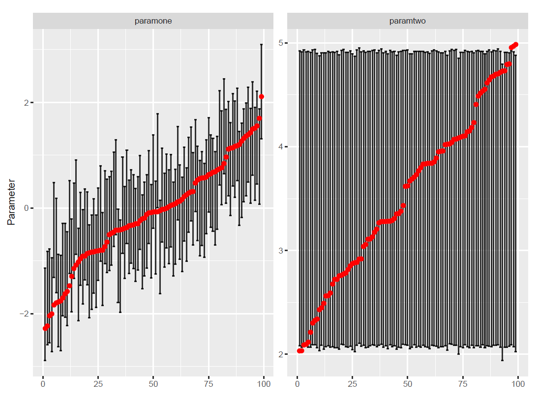
Now we can estimate the model using the real data, which here we pretend to be ssone=1.37 and sstwo=1.11.
estimates<-
  freelunch::fit_gam(training_runs = reference_table,
                     target_runs = c(1.37,1.11),
                      parameter_colnames = c("paramone","paramtwo"),
                                summary_statistics_colnames = c("ssone","sstwo"))
Which estimates paramone somewhere between -0.3 and 1.49 while paramtwo across its whole range:
estimates$predictions
#> # A tibble: 1 x 2
#>   paramone paramtwo
#>      <dbl>    <dbl>
#> 1    0.605     3.49

estimates$lows
#> # A tibble: 1 x 2
#>   paramone paramtwo
#>      <dbl>    <dbl>
#> 1   -0.279     2.08

estimates$highs
#> # A tibble: 1 x 2
#>   paramone paramtwo
#>      <dbl>    <dbl>
#> 1     1.50     4.91
An ill-posed example
The classic example of under-identified model: two people with weights weight1 and weight2 stand together on a scale and we read their combined weight total.
Reading only total we are asked to get the two individual weights. We observe the total weight of 5,000 pairs of people. There is already an example of this in the package so we just load it here:
data("scale_experiment")
glimpse(scale_experiment)
#> Rows: 5,000
#> Columns: 3
#> $ total   <dbl> 259.8286, 244.7187, 213.4538, 248.0799, 213.7402, 278.4608,...
#> $ weight1 <dbl> 135.94215, 126.21180, 121.82348, 123.92908, 125.67809, 129....
#> $ weight2 <dbl> 123.24073, 118.69401, 92.68997, 123.20384, 87.20287, 149.87...
We can try to solve this problem with rejection ABC and random forests. We first perform a standard set of cross-validations:
abc.cv<-cross_validate_rejection_abc(total_data = scale_experiment,
                                     parameter_colnames = c("weight1","weight2"),
                                     summary_statistics_colnames = c("total"))

rf.cv<-cross_validate_random_forest(total_data = scale_experiment,
                                    parameter_colnames = c("weight1","weight2"),
                                    summary_statistics_colnames = c("total"))
We then discover that rejection ABC performs better than random forests for both parameters. This makes sense since the main advantage of random forests (weighing multiple conflicting summary statistics) is null here.
##
abc.cv$performance
#>   weight1   weight2
#> 0.2809824 0.2913560
rf.cv$performance
#>   weight1   weight2
#> 0.1734766 0.1845600
Now, while it is nice to know the general performance, a bit more analysis will provide further insights. For example here the performance of the rejection ABC is not consistent across the parameter space. The individual weights are easier to guess when both people are either very light or very heavy; the estimation will also work if both people on the scale are about of the same size since rejection ABC tends to default to averaging weights when in doubt. We can see this graphically plotting the average RMSE for a grid of parameters:
freelunch::plot_grid_rmse(abc.cv,parameter1="weight1",parameter2="weight2",
               intervals_first_parameter = 15,intervals_second_parameter = 15)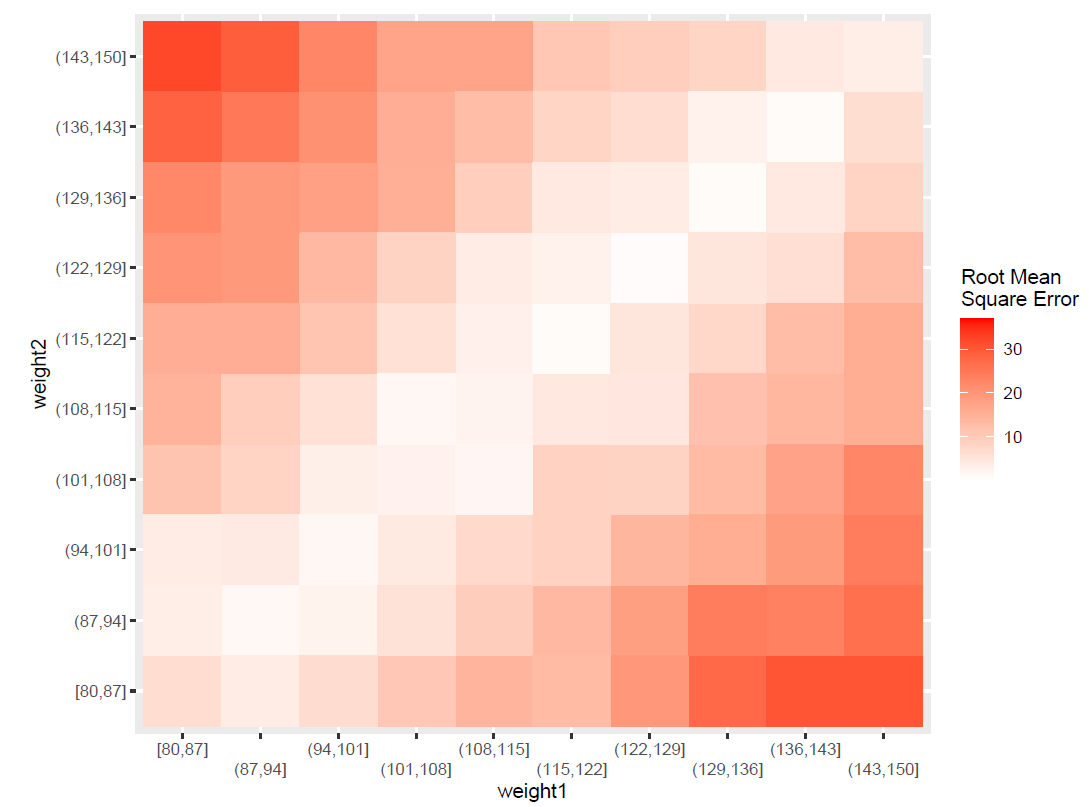
which is useful because it tells us that the method is very poor at estimating individual weights when one person is heavy and the other is thin.
Eventually if the applied work tells us that the “real life” observation we are trying to estimate has total=200, we can estimate with abc as follows:
abc.estimate<-fit_rejection_abc(training_runs = scale_experiment,
                                target_runs = c(200),
                                parameter_colnames = c("weight1","weight2"),
                                summary_statistics_colnames = c("total"))

abc.estimate$predictions
#>   weight1  weight2
#> 1 101.197 99.27007

abc.estimate$lows
#>    weight1  weight2
#> 1 81.04695 80.85538

abc.estimate$highs
#>    weight1  weight2
#> 1 121.9863 121.0303
Which guesses a weight of approximately 100 for both individuals, with a confidence interval between approximately 80 and 120.
References
ANDERSON, E. (1935). The Irises of the Gaspe Peninsula. Bulletin of the American Iris Society, 59, 2–5.
AXTELL, R. (1999). The emergence of firms in a population of agents: Local increasing returns to scale, unstable Nash equilibria, and power law size distributions. The Brookings Institution. Available at: https://www.brookings.edu/research/the-emergence-of-firms-in-a-population-of-agentslocal-increasing-returns-unstable-nash-equilibria-and-power-law-size-distributions/.
AXTELL, R. L., Epstein, J. M., Dean, J. S., Gumerman, G. J., Swedlund, A. C., Harburger, J., Chakravarty, S., Hammond, R., Parker, J., & Parker, M. (2002). Population growth and collapse in a multiagent model of the Kayenta Anasazi in Long House Valley. Proceedings of the National Academy of Sciences, 99(3), 7275–7279.
BEAUMONT, M. A., Zhang, W., & Balding, D. J. (2002). Approximate Bayesian computation in population genetics. Genetics, 162(4), 2025–2035.
BIANCHI, F., Grimaldo, F., Bravo, G., & Squazzoni, F. (2018). The peer review game: An agent-based model of scientists facing resource constraints and institutional pressures. Scientometrics, 116(3), 1401–1420.
BLUM, M. G. B., & Francois, O. (2010). Non-linear regression models for approximate Bayesian computation. Statistics and Computing, 20(1), 63–73.
BLUM, M. G. B., Nunes, M. A., Prangle, D., & Sisson, S. A. (2013). A comparative review of dimension reduction methods in approximate Bayesian computation. Statistical Science, 28(2), 189–208.
BORIA, E. S. (2020). Investing in the future by encouraging energy retrofit decisions. PhD thesis, University of Illinois at Chicago.
BREARCLIFFE, D. (2020). Non-Pharmaceutical herd immunity using homemade masks. International Conference on Social Computing, Behavioral-Cultural Modeling & Prediction and Behavior Representation in Modeling and Simulation.
BREIMAN, L. (2001). Random forests. Machine Learning, 45(1), 5–32.
BROEKE, G. ten, Voorn, G. van, & Ligtenberg, A. (2016). Which sensitivity analysis method should I use for my agent-based model? Journal of Artificial Societies and Social Simulation, 19(1), 5: https://jasss.soc.surrey.ac.uk/19/1/5.html.
CALVEZ, B., & Hutzler, G. (2006). Automatic tuning of agent-based models using genetic algorithms. In J. S. Sichman & L. Antunes (Eds.), Multi-Agent-Based simulation VI (pp. 41–57). Springer.
CANOVA, F., & Sala, L. (2009). Back to square one: Identification issues in DSGE models. Journal of Monetary Economics, 56(4), 431–449.
CARRELLA, E., Bailey, R. M., & Madsen, J. K. (2018). Indirect inference through prediction.
CARRELLA, E., Bailey, R. M., & Madsen, J. K. (2020). Calibrating Agent-Based models with linear regressions. Journal of Artificial Societies and Social Simulation, 23(1), 7: https://jasss.soc.surrey.ac.uk/23/1/7.html.
CLARK, J., & Crabtree, S. (2015). Examining social adaptations in a volatile landscape in northern Mongolia via the agent-based model Ger Grouper. Land, 4(1), 157–181.
CORNUET, J. M., Santos, F., Beaumont, M. A., Robert, C. P., Marin, J. M., Balding, D. J., Guillemaud, T., & Estoup, A. (2008). Inferring population history with DIY ABC: A user-friendly approach to approximate Bayesian computation. Bioinformatics, 24(23), 2713–2719.
CRANMER, K., Brehmer, J., & Louppe, G. (2020). The frontier of simulation-based inference. Proceedings of the National Academy of Sciences of the United States of America, 117(48), 30055–30062.
CREEL, M. (2017). Neural nets for indirect inference. Econometrics and Statistics, 2, 36–49.
CSILLÉRY, K., Francois, O., & Blum, M. G. B. (2012). Abc: An R package for approximate Bayesian computation (ABC). Methods in Ecology and Evolution, 3(3), 475–479.
DAVISON, A. C., & Hinkley, D. V. (1997). Bootstrap methods and their application. Cambridge University Press.
DELLI Gatti, D., Desiderio, S., Gaffeo, E., Cirillo, P., & Gallegati, M. (2011). Macroeconomics from the Bottom-Up. Springer.
DUGGER, A. (2020). OfficeMoves: Personalities and performance in an interdependent environment v1.0.0.
EDMONDS, B., Le Page, C., Bithell, E., M. Chattoe-Brown, Grimm, V., Meyer, R., Montañola-Sales, C., Ormerod, P., Root, H., & Squazzoni, F. (2019). Different modelling purposes. Journal of Artificial Societies and Social Simulation, 22(3), 6: https://jasss.soc.surrey.ac.uk/22/3/6.html
EPSTEIN, J. M., & Axtell, R. (1996). Growing artificial societies: Social science from the bottom up. Brookings Institution Press.
EPSTEIN, J. M., Cummings, D. A. T., Chakravarty, S., Singha, R. M., & Burke, D. S. (2012). Toward a containment strategy for smallpox bioterror: An individual-based computational approach. Brookings Institution Press.
FAGIOLO, G., Guerini, M., Lamperti, F., Moneta, A., & Roventini, A. (2019). 'Validation of agent-based models in economics and finance.' In Beisbart C., Saam N (Eds.), Computer Simulation Validation. Simulation Foundations, Methods and Applications. Berlin Heidelberg, Springer Verlag: 763–787.
FASIOLO, M., & Wood, S. N. (2014). An introduction to synlik. Available at: https://cran.r-project.org/web/packages/synlik/vignettes/synlik.html.
FERNÁNDEZ-VILLAVERDE, J., Rubio Ramírez, J. F., & Schorfheide, F. (2016). 'Solution and estimation methods for DSGE models.' In J. B. Taylor & H. Uhlig (Eds.), Handbook of Macroeconomics. (pp. 527–724). North-Holland.
FLACHE, A., & Matos Fernandes, C. A. de. (2021). 'Agent-based computational models.' In G. Manzo (Ed.), Research Handbook on Analytical Sociology. Edward Elgar.
FRANCIS, A. R., Sisson, S. A., Jiang, H., Luciani, F., & Tanaka, M. M. (2009). The epidemiological fitness cost of drug resistance in Mycobacterium tuberculosis. Proceedings of the National Academy of Sciences, 106(34), 14711–14715.
FRIEGE, J., Holtz, G., & Chappin, E. J. L. (2016). Exploring homeowners’ insulation activity. Journal of Artificial Societies and Social Simulation, 19(1), 4: https://jasss.soc.surrey.ac.uk/19/1/4.html.
GELMAN, A., & Shalizi, C. R. (2013). Philosophy and the practice of Bayesian statistics. British Journal of Mathematical and Statistical Psychology, 66(1), 8–38.
GOURIEROUX, C., Monfort, A., & Renault, E. (1993). Indirect inference. Journal of Applied Econometrics, 8, 85–118.
GRAZZINI, J., & Richiardi, M. (2015). Estimation of ergodic agent-based models by simulated minimum distance. Journal of Economic Dynamics and Control, 51, 148–165.
GRAZZINI, J., Richiardi, M., & Tsionas, M. (2017). Bayesian estimation of agent-based models. Journal of Economic Dynamics and Control, 77, 26–47.
HARTIG, F., Calabrese, J. M., Reineking, B., Wiegand, T., & Huth, A. (2011). Statistical inference for stochastic simulation models - theory and application. Ecology Letters, 14(8), 816–827.
HASTIE, T., Tibshirani, R., & Friedman, J. (2009). The Elements of Statistical Learning. Berlin Heidelberg: Springer.
HEGSELMANN, R. (2017). Thomas C. Schelling and James M. Sakoda: The intellectual, technical, and social history of a model. Journal of Artificial Societies and Social Simulation, 20(3), 15: https://jasss.soc.surrey.ac.uk/20/3/15.html.
HOOTEN, M., Wikle, C., & Schwob, M. (2020). Statistical implementations of agent‐based demographic models. International Statistical Review, 88(2), 441–461.
IASIELLO, C., Crooks, A., & Wittman, S. (2020). 'The human resource management parameter experimentation tool.' In R. Thomson, H. Bisgin, C. Dancy, A. Hyder, & M. Hussain (Eds.), Social, Cultural, and Behavioral Modeling. (pp. 298–307). Berlin Heidelberg: Springer.
IZQUIERDO, L. R., IZQUIERDO, S. S., Galán, J. M., & Santos, J. I. (2008). Miller and Page’s standing ovation model.
JABOT, F. (2010). A stochastic dispersal-limited trait-based model of community dynamics. Journal of Theoretical Biology, 262(4), 650–661.
JABOT, F., Faure, T., & Dumoulin, N. (2013). EasyABC: Performing efficient approximate Bayesian computation sampling schemes using R. Methods in Ecology and Evolution, 4(7), 684–687.
JANSSEN, M. A. (2009). Understanding artificial Anasazi. Journal of Artificial Societies and Social Simulation, 12(4), 13: https://jasss.soc.surrey.ac.uk/12/4/13.html..
JANSSEN, M. A. (2020). Introduction to Agent-Based Modeling. https://books.apple.com/us/book/introduction-to-agent-based-modeling/id1493610378?ls=1.
JIANG, B., Wu, T. Y., Zheng, C., & Wong, W. H. (2017). Learning summary statistic for approximate Bayesian computation via deep neural network. Statistica Sinica, 27(4), 1595–1618.
KARABATSOS, G., & Leisen, F. (2017). An approximate likelihood perspective on ABC methods. Statistics Surveys, 12, 66–104.
KLIMA, G., Podemski, K., & Retkiewicz-Wijtiwiak, K. (2018). gEcon: General equilibrium economic modelling language and solution framework. Available at: https://gecon.r-forge.r-project.org/files/gEconusers-guide.pdf.
KUHN, M. (2008). Building predictive models in R using the caret package. Journal of Statistical Software, 28(5), 1–26.
KURAHASHI, S. (2016). A health policy simulation model of Ebola haemorrhagic fever and Zika fever. In G. Jezic, Y. H. J. Chen-Burger, R. J. Howlett, & L. C. Jain (Eds.), Agent and Multi-Agent Systems: Technology and Applications. (pp. 319–329). Berlin Heidelberg: Springer.
LEBARON, B. (2001). Stochastic volatility as a simple generator of apparent financial power laws and long memory. Quantitative Finance, 1(6), 621–631.
LEE, J. S., Filatova, T., Ligmann-Zielinska, A., Hassani-Mahmooei, B., Stonedahl, F., Lorscheid, I., Voinov, A., Polhill, G., Sun, Z., & Parker, D. C. (2015). The complexities of agent-based modeling output analysis. Journal of Artificial Societies and Social Simulation, 18(4), 4: https://jasss.soc.surrey.ac.uk/18/4/4.html.
LEWBEL, A. (2019). The identification zoo: Meanings of identification in econometrics. Journal of Economic Literature, 57(4), 835–903.
LIGMANN-ZIELINSKA, A., Siebers, P. O., Magliocca, N., Parker, D. C., Grimm, V., Du, J., Cenek, M., Radchuk, V., Arbab, N. N., Li, S., Berger, U., Paudel, R., Robinson, D. T., Jankowski, P., An, L., & Ye, X. (2020). ’One size does not fit all’: A roadmap of purpose-driven mixed-method pathways for sensitivity analysis of agent-based models. Journal of Artificial Societies and Social Simulation, 23(1), 6: https://jasss.soc.surrey.ac.uk/23/1/6.html.
LINDKVIST, E. (2020). FishMob: Interactions between fisher mobility and spatial resource heterogeneity. CoMSES Computational Model Library. Available at: https://doi.org/10.25937/k7fx-cj36.
MAGLIOCCA, N., McConnell, V., & Walls, M. (2018). Integrating global sensitivity approaches to deconstruct spatial and temporal sensitivities of complex spatial agent-based models. Journal of Artificial Societies and Social Simulation, 21(1), 12: https://jasss.soc.surrey.ac.uk/21/1/12.html.
MEINSHAUSEN, N. (2006). Quantile regression forests. Journal of Machine Learning Research, 7, 983–999.
MEINSHAUSEN, N. (2017). QuantregForest: Quantile regression forests. Available at: https://cran.r-project.org/package=quantregForest.
MILLER, J. H., & Page, S. E. (2004). The standing ovation problem. Complexity, 9(5), 8–16.
MILLER, J. H., & Page, S. E. (2009). Complex adaptive systems: An introduction to computational models of social life. Princeton, NJ: Princeton University Press.
MONTI, C., De Francisci Morales, G., & Bonchi, F. (2020). Learning opinion dynamics from social traces. Proceedings of the ACM SIGKDD International Conference on Knowledge Discovery and Data Mining, 764-773.
NUNES, M. A., & Prangle, D. (2015). abctools: An R package for tuning approximate Bayesian computation analyses. The R Journal, 7(2), 189–205.
PIETZSCH, B., Fiedler, S., Mertens, K. G., Richter, M., Scherer, C., Widyastuti, K., Wimmler, M. C., Zakharova, L., & Berger, U. (2020). Metamodels for evaluating, calibrating and applying agent-Based models: A review. Journal of Artificial Societies and Social Simulation, 23(2), 9: https://jasss.soc.surrey.ac.uk/23/2/9.html.
PLATAS-LÓPEZ, A., Guerra-Hernández, A., Cecconi, F., Paolucci, M., & Grimaldo, F. (2019). Micro-foundations of macroeconomic dynamics: The agent-based BAM model. Frontiers in Artificial Intelligence and Applications, 319(2), 319–328.
PLATT, D. (2020). A comparison of economic agent-based model calibration methods. Journal of Economic Dynamics and Control, 319, 103859.
POILE, C., & Safayeni, F. (2016). Using computational modeling for building theory: A double edged sword. Journal of Artificial Societies and Social Simulation, 19(3), 8: https://jasss.soc.surrey.ac.uk/19/3/8.html.
PRANGLE, D. (2017). gk: An R package for the g-and-k and generalised g-and-h distributions. Available at: http://arxiv.org/abs/1706.06889.
PRANGLE, D., Fearnhead, P., Cox, M. P., Biggs, P. J., & French, N. P. (2014). Semi-automatic selection of summary statistics for ABC model choice. Statistical Applications in Genetics and Molecular Biology, 13(1), 67–82.
PRITCHARD, J. K., Seielstad, M. T., Perez-Lezaun, A., & Feldman, M. W. (1999). Population growth of human Y chromosomes: A study of y chromosome microsatellites. Molecular Biology and Evolution, 16(12), 1791–1798.
RAILSBACK, S. F., & Grimm, V. (2011). Agent-Based and Individual-Based Modeling: A practical introduction. Princeton, NJ: Princeton University Press.
RAYNAL, L., Marin, J. M., Pudlo, P., Ribatet, M., Robert, C. P., & Estoup, A. (2019). ABC random forests for Bayesian parameter inference. Molecular Biology and Evolution, 35(10), 1720–1728.
ROLLINS, N. D., Barton, C. M., Bergin, S., & Janssen, M. A. (2014). A computational model library for publishing model documentation and code. Environmental Modelling & Software, 61, 59–64.
RUBIO, F. J., & Johansen, A. M. (2013). A simple approach to maximum intractable likelihood estimation. Electronic Journal of Statistics, 7(1), 1632–1654.
SAKODA, J. M. (1971). The checkerboard model of social interaction. The Journal of Mathematical Sociology, 1(1), 119–132.
SALLE, I., & Yıldızoğlu, M. (2014). Efficient sampling and meta-modeling for computational economic models. Computational Economics, 44(4), 507–536.
SCHELLING, T. C. (1971). Dynamic models of segregation. The Journal of Mathematical Sociology, 1(2), 143–186.
SECCHI, D., & Gullekson, N. L. (2016). Individual and organizational conditions for the emergence and evolution of bandwagons. Computational and Mathematical Organization Theory, 22(1), 88–133.
SISSON, S. A., Fan, Y., & Tanaka, M. M. (2016). Sequential Monte Carlo without likelihoods. Proceedings of the National Academy of Sciences of the United States of America, 104(6), 1760–1765.
SMITH, A. A. (2008). Indirect inference. In M. Vernengo, E. P. Caldentey, & B. J. Rosser Jr (Eds.), The New Palgrave Dictionary of Economics (pp. 1–6). Palgrave Macmillan UK.
SNOEK, J., Larochelle, H., & Adams, R. P. (2012). Practical Bayesian optimization of machine learning algorithms. Proceedings of the 25th International Conference on Neural Information Processing Systems.
SOTNIK, G., Davidovsky, M., & Fedorenko, E. (2019). CEMMA: An interdisciplinary game for spatiotemporal common-pool resource management analysis.
STOW, C. A., Jolliff, J., McGillicuddy, D. J., Doney, S. C., Allen, J. I., Friedrichs, M. A. M., Rose, K. A., & Wallhead, P. (2009). Skill assessment for coupled biological/physical models of marine systems. Journal of Marine Systems, 76(1–2), 4–15.
THIELE, J. C., Kurth, W., & Grimm, V. (2014). Facilitating parameter estimation and sensitivity analysis of agent-based models: A cookbook using NetLogo and R. Journal of Artificial Societies and Social Simulation, 17(3), 11: https://jasss.soc.surrey.ac.uk/17/3/11.html.
TONI, T., Welch, D., Strelkowa, N., Ipsen, A., & Stumpf, M. P. H. (2009). Approximate Bayesian computation scheme for parameter inference and model selection in dynamical systems. Journal of the Royal Society Interface, 6(31), 187–202.
VAART, E. van der, Beaumont, M. A., Johnston, A. S. A., & Sibly, R. M. (2015). Calibration and evaluation of individual-based models using Approximate Bayesian Computation. Ecological Modelling, 312, 182–190.
VOORN, G. van, Hengeveld, G., & Verhagen, J. (2020). An agent based model representation to assess resilience and efficiency of food supply chains. PLoS ONE, 15(11), e0242323.
WAGER, S., Hastie, T., & Efron, B. (2014). Confidence intervals for random forests: The jackknife and the infinitesimal jackknife. Journal of Machine Learning Research, 15(2014), 1625–1651.
WILENSKY, U., & Reisman, K. (2006). Thinking like a wolf, a sheep, or a firefly: Learning biology through constructing and testing computational theories - An embodied modeling approach. Cognition and Instruction, 24(2), 171–209.
WILKINSON, R. (2013). Approximate Bayesian Computation (ABC). Available at: http://media.nips.cc/Conferences/2013/Video/Tutorial2B.pdf.
WILL, M., Groeneveld, J., Frank, K., & Müller, B. (2021). Informal risk-sharing between smallholders may be threatened by formal insurance: Lessons from a stylized agent-based model. PLoS ONE, 16(3), e0248757.
WILLIAMS, T. G., Guikema, S. D., Brown, D. G., & Agrawal, A. (2020). Assessing model equifinality for robust policy analysis in complex socio-environmental systems. Environmental Modelling & Software, 134, 104831.
WOLPERT, D. H. (2011). The supervised learning No-Free-Lunch theorems. Santa Fe Institute, New Mexico.
WOLPERT, D. H., & Macready, W. G. (1995). 'No free lunch theorems for search.' In R. Roy, M. Köppen, S. Ovaska, T. Furuhashi & F. Hoffmann (Eds.), Soft Computing and Industry, (pp. 25–42). Berlin Heidelberg: Springer.
WOOD, S. N. (2004). Stable and efficient multiple smoothing parameter estimation for generalized additive models. Journal of the American Statistical Association, 99(467), 673–686.
WOOD, S. N. (2010). Statistical inference for noisy nonlinear ecological dynamic systems. Nature, 466(7310), 1102–1104.
WOOD, S. N. (2017). Generalized additive models: An introduction with R. New York, NY: Chapman and Hall/CRC.
WOOD, S. N., & Augustin, N. H. (2002). GAMs with integrated model selection using penalized regression splines and applications to environmental modelling. Ecological Modelling, 157(2–3), 157–177.
WRIGHT, M. N., & Ziegler, A. (2017). ranger: A fast implementation of random forests for high dimensional data in C++ and R. Journal of Statistical Software, 77(1).
ZHAO, L. (2011). A model of limit-Order book dynamics and a consistent estimation procedure. Ann Arbor, MI: Umi Dissertation Publishing.