
Introduction
We want to tune the parameters of a simulation model to match data. When the likelihood is intractable and the data high-dimensional, the common approach is the simulated minimum distance (Grazzini & Richiardi 2015). This involves summarising real and simulated data into a set of summary statistics and then tuning the model parameters to minimize their distance. We show here the advantages of replacing this minimization with a regression.
Minimization involves three tasks. First, choose the summary statistics. Second, weight their distance. Third, perform the numerical minimization keeping in mind that simulation may be computationally expensive. Regressions bypass all three and estimate parameters directly (Sheehan & Song 2016; Creel 2017; Raynal et al. 2019; Radev et al. 2019). The current literature focuses on complex non-parametric regressions. Here we show that a simpler linear regularized regression will do.
First, run the model “many” times and observe which model parameters generate what kind of summary statistics. Then, regress the parameters as the dependent variable against all the simulated summary statistics. Finally, input the real summary statistics in the regression to obtain the tuned parameters. Model selection can be similarly achieved by training a classifier instead.
We summarize the agent-based estimation in general and regression methods in particular in Section 2. We describe how to parametrize models in Section 3. We then provide five examples: a statistical line fit in Section 4.1-4.14, an individual based biological model in Section 4.20-4.29, a non-linear differential equation in Section 4.30-4.35 and a fishery agent-based model in Section 4.36-4.54. We conclude by pointing out weaknesses in Section 5.
Literature Review
The approach of condensing data and simulations into a set of summary statistics in order to match them is covered in detail in two review papers: Hartig et al. (2011) in ecology and Grazzini & Richiardi (2015) in economics. They differ only in their definition of summary statistics: Hartig et al. (2011) defines it as any kind of observation available in both model and reality while Grazzini & Richiardi (2015), with its focus on consistency, allows only for statistical moments or auxiliary parameters from ergodic simulations.
Grazzini & Richiardi (2015) also introduces the catch-all term “simulated minimum distance” for a set of related estimation techniques, including indirect inference (Gourieroux, Monfort and Renault 1993) and the simulated method of moments (McFadden 1989). Smith (1993) first introduced indirect inference to fit a 6-parameter real business cycle macroeconomic model. In agent-based models, indirect inference was first advocated in Richiardi et al. (2006), see also Shalizi (2017), and first implemented in Zhao (2010) (who also proved mild conditions for consistency).
Common to all is the need to accomplish three tasks: selecting the summary statistics, defining the distance function and choosing how to minimize it.
Defining the distance function may at first appear the simplest of these tasks. It is standard to use the Euclidean distance between summary statistics weighed by the inverse of their variance or covariance matrix. However, while asymptotically efficient, this was shown to underperform in Smith (1993) and Altonji & Segal (1996). The distance function itself is a compromise, since in all but trivial problems we face a multi-objective optimization (see review by Marler & Arora 2004) where we should minimize the distance to each summary statistic independently. In theory, we could solve this by searching for an optimal Pareto front (see Badham et al. 2017, for an example of dominance analysis applied to agent-based models). In practice, however, even a small number of summary statistics make this approach unintelligible. Better then to focus on a single imperfect distance function (a weighted global criterion, in multi-objective optimization terms) where there is at least the hope of effective minimization. A practical solution that may nonetheless obscure tradeoffs between summary statistic distances.
We can minimize distance function with off-the-shelf methods such as genetic algorithms (Calver & Hutzler 2006; Heppenstall et al. 2007; Lee et al. 2015) or simulated annealing (Le et al. 2016; Zhao 2010). More recently two Bayesian frameworks have been prominent: BACCO (Bayesian Analysis of Computer Code Output) and ABC (Approximate Bayesian Computation).
BACCO involves running the model multiple times for random parameter inputs, building a statistical meta-model (sometimes called emulator or surrogate) predicting distance as a function of parameters and then minimizing the meta-model as a short-cut to minimizing the real distance. Kennedy & O’Hagan (2001) introduced the method (see A. O’Hagan 2006, for a review). Ciampaglia (2013), Parry et al. (2013) and Salle & Yıldızoğlu (2014) are recent agent-based model examples.
A variant of this approach interleaves running simulations and training the meta-model to sample more promising areas and achieve better minima. The general framework is the “optimization by model fitting” (see chapter 9 of Luke 2013, for a review; see Michalski 2000, for an early example). Lamperti, Roventini and Sani (2018) provided an agent-based model application (using gradient trees as a meta-model). Bayesian optimization (see Shahriari et al. 2016, for a review) is the equivalent approach using Gaussian processes and Bailey et al. (2018) first applied it to agent-based models.
As in BACCO, ABC methods also start by sampling the parameter space at random but retain only simulations whose distance is below a pre-specified threshold in order to build a posterior distribution of acceptable parameters (see Beaumont 2010, for a review). Drovandi et al. (2011), Lagarrigues et al. (2015, Grazzini et al. (2017) and Zhang et al. (2017) applied the method to agent-based models. Zhang et al. (2017) noted that ABC matches the “pattern oriented modelling” framework of Grimm et al. (2005).
All these algorithms however require the user to select the summary statistics first. This is always an ad-hoc procedure. Beaumont (2010) described it as “rather arbitrary” and noted that its effects “[have] not been systematically studied” and Kukacka & Barunik (2017) considered this the hardest part of simulated minimum distance. The more summary statistics we use, the more informative the simulated distance is (see Bruins et al. 2018, which compared four auxiliary models of increasing complexity). However, the more summary statistics we use the harder the minimization (and the more important the weighting of individual distances) becomes.
Because of its rejection approach, ABC methods are particularly vulnerable to the “curse of dimensionality” with respect to the number of summary statistics. As a consequence, the ABC literature has developed many “dimension reduction” techniques (see Blum et al. 2013, for a review). Of particular interest here is the use of regressions. Regressions in the ABC literature take two forms: first as semi-automatic ABC (Prangle et al. 2014), where linear regressions (or neural networks as in Jiang et al. 2017) are used on part of the data to project the rest in a space where rejection ABC may be more effective (effectively reweighting summary statistics); second as “regression-adjustments” (Beaumont et al. 2002; Blum & Francois 2010; Nott et al. 2011) which substitute the pre-specified rejection threshold with a localized regression.
The natural evolution of this approach is to abandon ABC altogether and simply regress the model parameters (dependent variables) on the summary statistics (independent variables). Raynal et al. (2019) does this with quantile random forest regressions. A more complicated alternative is deep neural networks: Sheehan & Song (2016) and Radev et al. (2019) applied them to raw data itself (bypassing summary statistics altogether) but Creel (2017) showed that deep neural networks estimate parameters better when using manually selected summary statistics.
Missing is a justification for using such complicated regressions. Because the mapping between summary statistics and parameters is valuable on its own, we think there is an advantage in using regressions which are informative and easy to diagnose. We settled on elastic nets in this paper as they provide a good balance: their parameters can be interpreted as those of an ordinary least square but, through regularization, the method is more robust to misspecification, collinearity and automatically selects away uninformative summary statistics.
Model selection in agent-based models has received less attention but the estimation literature has followed a similar trajectory. One can use a regression adjustment ABC method (as in Lee, Drovandi and Pettitt 2015) or more directly by training a random forest classifier over the whole dataset (Pudlo et al. 2015). Again, however, we can show that directly running a simple regression is just as effective.
Method
Estimation
Take a simulation model depending on \(K\) parameters \(\theta = \left[ \theta_1,\theta_2,\dots,\theta_K \right]\) to output \(M\) simulated summary statistics \(S(\theta) = \left[ S_1(\theta), S_2(\theta),\dots,S_M(\theta) \right]\). That is, \(S(\theta) \) is a vector of summary statistics produced by the model when using $\theta$ as its parameters. Given real-world observed summary statistics \(S^*\) we want to find the parameter vector \(\theta^*\) that generated them. Our method proceeds as follows:
- Repeatedly run the model each time supplying it a random vector of parameters \(\hat \theta\)
- Collect for each simulation its output as summary statistics \(S(\hat \theta)\); \(S(\hat \theta)\) being summary statistics generated by feeding the model the parameter vector \(\hat \theta\).
- Run \(K\) separate regularized regressions, \(r_i\), one for each parameter. The parameter is the dependent variable and all the candidate summary statistics are independent variables:
- Input the “real” summary statistics S* in each regression to predict the “real” parameters \(\theta^*\)
| $$ \left\{\begin{matrix} \theta_1 = r_1(S_1,S_2,\dots,S_M)\\ \theta_2 = r_2(S_1,S_2,\dots,S_M)\\ \vdots \\ \theta_n = r_n(S_1,S_2,\dots,S_M) \end{matrix}\right.$$ |
In step 1 and 2, we use the model to generate a data-set: we repeatedly input random parameters \(\hat \theta\) and we collect the output \(\hat S_1,\dots,\hat S_M\) (see Table 1 for an example). In step 3, we take the data we generated and use it to train regressions (one for each model input) where we want to predict each model input \(\theta\) looking only at the model output \(S_1,\dots,S_M\). The regressions map observed outputs back to the inputs that generated them. Only in step 4 we use the real summary statistics (which we have ignored so far) to input into the regressions we built in step 3. The prediction the regressions make when we feed in the real summary statistics \(S^*\) are the estimated parameters \(\theta^*\).
| \(\hat \theta_1\) | \(\hat S_1\) | \(\hat S_2\) | \(\dots\) | \(\hat S_M\) |
| \(\vdots\) | \(\vdots\) | \(\vdots\) | \(\vdots\) | \(\vdots\) |
| \(\vdots\) | \(\vdots\) | \(\vdots\) | \(\vdots\) | \(\vdots\) |
The key implementation detail is to use regularized regressions and in particular elastic nets (Friedman et al. 2010). Elastic nets are regression whose functional form is the familiar linear regression:
| $$Y = X \beta + \epsilon$$ |
But where we estimate \(\beta\) by minimizing the sum of square residuals (as with ordinary least squares) plus two additional penalties: the LASSO penalty \(||\beta||\) and the ridge penalty \(||\beta||^2\):
| $$\hat \beta = \arg\min ||Y-X\beta||^2 + \lambda_1 ||\beta|| + \lambda_2 ||\beta||^2$$ |
Where \(\lambda_1,\lambda_2\) are hyper-parameters selected by cross-validation.
The penalties that elastic nets add to the sum of square residuals formula help to select and reweigh weak summary statistics. LASSO penalties automatically drop summary statistics that are uninformative. Ridge penalties lower the weight of summary statistics that are strongly correlated to each other. We can then start with a large number of summary statistics (anything we think may matter and that the model can reproduce) and let the regression select only the useful ones.
Compare this to simulated minimum distance. There, the mapping between model outputs \(S(\cdot)\) and inputs \(\theta\) is defined by the minimization of the distance function:
| $$\theta^* = \arg_{\theta}\min (S(\theta)-S^*) W (S(\theta)-S^*)$$ |
When using a simulated minimum distance approach, both the summary statistics \(S(\cdot)\) and their weights \(W\) need to be chosen before one can estimates \(\theta^*\) by explicitly minimizing the distance. In effect the \(\arg \min\) operator maps model output \(S(\cdot)\) to model input \(\theta\). Instead, in our approach, the regularized regression not only selects and weights summary statistics but, more importantly, also maps them back to model input. Hence, the regression bypasses (takes the place of) the usual minimization.
Model selection
We observe summary statistics \(S^*\) from the real world and we would like to know which candidate model \(\{m_1,\dots,m_n\}\) generated them. We can solve this problem by training a classifier against simulated data.
- Repeatedly run each model
- Collect for each simulation its generated summary statistics \(S(m_i)\)
- Build a classifier predicting the model by looking at summary statistics and train it on the data-set just produced:
- Insert ``real'' summary statistics \(S^*\) in the classifier to predict which model generated it
| $$i \sim g(S_1,S_2,\dots,S_M)$$ |
The classifier family \(g(\cdot)\) can also be non-linear and non-parametric. We used a multinomial regression with elastic net regularization (Friedman et al. 2010); its advantages is that the regularization selects summary statistics and the output is a classic logit formula that is easily interpretable.
Model selection cannot be done on the same data-set used for estimation. If the parameters of a model need to be estimated, the estimation must be performed on either a separate training data-set or the inner loop of a nested cross-validation (Hastie et al. 2009).
Examples
Fit lines
Regression-based methods ftt straight lines as well as ABC or simulated minimum distance
In this section we present a simplified one-dimensional parameterization problem and show that regression methods perform as well as ABC and simulated minimum distance.
We observe 10 summary statistics \(S^*=(S^*_0,\dots,S^*_9)\) generated by \(S_i=\theta i + \epsilon\) where \(\epsilon \sim \mathcal{N}(0,1)\) and \(\theta\) is the only model parameter. Assuming the model is correct, we want to estimate the \(\theta^*\) parameter that generated the observed \(S^*\). Because the model is a straight line, we could solve the estimation by least squares. Pretend however this model to be a computational black box where the connection between it and drawing straight lines is not apparent.
We run 1,000 simulations with \(\theta \sim U[0,2]\) (the range is arbitrary and could represent either a prior or the feasible interval), collecting each time the 10 simulated summary statistics \(\hat S(\theta_i)\). We then train a linear elastic net regression of the form:
| $$\theta = a + \sum_{i=0}^9 b_i \hat S_i$$ |
Table 2 shows the \(b\) coefficients of the regression. \(S_0\) contains no information about \(\theta\) (since it is generated as \(S_0 = \epsilon\)) and the regression correctly ignores it by dropping \(b_0\) (setting the coefficient to 0). The elastic net weights larger summary statistics more because the effect of \(\theta\) is larger there compared to the \(\epsilon\) noise.
| Term | Estimate |
| (Intercept) | 0.026 |
| b1 | 0.002 |
| b2 | 0.007 |
| b3 | 0.006 |
| b4 | 0.011 |
| b5 | 0.014 |
| b6 | 0.019 |
| b7 | 0.020 |
| b8 | 0.024 |
| b9 | 0.028 |
We test this regression by making it predict, out-of-sample, the \(\theta\) of 1000 more simulations looking only at their summary statistics. Figure 1 and Table 3 compare the estimation quality with those achieved by the standard rejection ABC and MCMC ABC (following Marjoram et al. 2003; Wegmann et al. 2009; both methods implemented in Jabot et al. 2015). All achieve similar error rates.
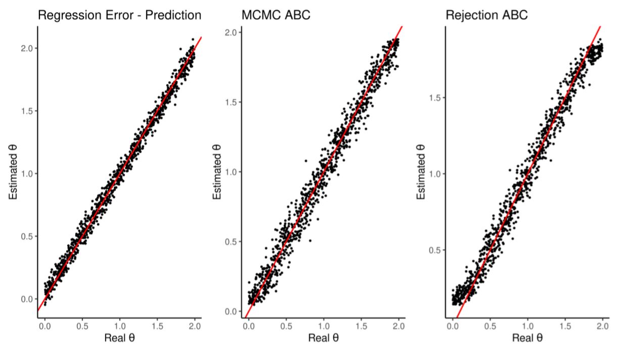
| Estimation | Average RMSE | Runtime | Runtime(scaled) |
| Regression Method | 0.053 | 0.0009 47 mins | 1.000 |
| Rejection ABC | 0.083 | 0.766 mins | 809.388 |
| MCMC ABC | 0.082 | 5.77 mins | 6090.665 |
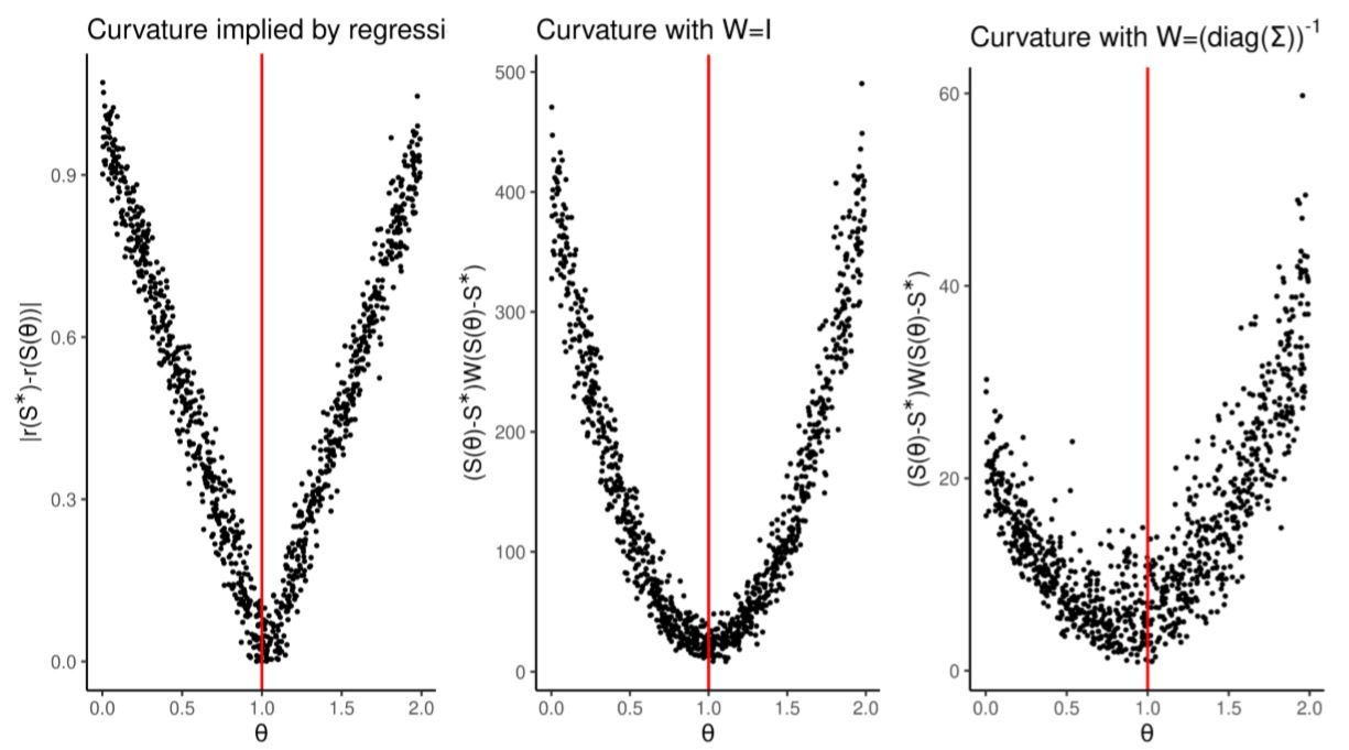
We can also compare the regression against the standard simulated minimum distance approach. Simulated minimum distance searches for the parameters that minimize:
| $$\theta^* = \arg_{\theta}\min (S(\theta)-S^*) W (S(\theta)-S^*) $$ |
The steeper its curvature, the easier it is to minimize numerically. In Figure 2 we compare the curvature defined by \(W=I\) and \(W= \left(\text{diag}(\Sigma)\right)^{-1}\) (where \(I\) is the identity matrix and \(\Sigma\) is the covariance matrix of summary statistics) against the curvature implied by our regression \(r\): \(|r(S^*)-r(S)|\) (that is, the distance between the estimation made given the real summary statistics, \(r(S^*)\), and the estimation made at other simulated summary statistics \(r(S)\)). This problem is simple enough that the all weight matrices produce smooth distance functions that are easy to numerically minimize.
We showed here that regression-based methods perform as well as ABC and simulated minimum distance in a simple one-dimensional problem.
Regression-based methods ftt broken lines better than ABC or simulated minimum distance
In this section we present another simplified one-dimensional parametrization but show that regression methods outperform both ABC and simulated minimum distance because of better selection of summary statistics.
We observe 10 summary statistics \(S=(S_0,\dots,S_9)\) but we assume they were generated by the ''broken line'' model:
| $$S_i=\left\{\begin{matrix} \epsilon & i < 5\\ \theta i + \epsilon & i\geq5 \end{matrix}\right.$$ |
As before we run the model 1000 times to train an elastic net of the form:
| $$\theta = a + \sum_{i=0}^9 b_i S_i$$ |
We run the model another 1000 times to test the regression ability to estimate their \(\theta\). As shown in Figure 3 and Table 5 the regression outperforms both ABC alternatives. This is due to the elastic net ability to prune unimportant summary statistics.
| Term | Estimate |
| (Intercept) | 0.037 |
| b5 | 0.018 |
| b6 | 0.021 |
| b7 | 0.023 |
| b8 | 0.029 |
| b9 | 0.027 |
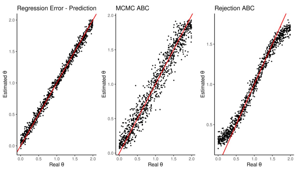
| Estimation | Average RMSE | Runtime | Runtime(scaled) |
| Regression Method | 0.058 | 0.0008255164 mins | 1.000 |
| Rejection ABC | 0.129 | 0.92158 mins | 1116.368 |
| MCMC ABC | 0.133 | 7.403095 mins | 8967.835 |
In simulated minimum distance methods, choosing the wrong \(W\) can compound the problem of poor summary statistics selection. As shown in Figure 4 the default choice \(W= \left(\text{diag}(\Sigma)\right)^{-1}\) spoils the curvature of the distance function by adding noise. This is because summary statistics \(S_0,\dots,S_4\), in spite of containing no useful information, are the values with the lowest variance and are therefore given larger weights in the simulated minimum distance framework.
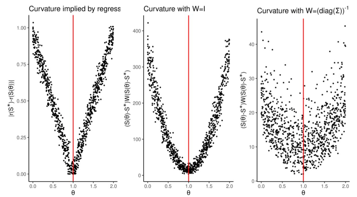
We showed here how, even in a simple one dimensional problem, the ability to prune uninformative summary statistics will result in better estimation (as shown by RMSE in Table 5).
Model selection through regression-based methods is informative and accurate
In this section, we train a classifier to choose which of the two models we described above (‘straight-’ and ‘broken-line’) generated the observed data. We show that the classifier makes fewer mistakes in identifying which model generated which data-set compared to always picking the model that minimizes prediction errors.
We observe 10 summary statistics \(S^*=(S^*_0,\dots,S^*_9)\) and we would like to know if they were generated by the “straight-line” model:
| $$S_i = \theta i + \epsilon $$ |
| $$S_i=\left\{\begin{matrix} \epsilon & i < 5\\ \theta i + \epsilon & i\geq5 \end{matrix}\right. $$ |
We run each model 1000 times and then train a logit classifier:
| $$\text{Pr}(\text{broken line model}) = \frac{1}{1 + \exp(-[a +\sum b_i S_i])} $$ |
Note that \(S_0\) and \(S_5,\dots,S_9\) are generated by the same rule in both models: both draw a straight line through those points. Their values will then not be useful for model selection. We should focus instead exclusively on \(S_1,\dots,S_4\) since that is the only area where one model draws a straight line and the other does not. The regularized regression discovers this, by dropping \(b_0\) and \(b_5,\dots,b_9\) as Table 6 shows.
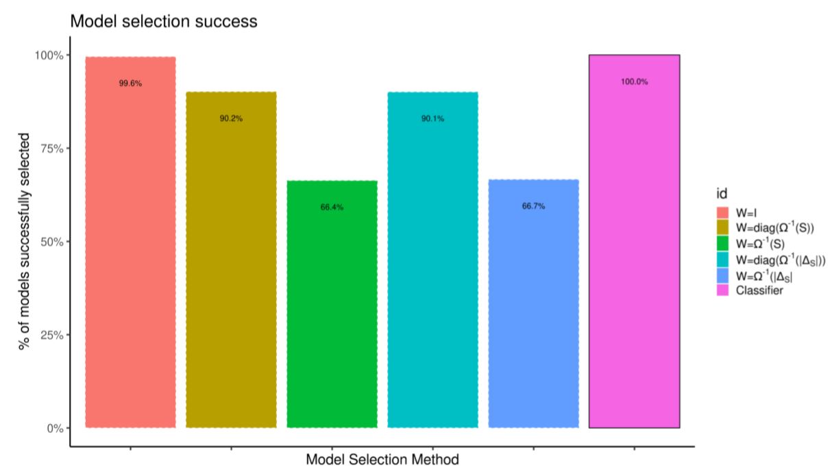
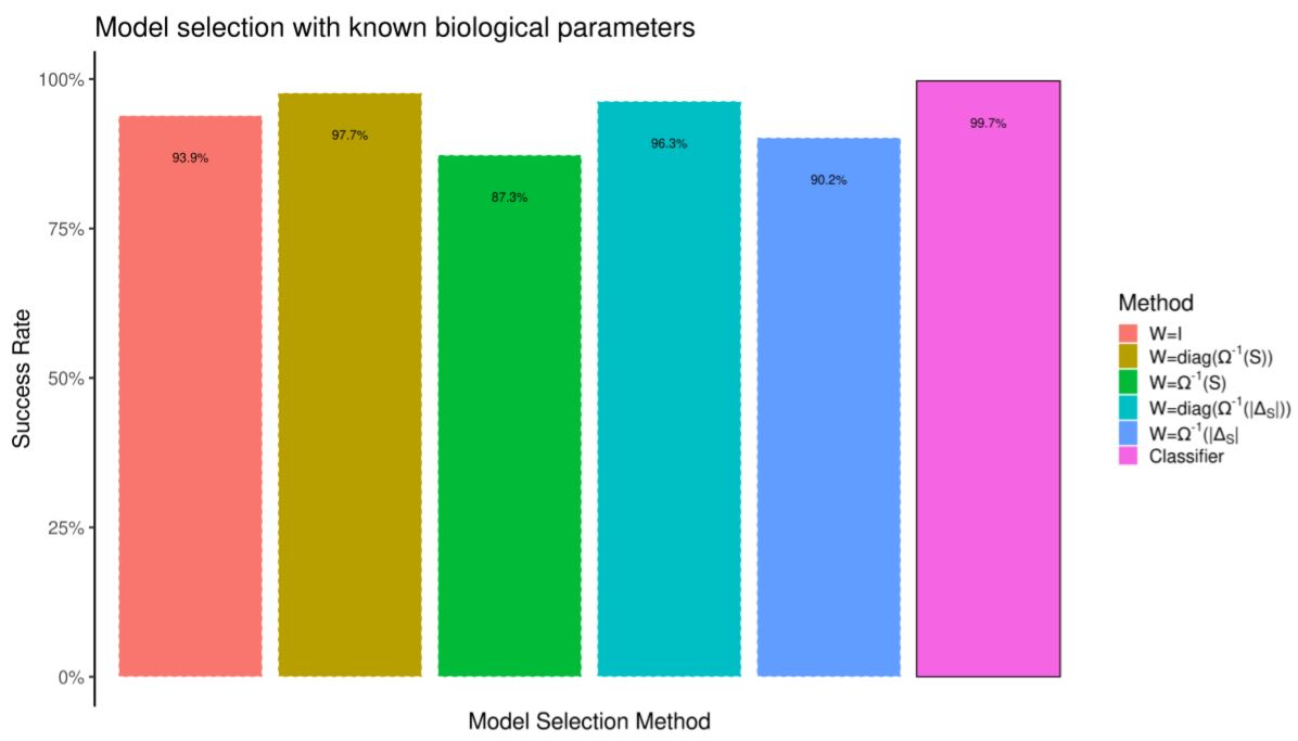
Figure 5 tabulates the success rate from 2000 out-of-sample simulations by the classifier and compares it with picking models by choosing the one that minimizes the distance between summary statistics. The problem is simple enough that choosing W = I achieves almost perfect success rate; using the more common variance-based weights does not.
| Term | Estimate |
| (Intercept) | -9.705 |
| b0 | 0.043 |
| b1 | 0.630 |
| b2 | 1.131 |
| b3 | 1.407 |
| b4 | 1.952 |
Fit ecological individual based model
In this section, we parametrize a simple agent-based model and prove two points. First, regularization is necessary because of the large number of summary statistics that agent based models generate. Second, directly regressing is more efficient than using regression-adjusted ABC, especially when the number of runs available is limited (a common problem for many agent-based models that are big and slow). To prove the second point we compare our results to those obtained by using the “semi-automatic” ABC method (Fearnhead & Prangle 2012; Prangle et al. 2014; implemented in Nunes & Prangle 2015) and neural network adjusted ABC (Blum 2010; implemented in Csillery et al. 2012).
We parametrize the bird population model from Thiele et al. (2014) and Railsback & Grimm (originally in 2012). This model is open source and Thiele et al. (2014) already estimated it using simulated annealing, genetic algorithms and ABC. All these approaches however failed to deal with the model under-identification since one of its two parameters could not be recovered. In this section we overcome this by using more summary statistics and weighting them correctly.
The bird population model depends on two parameters: scout.prob \(\in [0,.05]\), the probability of a non-alpha bird to explore a new territory, and survival.prob \(\in [.95,1]\), the monthly survival rate of each bird (Thiele et al. 2014, provides the ODD description and we attach a copy of the code in the supplementary materials). The original authors focused on 3 summary statistics: abundance (number of birds present at the end of each year), its standard deviation and vacancy (number of areas with no birds present). The model runs for 20 years and its summary statistics are the 20 years averages.
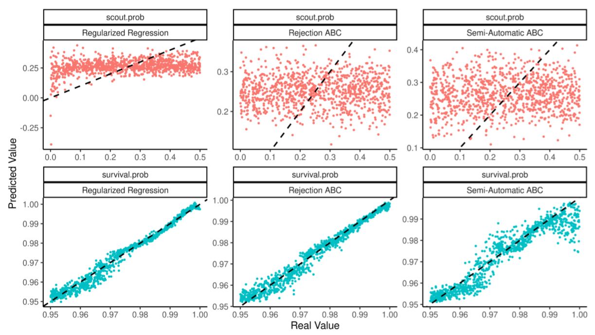
So structured, the calibration fails to identify the parameter scout.prob. We can show this by estimating the model (using RNetLogo Thiele et al. 2012; Thiele 2014) by rejection ABC (Beaumont, Zhang & Balding 2002; implemented in (Jabot et al. 2015), semi-automatic ABC (Fearnhead & Prangle 2012; implemented in Nunes & Prangle 2015) and regularized regressions.
Figure 6 compares real parameters and their out of sample estimates using a training set of 125 simulations. Table 7 judges the quality of the estimation through the predictivity coefficient (see Salle & Yıldızoğlu 2014; also known as modelling efficiency as in Stow et al. 2009) which measures the improvement of using an estimate \(\hat \theta\) to discover the real \(\theta^*\) as opposed to just using its average \(\bar \theta\):
| $$\text{Predictivity} = \frac{ \sum \left( \theta^*_i - \bar \theta \right)^2 - \sum \left( \theta^*_i - \hat \theta_i \right)^2 }{\sum \left( \theta^*_i - \bar \theta \right)^2} $$ |
A predictivity of 1 implies perfect estimation, 0 implies that averaging would have performed as well as the estimate. A predictivity below 0 that the parameter is misidentified.
| Algorithm | scout.prob | survival.prob |
| Regularized Regression | 0.046 | 0.979 |
| Rejection ABC | -0.065 | 0.974 |
| Semi-Automatic ABC | -0.100 | 0.886 |
scout.prob parameter is not.Under-identification is often an intrinsic part of the model. In this case, low scout.prob leads to population collapse and since all collapses look the same it is hard to find precisely which parameter value caused it. Under-identification may however matter if policy-making or predictions hinge on precise estimates of all parameters. One way to solve this problem is to use a larger set of summary statistics in the hope that they may contain more information.
As before, we collect the yearly time series of abundance and vacancy to which we add two yearly histograms: the distribution of average age in each group and the month in which groups explored. For each time series, we extract its trend, its average, its last value, its standard deviation, its range and the coefficients of fitting an AR(5) regression to it (for a total of 11 summary statistics). For each histogram, we extract four time series: its mean, its variance, its skewness and the total number of observations. Each of these time series is then split into summary statistics as above.
Using a regularized regression, we can use all these summary statistics (as well as their squares and their cross products) to recover the two original parameters. A similar attempt using semi-automatic ABC techniques (with default threshold rate of 10%) will not perform as well. This is due to two factors. First, by not using regularization semi-automatic ABC requires more simulations than summary statistics; for small training set then the semi-automatic ABC approach cannot even be applied while regularized regressions already provide good parameter estimates. Second, semi-automatic ABC splits the training data in two, feeding half of it to a linear regression and uses its weights to perform ABC on the other half. This exacerbates linear regression tendency to overfit by feeding it too little data. An alternative is to use a non-parametric technique with ABC such as the neural-network approach suggested in Blum (2010). However, the same problems of overfitting (too many explanatory variables fitting over too few simulation runs) mar this approach unless the size of the training set is large.
Table 8 and Figure 7 show how the scout.prob parameter is now identified and regularized regressions outperforms the alternatives. The table also shows that for small and medium sized training tests semi-automatic ABC performs not only worse than running a regularized regression, but worse than running a plain linear regression as well. Neural network ABC struggles by making rare but large prediction errors.
| Training Observations | Regularized Regression | Linear Regression | saABC | NN ABC |
| 125 | 0.467 | -0.488 | NA | -0.198 |
| 150 | 0.539 | -0.004 | NA | 0.076 |
| 250 | 0.610 | 0.408 | 0.169 | 0.275 |
| 500 | 0.676 | 0.542 | 0.447 | 0.222 |
| 1000 | 0.701 | 0.579 | 0.578 | 0.584 |
| 5000 | 0.765 | 0.607 | 0.645 | 0.820 |
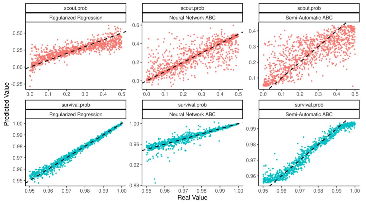
scout.prob parameter is estimated correctly by all three methods, but more precisely by the regularized regression (with neural-network making rare but large mistakes).Estimating a non-linear population model
When we can generate many training simulations to parametrize the model, the advantages of regularization are reduced and one may be better off using more complex non-parametric regressions. Even under these circumstances however, estimating parameters through regularized linear regressions is still viable as it achieves predictivity only slightly below neural network ABC (and still superior to semi-automatic ABC).
Gurney et al. (1980) introduced the following mathematical model to simulate blowfly population dynamic:
| $$\frac{dN}{dt} = P N(t-\tau)^{-\frac{N(t-\tau)}{N_0}} - \delta N(t)$$ |
Wood (2010) produced a stochastic and discretized version of this model which he then parametrized through synthetic likelihood. A C version of the model is implemented in the \synlik R package (Fasiolo & Wood 2014).
The model depends on 6 parameters: \(\delta \sim U[e^{-3},e^{-1}]\), \(P \sim U[e^{1},e^{3}]\), \(N_0 \sim U[e^{5},e^{7}]\), \(\sigma_p \sim U[e^{-2},e^{0}]\), \(\tau \sim U[e^{2.5},e^{2.9}]\) and \(\sigma_d \sim U[e^{-1.5},e^{0}]\). It generates 20 summary statistics: the mean \(N\), mean minus median, number of turning points observed, autocorrelation of \(N\) up until lag 11, and the polynomial autoregression of \(N\) on its lags as described in the methods summary of Wood (2010). Because the model is fast to run we generate 100,000 training and 1,000 testing simulations.
We estimate the parameters of the testing simulations by neural network ABC, semi-automatic ABC (degree 2, threshold of .1) as well as well as regularized linear regressions of both degree two (‘2D’, as usual) and three (‘3D’, which we can afford given the many observations).
Table 9 shows the predictivity associated with each method. Neural network ABC achieves the highest predictivity for 5 out of 6 parameters, even though the gains compared to a linearized regression are small. Only for \(\sigma_d\) (the hardest parameter to estimate) regularized linear regressions do better.
| Variable | Semi-Automatic ABC | Regularized Regression (2D) | Regularized Regression (3D) | Neural Network ABC |
| \(\delta\) | 0.745 | 0.913 | 0.935 | 0.944 |
| \(N_0\) | 0.741 | 0.910 | 0.927 | 0.934 |
| \(P\) | 0.566 | 0.717 | 0.780 | 0.807 |
| \(\tau\) | 0.600 | 0.802 | 0.843 | 0.863 |
| \(\sigma_d\) | 0.069 | 0.119 | 0.147 | 0.095 |
| \(\sigma_p\) | 0.270 | 0.322 | 0.413 | 0.473 |
Fit RBC
Fit against cross-correlation matrix
In this section, we parametrize a simple macro-economic model by looking at the time series it simulates. We show that we can use a large number of summary statistics efficiently and that we can diagnose estimation strengths and weaknesses the same way we diagnose regression outputs. We also show that regularized linear regressions outperform random forest regressions (a more complicated, non-parametric approach).
We observe 150 steps[1] of 5 quarterly time series: \(Y,r,I,C,L\). Assuming we know they come from a standard real business cycle (RBC) model (the default RBC implementation of the gEcon package in R, see Klima et al. 2018, see also Appendix A), we estimate the 6 parameters (\(\beta,\delta,\eta,\mu,\phi,\sigma\)) that generated them.
We summarize the time series observed with (a) the \(t=-5,\dots,+5\) cross-correlation vectors of \(Y\) against \(r,I,C,L\), (b) the lower-triangular covariance matrix of \(Y,r,I,C,L\), (c) the squares of all cross-correlations and covariances, (d) the pair-wise products between all cross-correlations and covariances. This totals to 2486 summary statistics: too many for most ABC approaches. This problem is however still solvable by regression. We train 6 separate regressions, one for each parameter, as follows:
| $$\left\{\begin{matrix} \beta &= \sum a_{\beta,i} S_i + \sum b_{\beta,i} S_{i}^2 + \sum c_{\beta,i,j} S_i S_j \\ \gamma &= \sum a_{\gamma,i} S_i + \sum b_{\gamma,i} S_{i}^2 + \sum c_{\gamma,i,j} S_i S_j \\ &\vdots \\ \sigma &= \sum a_{\sigma,i} S_i + \sum b_{\sigma,i} S_{i}^2 + \sum c_{\sigma,i,j} S_i S_j \\ \end{matrix}\right. $$ | (1) |
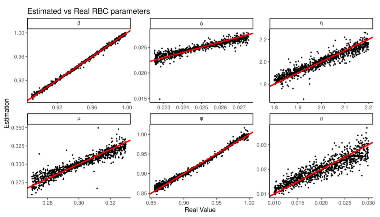
We train the regressions over 2000 RBC runs then produce 2000 more to test its estimation. Figure 8 and Table 10 shows that all the parameters are estimated correctly but \(\eta\) and \(\delta\) less precisely. Table 11 shows that regularized linear regression estimates all the parameters better than a random forest (Breiman 2001; using the R implementation from Liaw & Wiener 2002), suggesting that regularization and linearity have an advantage over non-parametrics when there are few training observations and many summary statistics.
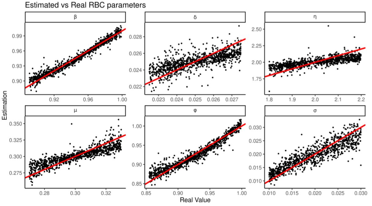
| Variable | Variable Bounds | Average Bias | Average RMSE | Predictivity |
| β | [0.891,0.999] | 0.0003070 | 0.0000360 | 0.963 |
| δ | [0.225,0.275] | -0.0000431 | 0.0000010 | 0.494 |
| η | [1.8,2.2] | -0.0009051 | 0.0062672 | 0.517 |
| μ | [0.27,0.33] | 0.0001420 | 0.0000761 | 0.746 |
| σ | [0.01,0.03] | -0.0000402 | 0.0000070 | 0.795 |
| φ | [0.855,0.999] | -0.0001569 | 0.0001229 | 0.925 |
| Variable | Regularized Regression | Random Forest |
| β | 0.963 | 0.953 |
| δ | 0.494 | 0.072 |
| η | 0.517 | -0.007 |
| μ | 0.746 | 0.034 |
| σ | 0.795 | 0.730 |
| φ | 0.925 | 0.882 |
We showed here that we can estimate the parameters of a simple RBC model by looking at their cross-correlations. However, this method is better served by looking at multiple auxiliary models as we show in the next section.
Fit against auxiliary fits
In this section, we parametrize the same simple macro-economic model by looking at the same time series it simulates but using a more diverse array of summary statistics. We show how that improves the estimation of the model.
Again, we observe 150 steps of 5 quarterly time series: \(Y,r,I,C,L\). Assuming we know they come from a standard RBC model, we want to estimate the 6 parameters (\(\beta,\delta,\eta,\mu,\phi,\sigma\)) that generated them.
| Variable | Regularized Regression | Random Forest |
| β | 0.997 | 0.986 |
| δ | 0.842 | 0.109 |
| η | 0.889 | 0.230 |
| μ | 0.880 | 0.030 |
| σ | 0.814 | 0.728 |
| φ | 0.988 | 0.920 |
| Variable | Regularized Regression | Random Forest |
| δ | 0.997 | 0.986 |
| η | 0.842 | 0.109 |
| μ | 0.889 | 0.230 |
| σ | 0.880 | 0.030 |
| φ | 0.814 | 0.728 |
| δ | 0.988 | 0.920 |
In this section we use a larger variety of summary statistics. We summarize output by (i) coefficients of regressing \(Y\) on \(Y_{t-1},I_{t},I_{t-1}\), (ii) coefficients of regressing \(Y\) on \(Y_{t-1},C_{t},C_{t-1}\), (iii) coefficients of regressing \(Y\) on \(Y_{t-1},r_{t},r_{t-1}\), (iv) coefficients of regressing \(Y\) on \(Y_{t-1},L_{t},L_{t-1}\), (v) coefficients of regressing \(Y\) on \(C,r\) (vi) coefficients of fitting AR(5) on \(Y\), (vii) the (lower triangular) covariance matrix of \(Y,I,C,r,L\). In total there are 48 summary statistics to which we add all their squares and cross-products.
Again we train 6 regressions over 2000 RBC observations and test their estimation against 2000 more. Figure 9 and Table 12 shows that all the parameters are estimated correctly and with higher predictivity coefficient. In particular \(\delta\) and \(\eta\) are better predicted than by looking at cross-correlations. Again, as shown in Table 13, regularized linear regressions outperform random forests.
Heuristic selection in the face of input uncertainty
In this section, we select between 10 variations of an agent-based model where some inputs and parameters are unknowable. By training a classifier, we are able to discover which summary statistics are robust to the unknown parameters and leverage this to outperform standard model selection by prediction error.
Assume all fishermen in the world can be described by one of 10 decision-making algorithms (heuristics). We observe 100 fishermen for five years and we want to identify which heuristic they are using. The heuristic selection is however complicated by not knowing basic biological facts about the environment the fishermen exploit. This is a common scenario in fisheries: we can monitor boats precisely through electronic logbooks and satellites but more than 80% of global catch comes from unmeasured fish stocks (Costello et al. 2012). Because heuristics are adaptive, the same heuristic will generate different summary statistics when facing different biological constraints. We show here that we can still identify heuristics even without knowing how many fish there are in the sea.
We can treat each heuristic as a separate model and train a classifier that looks at summary statistics to predict which heuristic generated them. The critical step is to train the classifier on example runs where the uncertain inputs (the unknown biological constraints) are randomized. This way the classifier automatically learns which summary statistics are robust to biological changes and look only at those when selecting the right heuristic.
We use POSEIDON (Bailey et al. 2018), a fishery agent-based model to simulate the fishery. We observe the fishery for five years and we collect 17 summary statistics: (i) aggregate five year averages on landings, effort (hours spent fishing), distance travelled from port, number of trips per year and average hours at sea per trip, (ii) a discretized (3 by 3 matrix) heatmap of geographical effort over the simulated ocean, (iii) the coefficients and R2 of a discrete choice model fitting area fished as a function of distance from port and habit (an integer describing how many times that particular fisher has visited that area before in the past 365 days ).
Within each simulation, all fishers use the same heuristic. There are 10 possible candidates, all described more in depth in a separate paper (Carrella et al. 2019):
- Random: each fisher each trip picks a random cell to trawl
- Gravitational Search: agents copy one another as if planets attracted by gravity where mass is equal to profits made in the previous trip (see Rashedi et al. 2009)
- s-greedy bandit: agents have a fixed 20% chance of exploring a new random area otherwise exploiting (fishing) the currently most profitable discovered location. Two parametrizations of this heuristic are available, depending on whether fishers discretize the map in a 3 by 3 matrix or a 9 by 9 one.
- “Perfect” agent: agents knows perfectly the profitability of each area \(\Pi(\cdot)\) and chooses to fish in area \(i\) by SOFTMAX:
| $$\text{Probability}(i) = \frac{e^{\Pi(i)}}{\sum_j e^{\Pi(j)}} $$ |
- Social Annealing: agents always return to the same location unless they are making less than fishery’s average profits (across the whole fishery), in which case they try a new area at random
- Explore-Exploit-Imitate: like \(\epsilon\)-greedy agents, they have a fixed probability of exploring. When not exploring each fisher checks the profits of two random “friends” and copies their location if either are doing better. Three parametrizations of this heuristics are possible: exploration rate at 80% or 20% with exploration range of 5 cells, or 20% exploration rate with exploration range of 20 cells.
- Nearest Neighbour: agents keep track of the profitability of all the areas they have visited through a nearest neighbour regression and always fish the peak area predicted by the regression.
All runs are simulations of the single-species “baseline” fishery described in the ESM of Bailey et al. (2018) (see also Appendix B). We run the model 10,000 times in total, 1000 times for each heuristic. We also randomize in each simulation three biological parameters: (i) carrying capacity of the each cell map, (ii) diffusion speed of fish, (iii) the Malthusian growth parameter of the stock.
We train a multi-logit classifier on the simulation outputs as shown in Sections 4.41-4.49:
| $$ \textit{Pr}(\textit{Heuristic }i) = \frac{e^{b_i' S}}{1+\sum_j e^{b_j' S}} $$ |
We build the testing data-set by running the model 10,000 more times. We compare the quality of model selection against selection by weighted prediction error. First, in Figure 10 the prediction error is computed by re-running simulations with the correct random biological parameters. In spite of having a knowledge advantage over the classifier, selection by prediction error performs worse. In Figure 11 we do not assume to know the random biological parameters. Prediction error (which now tries to minimize the distance between simulations which differ in both heuristics and biological parameters) performs much worse.
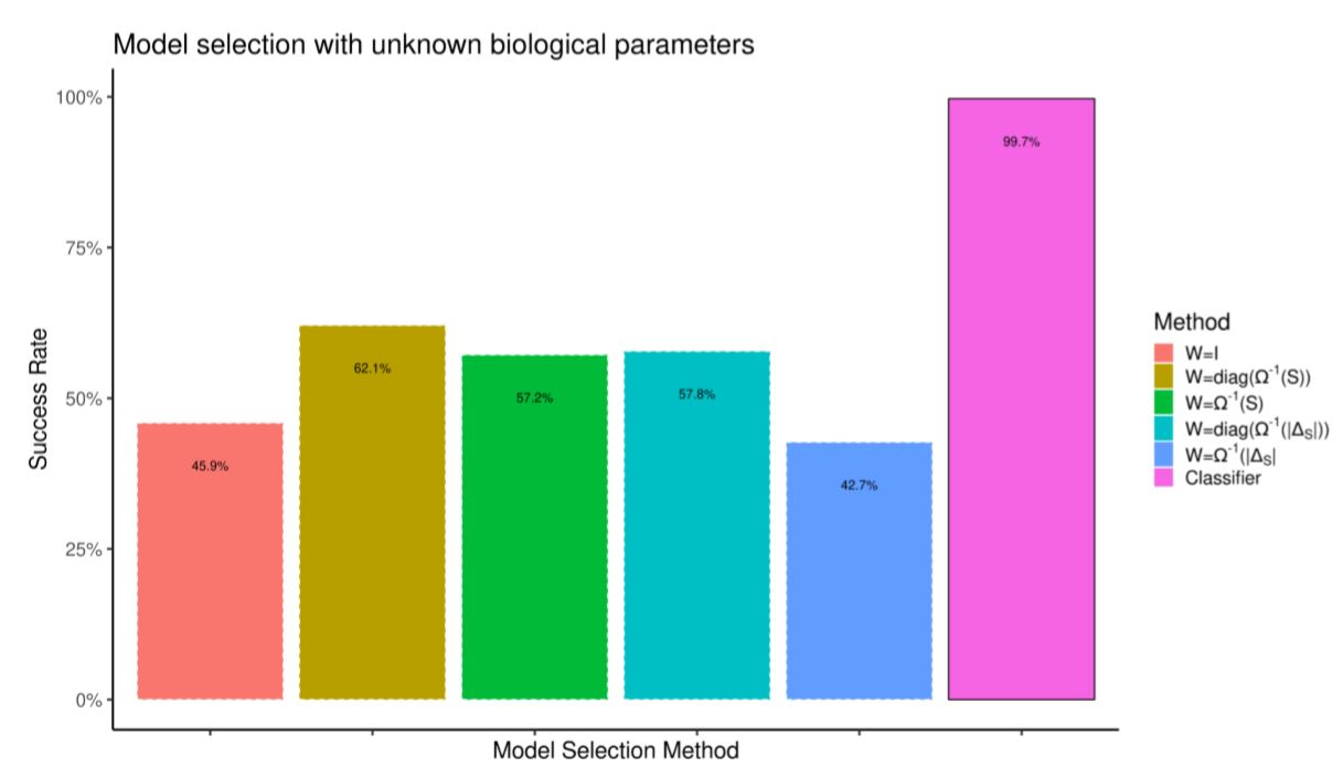
Model selection by prediction error is hard if we are not certain about all model inputs. However, it is trivial to train a classifier by feeding it observations from different parameter configurations such that only the summary statistics “robust” to such parameter noise are used for model selection.
Discussion
Advantages of a regression-based approach
Regressions are commonly-used and well-understood. We leverage that knowledge for parameter estimation. By looking at out-of-sample prediction we can immediately diagnose parameter identification problems: the lower the accuracy, the weaker the identification (compare this to diagnosis of numerical minimization outputs as in Canova & Sala 2009). Moreover, if the regression is linear, its coefficients show which summary statistic \(S_i\) inform which model parameter \(\theta_i\).
A secondary advantage of building a statistical model is the ease with which additional input uncertainty can be incorporated as shown in section 4.40. If we are uncertain about an input and cannot estimate it directly (because of lack of data or under-identification), it is straightforward to simulate for multiple values of the input, train a statistical model and then check whether it is possible to estimate reliably the other parameters. In a simulated minimum distance setting, we would have to commit to a specific guess of the uncertain input before running a minimization or minimize multiple times for each guess (without any assurance that the weighting matrix ought to be kept constant between guesses).
All the examples in this paper contained many more summary statistics than parameters. This seems to us as the most common parametrization problem facing an agent-based model. We showed that under these circumstances elastic net calibration correctly identifies informative summary statistics and avoid the overfitting that sometimes derails other algorithms. We also showed that this method degrades more gracefully than the alternatives when there are few training simulations, a problem that may emerge when parametrizing a slow model. However, if the number of summary statistics available is small or the model mispecified, there is probably not much that can be gained by regularization.
Weaknesses
This method has three limitations. First, users cannot weight summary statistics by importance. As a consequence, the method cannot be directed to replicate a specific summary statistic. Imagine a financial model of the housing market which we may judge primarily by its ability of matching real house prices. When estimating its parameters the regression may however ignore house prices entirely and focus on another seemingly minor summary statistic (say, total number of bathrooms). While that may be an interesting and useful way of parametrizing the model, it does not guarantee a good match with observed house prices. On the other hand, the emergence of seemingly minor summary statistics (bathrooms per house) as key variables to identify parameters of a model can be used as a signal that the model is mispecified. Nevertheless, in this case one option would be to transition to a weighted regression and weigh more the observations whose generated summary statistic \(S_i\) were close to the value of \(S_i^*\) we are primarily interested in replicating. As such, the model would be forced to include component deemed important, even if not the most efficient in terms of explanatory power. Comparing this fit with the unweighted one may also be instructive.
The second limitation is that each parameter is estimated separately. Be- cause each parameter is given a separate regression, this method may underestimate underlying connections (dependencies) between two or more parameters when such connections are not reflected in changes to summary statistics. This issue is mentioned in the ABC literature by Beaumont (2010) although it is also claimed that in practice it does not seem to be an issue. It may however be more appropriate to use a simultaneous system estimation routine (Henningsen & Hamann 2007) or a multi-task learning algorithm (Evgeniou & Pontil 2004).
The third limitation is that this method produces point estimates of parameters and not full confidence intervals. While prediction intervals could be used to estimate the range of valid parameters there is no frequentist analysis yet to produce valid confidence intervals (Kyung et al. 2010). One needs to use either a more complicated regression, such as the quantile random forests suggested by Raynal et al. (2019), or a simpler one where bootstrap prediction intervals are well defined (see Davison & Hinkley 1997).
Our method contains a fundamental inefficiency: we build a global statistical model to use only once when predicting for the real summary statistics \(S^*\). Given that the real summary statistics \(S^*\) are known in advance, a direct search ought to be more efficient. Our method makes up for this by solving multiple problems at once as it implicitly selects summary statistics and weights them while estimating the model parameters.
In machine learning, transduction substitutes regression when we are interested in a prediction for a known \(S^*\) only, without the need to build a global statistical model (see Chapter 10 of Cherkassky & Mulier 2007; Beaumont et al. 2002, weights simulations depending on the distance to known \(S^*\) in essentially the same approach). Switching to transduction would however remove the familiarity advantage of using regressions as well as the ease to test its predictive power with randomly generated summary statistics.
Conclusion
We presented here a general method to fit agent-based and simulation models. We performed indirect inference using prediction rather than minimization, and, by using regularized regressions, we avoided three major problems of estimation: selecting the most valuable of the summary statistics, defining the distance function, and achieving reliable numerical minimization. By substituting regression with classification, we can further extend this approach to model selection. This approach is relatively easy to understand and apply, and at its core uses statistical tools already familiar to social scientists. The method scales well with the complexity of the underlying problem, and as such may find broad application.
Acknowledgements
This research is funded in part by the Oxford Martin School, the David and Lucile Packard Foundation, the Gordon and Betty Moore Foundation, the Walton Family Foundation, and Ocean Conservancy.Notes
- This is the setup in the original indirect inference paper by Smith (1993) applied to a similar RBC model
Appendix
A: RBC Model
Consumer
| $$\begin{align}\max_{K^{\mathrm{s}}_{t}, C_{t}, L^{\mathrm{s}}_{t}, I_{t} } U_{t} = {\beta} {\mathrm{E}_{t}\left[U_{t+1}\right]} + \left(1 - \eta\right)^{-1} {\left({{C_{t}}^{\mu}} {\left(1 - L^{\mathrm{s}}_{t}\right)^{1 - \mu}}\right)^{1 - \eta}}\end{align}$$ | (2) |
| $$C_{t} + I_{t} = \pi_{t} + {K^{\mathrm{s}}_{t-1}} {r_{t}} + {L^{\mathrm{s}}_{t}} {W_{t}}$$ | (3) |
| $$K^{\mathrm{s}}_{t} = I_{t} + {K^{\mathrm{s}}_{t-1}} \left(1 - \delta\right)$$ | (4) |
Firm
| $$\max_{K^{\mathrm{d}}_{t}, L^{\mathrm{d}}_{t}, Y_{t} } \pi_{t} = Y_{t} - {L^{\mathrm{d}}_{t}} {W_{t}} - {r_{t}} {K^{\mathrm{d}}_{t}}$$ | (5) |
| $$Y_{t} = {Z_{t}} {{K^{\mathrm{d}}_{t}}^{\alpha}} {{L^{\mathrm{d}}_{t}}^{1 - \alpha}}$$ | (6) |
Equilibrium
| $$K^{\mathrm{d}}_{t} = K^{\mathrm{s}}_{t-1}$$ | (7) |
| $$L^{\mathrm{d}}_{t} = L^{\mathrm{s}}_{t}$$ | (8) |
| $$Z_{t} = e^{\epsilon^{\mathrm{Z}}_{t} + {\phi} {\log{Z_{t-1}}}} $$ | (9) |
| $$-0.36Y_\mathrm{ss} + {r_\mathrm{ss}} {K^{\mathrm{s}}_\mathrm{ss}} = 0 $$ | (10) |
B: Fishery parameters
| Parameter | Value | Meaning |
| Biology | Logistic | |
| K | \(\sim U[1000,10000]\) | max units of fish per cell |
| m | \(\sim U[0,0.003]\) | fish speed |
| r | \(\sim U[.3,.8]\) | Malthusian growth parameter |
| Fisher | Explore-Exploit-Imitate | |
| rest hours | 12 | rest at ports in hours |
| G | 0.2 | exploration rate |
| δ | \(\sim U[1,10]\) | exploration area size |
| fishers | number of fishers | |
| friendships | 2 | number of friends each fisher has |
| max days at sea | 5 | time after which boats must come home |
| Map | ||
| width | 50 | map size horizontally |
| height | 50 | map size vertically |
| port position | 40,25 | location of port |
| cell width | 10 | width (and height) of each cell map |
| Market | ||
| market price | 10 | $ per unit of fish sold |
| gas price | 0.01 | $ per litre of gas |
| Gear | ||
| catchability | 0.0 | % biomass caught per tow hour |
| speed | 5.0 | distance/h of boat |
| hold size | 100 | max units of fish storable in boat |
| litres per unit of distance | 10 | litres consumed per distance travelled |
| litres per trawling hour | 5 | litres consumed per hour trawled |
References
ALTONJI, J. G., & Segal, L. M. (1996). Small-sample bias in GMM estimation of covariance structures. Journal of Business & Economic Statistics, 14(3), 353-366. [doi:10.1080/07350015.1996.10524661]
BADHAM, J., Jansen, C., Shardlow, N., & French, T. (2017). Calibrating with multiple criteria: A demonstration of dominance. Journal of Artificial Societies and Social Simulation, 20(2), 11: https://www.jasss.org/20/2/11.html. [doi:10.18564/jasss.3212]
BAILEY, R. M., Carrella, E., Axtell, R., Burgess, M. G., Cabral, R. B., Drexler, M., Dorsett, C., Madsen, J. K., Merkl, A. & Saul, S. (2018). A computational approach to managing coupled human–environmental systems: The POSEIDON model of ocean fisheries. Sustainability Science, 14(2), 259–275. [doi:10.1007/s11625-018-0579-9]
BEAUMONT, M. A. (2010). Approximate Bayesian computation in evolution and ecology. Annual Reviewof Ecology, Evolution, and Systematics, 41(1), 379–406. [doi:10.1146/annurev-ecolsys-102209-144621]
BEAUMONT, M. A., Zhang, W. & Balding, D. J. (2002). Approximate Bayesian computation in population genetics. Genetics, 162(4), 2025–2035.
BLUM, M. G. B. (2010). Approximate Bayesian Computation: A nonparametric perspective. Journal of the American Statistical Association, 105(491), 1178–1187. [doi:10.1198/jasa.2010.tm09448]
BLUM, M. G. B. & Francois, O. (2010). Non-linear regression models for Approximate Bayesian Computation. Statistics and Computing, 20(1), 63–73. [doi:10.1007/s11222-009-9116-0]
BLUM, M. G. B., Nunes, M. A., Prangle, D. & Sisson, S. A. (2013). A comparative review of dimension reduction methods in approximate Bayesian computation. Statistical Science, 28(2), 189–208. [doi:10.1214/12-sts406]
BREIMAN, L. (2001). Random forests. Machine Learning, 45(1), 5–32.
BRUINS, M., Duffy, J. A., Keane, M. P., & Smith Jr, A. A. (2018). Generalized indirect inference for discrete choice models. Journal of Econometrics, 205(1), 177-203. [doi:10.1016/j.jeconom.2018.03.010]
CALVER, B. & Hutzler, G. (2006). Automatic tuning of agent-based models using genetic algorithms. In J. S. Sichman & L. Antunes (Eds.), Multi-Agent-Based Simulation VI. International Workshop, MABS 2005, Utrecht, The Netherlands, July 25, 2005. Revised and Invited Papers, pp. 41–57. Berlin/Heidelberg: Springer.
CANOVA, F. & Sala, L. (2009). Back to square one: Identification issues in DSGE models. Journal of Monetary Economics, 56(4), 431–449. [doi:10.1016/j.jmoneco.2009.03.014]
CARRELLA, E., Bailey, R. M. & Madsen, J. K. (2019). Repeated discrete choices in geographical agent based models with an application to fisheries. Environmental Modelling and Software, 111, 204–230. [doi:10.1016/j.envsoft.2018.08.023]
CHERKASSKY, V. S. & Mulier, F. (2007). Learning from Data: Concepts, Theory, and Methods. Piscataway, NJ: IEEE Press.
CIAMPAGLIA, G. L. (2013). A framework for the calibration of social simulation models. Advances in Complex Systems, 16(04n05), 1350030. [doi:10.1142/s0219525913500306]
COSTELLO, C., Ovando, D., Hilborn, R., Gaines, S. D., Deschenes, O. & Lester, S. E. (2012). Status and solutions for the world’s unassessed fisheries. Science, 338(6106), 517–520. [doi:10.1126/science.1223389]
CREEL, M. (2017). Neural nets for indirect inference. Econometrics and Statistics, 2, 36-49. [doi:10.1016/j.ecosta.2016.11.008]
CSILLÉRY, K., François, O. & Blum, M. G. B. (2012). Abc: An R package for approximate Bayesian computation (ABC). Methods in Ecology and Evolution, 3(3), 475–479.
DAVISON, A. C. & Hinkley, D. V. (1997). Bootstrap Methodsand Their Application. Cambridge: Cambridge University Press.
DROVANDI, C. C., Pettitt, A. N. & Faddy, M. J. (2011). Approximate Bayesian Computation using indirect inference. Journal of the Royal Statistical Society. Series C: Applied Statistics, 60(3), 317–337. [doi:10.1111/j.1467-9876.2010.00747.x]
EVGENIOU, T. & Pontil, M. (2004). Regularized multi–task learning. In Proceedings of the 2004 ACM SIGKDD International Conference on Knowledge Discovery and Data Mining - KDD ’04, (p. 109). New York, New York, USA: ACM Press. [doi:10.1145/1014052.1014067]
FASIOLO, M. & Wood, S. (2014). An introduction to synlik. R package version 0.1. 0.
FEARNHEAD, P. & Prangle, D. (2012). Constructing summary statistics for Approximate Bayesian Computation: Semi-automatic Approximate Bayesian computation. Journal of the Royal Statistical Society B, 74(3), 419–474. [doi:10.1111/j.1467-9868.2011.01010.x]
FRIEDMAN, J., Hastie, T. & Tibshirani, R. (2010). Regularization paths for generalized linear models via coordinate descent. Journal of Statistical Software, 33(1), 1–22. [doi:10.18637/jss.v033.i01]
GOURIEROUX, C., Monfort, A. & Renault, E. (1993). Indirect inference. Journal of Applied Econometrics, 8, 85–118. [doi:10.1002/jae.3950080507]
GRAZZINI, J. & Richiardi, M. G. (2015). Estimation of ergodic agent-based models by simulated minimum distance. Journal of Economic Dynamics and Control, 51, 148–165. [doi:10.1016/j.jedc.2014.10.006]
GRAZZINI, J., Richiardi, M. G. & Tsionas, M. (2017). Bayesian estimation of agent-based models. Journal of Economic Dynamics and Control, 77, 26–47. [doi:10.1016/j.jedc.2017.01.014]
GRIMM, V., Revilla, E., Berger, U., Jeltsch, F., Mooij, W. M., Railsback, S. F., Thulke, H.-H., Weiner, J., Wiegand, T. & DeAngelis, D. L. (2005). Pattern-oriented modeling of agent based complex systems: Lessons from ecology. Science, 310(5750), 987–991. [doi:10.1126/science.1116681]
GURNEY, W. S. C., Blythe, S. P. & Nisbet, R. M. (1980). Nicholson’s blowflies revisited. Nature, 287(5777), 17–21. [doi:10.1038/287017a0]
HARTIG, F., Calabrese, J., Reineking, B., Wiegand, T. & Huth, A. (2011). Statistical inference for stochastic simulation models — Theory and application. Ecology Letters, 14(8), 816–827. [doi:10.1111/j.1461-0248.2011.01640.x]
HASTIE, T., Tibshirani, R. & Friedman, J. (2009). The Elements of Statistical Learning. Berlin/Heidelberg: Springer, 1 edn.
HENNINGSEN, A. & Hamann, J. D. (2007). Systemfit: A package for estimating systems of simultaneous equations in R. Journal of Statistical Software, 23(4), 1–40. [doi:10.18637/jss.v023.i04]
HEPPENSTALL, A. J., Evans, A. J. & Birkin, M. H. (2007). Genetic algorithm optimisation of an agent-based model for simulating a retail market. Environment and Planning B: Planning and Design, 34(6), 1051–1070 [doi:10.1068/b32068]
JABOT, F., Faure, T., Dumoulin, N. & Albert, C. (2015). Easyab: A R package to perform efficient Approximate Bayesian Computation sampling schemes. R package version 1.5. https://cran.r-project.org/ package=EasyABC. [doi:10.1111/2041-210x.12050]
JIANG, B., Wu, T.-y., Zheng, C. & Wong, W. H. (2017). Learning summary statistic for Approximate Bayesian Computation via deep neural network. Statistica Sinica, 27(4), 1595–1618. [doi:10.5705/ss.202015.0340]
KENNEDY, M. C. & O’Hagan, A. (2001). Bayesian calibration of computer models. Journal of the Royal Statistical Society Series B: Statistical Methodology, 63(3), 425–464. [doi:10.1111/1467-9868.00294]
KLIMA, G., Podemski, K. & Retkiewicz-Wijtiwiak, K. (2018). gEcon: General equilibrium economic modelling language and solution framework. R package version 1.1.0.
KUCKACKA, J. & Barunik, J. (2017). Estimation of financial agent-based models with simulated maximum likelihood. Journal of Economic Dynamics and Control, 85, 21–45. [doi:10.1016/j.jedc.2017.09.006]
KYUNG, M., Gilly, J., Ghoshz, M. & Casellax, G. (2010). Penalized regression, standard errors, and Bayesian lassos. Bayesian Analysis, 5(2), 369–412. [doi:10.1214/10-ba607]
LAGARRIGUES, G., Jabot, F., Lafond, V. & Courbaud, B. (2015). Approximate Bayesian computation to recalibrate individual-based models with population data: Illustration with a forest simulation model. Ecological Modelling, 306, 278–286. [doi:10.1016/j.ecolmodel.2014.09.023]
LAMPERTI, F., Roventini, A. & Sani, A. (2018). Agent-based model calibration using machine learning surrogates. Journal of Economic Dynamics and Control, 90, 366–389. [doi:10.1016/j.jedc.2018.03.011]
LE, V. P. M., Meenagh, D., Minford, P., Wickens, M. & Xu, Y. (2016). Testing macro models by indirect inference: A survey for users. Open Economies Review, 27(1), 1–38. [doi:10.1007/s11079-015-9377-5]
LEE, J. S., Filatova, T., Ligmann-Zielinska, A., Hassani-Mahmooei, B., Stonedahl, F., Lorscheid, I., Voinov, A., Polhill, G., Sun, Z. & Parker, D. C. (2015). The complexities of agent-based modeling output analysis. Journal of Artificial Societies and Social Simulation, 18(4), 4: https://www.jasss.org/18/4/4.html. [doi:10.18564/jasss.2897]
LEE, X. J., Drovandi, C. C. & Pettitt, A. N. (2015). Model choice problems using Approximate Bayesian Computation with applications to pathogen transmission data sets. Biometrics, 71(1), 198–207. [doi:10.1111/biom.12249]
LIAW, A. & Wiener, M. (2002). Classification and Regression by random Forest. R news, 2(December), 18–22 Luke, S. (2013). Essentials of Metaheuristics: A Set of Undergraduate Lecture Notes. Lulu.
LUKE,S.(2013). Essentials of Metaheuristics: A Set of Undergraduate Lecture Notes. Lulu.
MARJORAM, P., Molitor, J., Plagnol, V. & Tavare, S. (2003). Markov Chain Monte Carlo without likelihoods. Proceedings of the National Academy of Sciences of the United States of America, 100(26), 15324–15328. [doi:10.1073/pnas.0306899100]
MARLER, R. T. & Arora, J. S. (2004). Survey of multi-objective optimization methods for engineering. Structural and Multidisciplinary Optimization, 26(6), 369–395. [doi:10.1007/s00158-003-0368-6]
MCFADDEN, D. (1989). A method of simulated moments for estimation of discrete response models without numerical integration. Econometrica, 57(5), 995–1026. [doi:10.2307/1913621]
MICHALSKI, R. S. (2000). Learnable evoolution model: Evolutionary processes guided by machine learning. Machine Learning, 38(1), 9–40.
NOTT, D. J., Fan, Y., Marshall, L. & Sisson, S. A. (2011). Approximate Bayesian Computation and Bayes linear analysis: Towards high-dimensional ABC. Journal of Computational and Graphical Statistics, 23(1), 65–86. [doi:10.1080/10618600.2012.751874]
NUNES, M. A. & Prangle, D. (2015). ABCtools: An R Package for Tuning Approximate Bayesian Computation Analyses. The R Journal, 7(2), 189–205. [doi:10.32614/rj-2015-030]
O’HAGAN, A. (2006). Bayesian analysis of computer code outputs: A tutorial. Reliability Engineering and System Safety, 91(10-11), 1290–1300. [doi:10.1016/j.ress.2005.11.025]
PARRY, H. R., Topping, C. J., Kennedy, M. C., Boatman, N. D. & Murray, A. W. (2013). A Bayesian sensitivity analysis applied to an agent-based model of bird population response to landscape change. Environmental Modelling and Software, 45, 104–115. [doi:10.1016/j.envsoft.2012.08.006]
PRANGLE, D., Fearnhead, P., Cox, M. P., Biggs, P. J. & French, N. P. (2014). Semi-automatic selection of summary statistics for ABC model choice. Statistical Applications in Genetics and Molecular Biology, 13(1), 67–82. [doi:10.1515/sagmb-2013-0012]
PUDLO, P., Marin, J. M., Estoup, A., Cornuet, J. M., Gautier, M. & Robert, C. P. (2015). Reliable ABC model choice via random forests. Bioinformatics, 32(6), 859–866. [doi:10.1093/bioinformatics/btv684]
RADEV, S. T., Mertens, U. K., Voss, A. & Kothe, U. (2019). Towards end-to-end likelihood-free inference with convolutional neural networks. British Journal of Mathematical and Statistical Psychology, In Press. [doi:10.1111/bmsp.12159]
RAILSBACK, S. F. & Grimm, V. (2012). Agent-Based and Individual-Based Modeling: A Practical Introduction. Princeton, NJ: Princeton University Press.
RASHEDI, E., Nezamabadi-pour, H. & Saryazdi, S. (2009). GSA: A Gravitational Search Algorithm. Information Sciences, 179(13), 2232–2248. [doi:10.1016/j.ins.2009.03.004]
RAYNAL, L., Marin, J.-M., Pudlo, P., Ribatet, M., Robert, C. P. & Estoup, A. (2019). ABC random forests for Bayesian parameter inference. Bioinformatics, 35(10), 1720–1728. [doi:10.1093/bioinformatics/bty867]
RICHIARDI, M. G., Leombruni, R., Saam, N. & Sonnessa, M. (2006). A common protocol for agent-based social simulation. Journal of Artificial Societies and Social Simulation, 9(1), 15: https://www.jasss.org/9/1/15.html.
SALLE, I. & Yıldızoğlu, M. (2014). Euicient sampling and meta-modeling for computational economic models. Computational Economics, 44(4), 507–536. [doi:10.1007/s10614-013-9406-7]
SHAHRIARI, B., Swersky, K., Wang, Z., Adams, R. P. & De Freitas, N. (2016). Taking the human out of the loop: A review of Bayesian optimization. Proceedings of the IEEE, 104(1), 148–175. [doi:10.1109/jproc.2015.2494218]
SHALIZI, C. R. (2017). Indirect Inference. Retrieved July 4, 2018, from http://bactra.org/notebooks/indirect-inference.html.
SHEEHAN, S. & Song, Y. S. (2016). Deep learning for population genetic inference. PLoS Computational Biology, 12(3), e1004845. [doi:10.1371/journal.pcbi.1004845]
SMITH, A. A. (1993). Estimating nonlinear time-series models using simulated vector autoregressions. Journal of Applied Econometrics, 8(1 S), S63–S84 [doi:10.1002/jae.3950080506]
STOW, C. A., Jolliu, J., McGillicuddy, D. J., Doney, S. C., Allen, J. I., Friedrichs, M. A., Rose, K. A. & Wallhead, P. (2009). Skill assessment for coupled biological/physical models of marine systems. Journal of Marine Systems, 76(1-2), 4–15. [doi:10.1016/j.jmarsys.2008.03.011]
THIELE, J. C. (2014). R marries NetLogo: introduction to the RNetLogo Package. Journal of Statistical Software, 58(2), 1–41
THIELE, J. C., Kurth, W. & Grimm, V. (2012). RNetLogo: An R package for running and exploring individual-based models implemented in NetLogo. Methods in Ecology and Evolution, 3(3), 480–483. [doi:10.1111/j.2041-210x.2011.00180.x]
THIELE, J. C., Kurth, W. & Grimm, V. (2014). Facilitating parameter estimation and sensitivity analysis of agent-based models: A cookbook using NetLogo and R. Journal of Artificial Societies and Social Simulation, 17(3), 11: https://www.jasss.org/17/3/11.html. [doi:10.18564/jasss.2503]
WEGMANN, D., Leuenberger, C. & Excouier, L. (2009). Efficient Approximate Bayesian Computation coupled with Markov chain Monte Carlo without likelihood. Genetics, 182(4), 1207–1218. [doi:10.1534/genetics.109.102509]
WOOD, S. (2010). Statistical inference for noisy nonlinear ecological dynamic systems. Nature, 466(7310), 1102– 1104. [doi:10.1038/nature09319]
ZHANG, J., Dennis, T. E., Landers, T. J., Bell, E. & Perry, G. L. (2017). Linking individual-based and statistical inferential models in movement ecology: A case study with black petrels (Procellaria parkinsoni). Ecological Modelling, 360, 425–436. [doi:10.1016/j.ecolmodel.2017.07.017]
ZHAO, L. (2010). A Model of Limit-Order Book Dynamics and a Consistent Estimation Procedure. Doctoral dissertation, Department of Statistics, Carnegie Mellon University, Pittsburgh, PA, USA.