
 Abstract
- Existing methodologies of sensitivity analysis may be insufficient for a proper analysis of Agent-based Models (ABMs). Most ABMs consist of multiple levels, contain various nonlinear interactions, and display emergent behaviour. This limits the information content that follows from the classical sensitivity analysis methodologies that link model output to model input. In this paper we evaluate the performance of three well-known methodologies for sensitivity analysis. The three methodologies are extended OFAT (one-factor-at-a-time), and proportional assigning of output variance by means of model fitting and by means of Sobol’ decomposition. The methodologies are applied to a case study of limited complexity consisting of free-roaming and procreating agents that make harvest decisions with regard to a diffusing renewable resource. We find that each methodology has its own merits and exposes useful information, yet none of them provide a complete picture of model behaviour. We recommend extended OAT as the starting point for sensitivity analysis of an ABM, for its use in uncovering the mechanisms and patterns that the ABM produces.
- Keywords:
- Sensitivity Analysis, Emergent Properties, Harvest Decision Model, Variance Decomposition
Introduction
- 1.1
- During the last decade Agent-based Models (ABMs) have become a standard technique in the toolbox of scholars interested in simulating and understanding complex adaptive systems such as land use systems (Parker et al. 2003; Bousquet & Le Page 2004; Matthews et al. 2007). Still missing are solid methods to explore the behaviour of an ABM and assess its relation with the empirical world (Crooks et al. 2008; Filatova et al. 2013). For ABMs to be useful as tools to learn about and understand complex adaptive systems it is essential to know the effects of different configurations of system components on global and emergent outcomes. These insights are especially crucial when one is interested in studying the conditions under which systems can become critical, i.e. when resilience and when tipping points can occur, for instance, when one wants to obtain early warning signals.
- 1.2
- In order to explore the behaviour of models sensitivity analysis is a commonly used tool, at least in the field of traditional modelling. There exists a plethora of standardized methodologies for performing sensitivity analysis (Saltelli et al. 2004, 2008; Hamby 1994; Cariboni et al. 2007; Thiele et al. 2014). However it is unclear to what extend these methodologies are suitable for the type of systems commonly represented by ABMs. It is important to observe though that all sensitivity analysis methodologies have a statistical underpinning. It is because of the statistical approach there is no mechanistic focus, and results obtained via sensitivity analysis always require an interpretation by model users in the context of the model application.
- 1.3
- ABMs are characterized by several properties that make the
application of any statistical approach, and thus most standard
sensitivity analysis methods, a nontrivial matter. These properties are
(Windrum et al. 2007; Gilbert
2008; Macal & North 2010)
- The existence of multiple levels. There is at least a micro-level consisting of individual and autonomous agents, and a macro-level environment that influences and is influenced by the agents. This implies there are also at least two distinct steps going from input to output;
- The existence of many and often nonlinear interactions. This suggests that relations between input and output may be nonlinear as well;
- The existence of emergent properties, i.e. patterns that are not predicted a priori based on the individual rules describing either the agent or the environment. Such patterns are for example path dependencies, adaptation, and tipping points. This also suggests that the relations between input and output may be nonlinear, and, additionally, may change over time.
- 1.4
- It is for this reason that a straightforward application of classical methodologies for sensitivity analysis to ABMs will not always yield sufficient information required by the model user for model evaluation. The main complicating factor is that for most, if not all, complex adaptive systems the interactions and relations between system components are self-organizing processes. Relations between global system states (i.e., the outputs) and the states of the individual system components (i.e., the inputs) are not pre-defined like in traditional linear models. Different system states might be possible under similar parameter regimes, while completely different parameter regimes might yield similar system behaviour. This means that a standard sensitivity analysis performed on an ABM has only limited explanatory power. Developing targeted methods of sensitivity analysis has therefore rightly been identified as a key challenge for Agent-based Modelling (Crooks et al. 2008; Filatova et al. 2013; Thiele et al. 2014). In turn, the analysis, calibration, and validation of ABMs also remain pivotal issues (Brown et al. 2005; Fagiolo et al. 2007; Windrum et al. 2007; Crooks et al. 2008; Filatova et al. 2013).
- 1.5
- In this paper we explore the potential of three well-known methodologies for sensitivity analysis to obtain information that is useful for a) assessing the implementation of an ABM and b) understanding the behaviour of the represented system. The three methodologies are described in Section 3. To have a measure of quantification of the potential of the elected methodologies, three goals have been selected which are typical for ABM applications. These goals are explained in Section 2. In Section 4 we present a case study model to apply the sensitivity analysis methodologies to. The details of the model are given in Appendix A in ODD format. The choice of the case study is justified by the relatively low complexity of the model, which limits computational costs, while the model contains all the essential ingredients of an ABM. Section 5 gives an overview of the main results. Section 6 finalizes with the discussion.
Selected
goals for performing sensitivity analysis
- 2.1
- We have selected three application goals for sensitivity
analysis which are common for ABM research. These are
- To gain insight in how patterns and emergent properties are generated in the ABM;
- To examine the robustness of emergent properties;
- To quantify the variability in ABM outcomes resulting from model parameters.
- 2.2
- To better understand dynamics and emergent patterns found in the real-world systems that are described by ABMs it is crucial to first understand how they are generated in the model. Given the complexity of many ABMs, understanding the model dynamics is typically not a straightforward task. Sensitivity analysis can help in this task because the effects of parameter changes on the model outcomes contain clues about the model dynamics underlying these outcomes (Ligmann-Zielinska et al. 2014). For example, revealing whether these effects are linear, non-linear, or push the system into an entirely different state by causing a tipping point yields valuable information on how a parameter affects the dynamics of the system.
- 2.3
- A second motivation for performing sensitivity analysis is to examine the robustness of the model outcomes with respect to changes of the parameter values (Leamer 1983, 2010; Axtell 1999). A range of model parameter values corresponds to a range of assumptions that leads to certain inferences (i.e. model outcomes). For these inferences to be credible, however, they should not depend on a narrow and uncertain set of assumptions. It is therefore important to show that the inferences are robust to parameter changes. This is particularly relevant if the model attempts to explain a phenomenon that occurs under a wide range of circumstances in reality. For example, the well-known Schelling model (Schelling 1971) examines the emergence of patterns of ethnic segregation. The model shows that patterns of segregation emerge from a few simple assumptions on the movement of agents in a spatial environment. Furthermore, this emergence is robust to changes in the parameter values and movement rules of the agents (Gilbert 2002). This robustness adds to the credibility of the model, given the observation that segregation in reality occurs in different places and under various circumstances.
- 2.4
- A third and more traditional use of sensitivity analysis is to quantify the uncertainty of the model outcomes that is caused by parameter uncertainties (Hamby 1994; Saltelli et al. 2004). There are various sources that contribute to uncertainty of the model outcomes. One of these sources is uncertainty in the parameter set. We typically assign values to the model parameters based on measurements or expert judgements, but there is uncertainty in these values. The uncertainty of the parameter set causes uncertainty in the model outcomes. Sensitivity analysis quantifies this output variability and decomposes it into terms that are attributed to different parameters. This allows the user to rank the input uncertainties in terms of their contribution to output uncertainty. This ranking can for example be used to decrease the output uncertainty by decreasing the uncertainty of the parameter set.
Selected
methodologies for sensitivity analysis
- 3.1
- Many methodologies have been developed to perform
sensitivity analysis (for an overview see for instance Saltelli et al. 2004, 2008;
Cariboni et al. 2007). Here
we have selected three methodologies. These are
- Sensitivities based on one-factor-at-a-time (OFAT);
- Sensitivities based on model-free output variance decomposition;
- Sensitivities based on model-based output variance decomposition.
- 3.2
- These methodologies have been selected because they are
commonly available in statistical packages (e.g. Thiele
et al. 2014), while they
have proven to be very popular since they can be applied rather
straightforwardly with limited statistical and computational efforts.
We discuss the three methodologies in more detail below.
One-factor-at-a-time (OFAT)
- 3.3
- OFAT sensitivity analysis essentially consists of selecting a base parameter setting (nominal set) and varying one parameter at a time while keeping all other parameters fixed (hence it is referred to as a local method). An important use of OFAT is to reveal the form of the relationship between the varied parameter and the output, given that all other parameters have their nominal values. For example, it shows whether the response is linear or nonlinear, or whether there are tipping points where the output responds drastically to a small parameter change. By showing these relationships, OFAT can yield understanding of model mechanisms. For this purpose, we vary each parameter over a number of points within a wide range and plot the resulting output.
- 3.4
- Note that One-at-a-time (OAT) sensitivity analysis is
traditionally used to
estimate sensitivity measures in the form of partial derivatives of the
model outcomes with respect to input parameters (e.g. Cariboni et al. 2007). This
estimation is based on the effect of small deviations from the nominal
parameter values on the model outcomes. OFAT differs from OAT in that
we examine the model response over a wide range for each parameter. The
slope of the output graph at some parameter value roughly estimates the
partial derivative at that point. A more accurate estimate would
require a smaller step size in the parameter values and a large number
of replicate runs to account for stochastic effects. However, such an
estimate does not directly contribute towards our aim of showing the
form of the relationship between the parameter and the output. We
therefore do not explicitly compute these partial derivatives.
Global sensitivity analysis
- 3.5
- Global sensitivity analysis (Saltelli
et al. 2008) aims to ascertain interaction effects by
sampling the model output over a wide range of parameter values. Many
samples (i.e. specific parameter settings, usually determined randomly)
are drawn from the parameter space, and the corresponding model
outcomes are combined in a statistical measure, namely the variance of
the output of the model. The sensitivity to a parameter is then
measured as the proportion of the model variance that can be explained
by changes in that parameter. Since the total model variance is used to
normalise the sensitivities, the sensitivities of different parameters
can be compared directly. There are two common ways to decompose the
output variance:
- By using a regression model to fit the model output to model parameters, in a similar fashion as regular regression is done, for instance by means of ordinary least squares (OLS);
- By using the decomposition of Sobol' (2001), which does not involve the use of a regression model, but estimates the contributions of different combinations of parameters to the output variance while making the assumption that all parameters are independent.
- 3.6
- Based on the decomposition, sensitivity measures are
defined that express the explained variance for different combinations
of parameters. The two most commonly reported measures are the first
and total-order indices (Saltelli
et al. 2008). The first-order index of a parameter is defined
as the reduction of the model variance that would occur, on average, if
the parameter became exactly known. The total-order index is defined as
the proportion of the variance that would remain, on average, when all
other parameters are exactly known. If the input distributions of the
parameters are independent, the difference between the first- and
total-order index of a parameter measures the explained variance by all
of the interactions with other parameters.
Regression-based
- 3.7
- Regression-based methods decompose the variance of the ABM outcomes by fitting a regression function of the input parameters to these outcomes (e.g. Downing et al. 1985). An advantage of such an approach is that the output of the complex ABM is condensed into descriptive relationships, which can be validated against data using common statistical measures (such as \(R^2\)) and which help thinking about influential processes.
- 3.8
- However, these relationships are good descriptions of the ABM output only if the regression function is a good fit to the output. If the fit does not explain most of the variance (e.g. > 90%) then other regression functions may be tried until a better fit is obtained. Finding a good regression function is thus an iterative process and is a main challenge for regression-based sensitivity analysis, especially for models with complex relations between the input and output.
- 3.9
- Various regression methods are available (Draper
&
Smith 1998). Here we use ordinary least squares (OLS) regression
because this method is the most commonly used. It optimises the \(R^2\)
measure for linear regression,
$$ R^2 = 1- \frac{\sum(y_j-y_j^r)^2}{\sum(y_j-y_{av})^2}. $$ (1) - 3.10
- The summation runs over a number of sample points with
different parameter values, \(y_j\) is the vector of model outcomes,
\(y_j^r\) is vector of predicted outcomes by the regression model and
\(y_{av}\) is the mean of the model outcomes. The value of \(R^2\) is
interpreted as the explained variance by the regression model. Thus,
OLS straightforwardly yields a variance decomposition. The first-order
sensitivity index of parameter \(i\) is computed as the value of
\(R^2\) when excluding that parameter from the fit,
$$ S_{r,i}=1- \frac{\sum(y_j-y_j^{r\ast})^2}{\sum(y_j-y_{av})^2} $$ (2) where \(y_j^{r\ast}\) is the predicted outcome by the regression function excluding parameter \(i\). Similarly, the total-order sensitivity index is computed as the explained variance when keeping parameter \(i\), but leaving out all other parameters,
$$ S_{tot,r,i}=1- \frac{\sum(y_j-y_j^{r'})^2}{\sum(y_j-y_{av})^2} $$ (3) where \(y_j^{r'}\) is the predicted outcome by the regression function including only parameter i.
Sobol' method
- 3.11
- In contrast to regression-based methods, the Sobol' method
is model-free, i.e. no fitting functions are used to decompose the
output variance (Saltelli et al.
2008). The method is based on a decomposition of the model
variance \(V(y)\) that holds if the input parameters are independent,
$$ V(y)= \sum_i V_i + \sum_{i,j} V_{i,j} + \cdots + V_{i,j,\ldots,m}$$ (4) where the partial variance is defined as
$$ V_i = V_{x_i} (E_{x_{\sim i}}(y|x)) $$ (5) with \(x_{\sim i}\) denoting all parameters except for \(x_i\). The expectation value of the model output is computed while keeping the parameter fixed and varying all other parameters. The variance of this expectation value is then computed over the possible values of \(x_i\). Thus, if \(V_i\) is large, the expected model outcome strongly varies depending on \(x_i\), indicating the parameter to be sensitive. Sensitivity indices are defined by considering the partial variance relative to the total variance,
$$ S_{s,i} = \frac{V_i}{V(y)}. $$ (6)
- Higher-order sensitivity indices are defined by computing the partial variance over two or more parameters instead of a single parameter. The total and partial variances are usually estimated from a Monte Carlo sample.
- 3.12
- The estimated sensitivity indices by themselves are not meaningful unless we know the accuracy of the estimate. We therefore use a bootstrap method (Archer et al. 1997) to assess this accuracy. We create a number of bootstrap samples by drawing independent points from the original Monte Carlo sample. Each bootstrap sample is equal in size to the original Monte Carlo sample. We then compute the first- and total-order sensitivity indices based on each bootstrap sample. The distribution of these sensitivity indices estimates the accuracy of the sensitivity indices based on the original sample. If the bootstrap sensitivity indices are normally distributed, then we can construct a confidence interval based on the standard error of the bootstrap sensitivity indices.
Model
test case: agents harvesting a diffusing renewable resource
- 4.1
- The case study concerns an ABM coded in NetLogo (Wilensky 1999) that describes
individual agents in a spatially explicit environment. The model
flowchart for a single time-step is shown in Figure 1.
The environment is updated by growth and diffusion of a renewable
resource ('food'). The agents observe their local surroundings and
decide whether to harvest or not and to move or not, based on their own
(decreasing) internal energy state that needs to be replenished, as
well as the state of the outside world, which includes the local
presence of resource ('food availability') and other agents
('crowding'). More energy is spent on harvesting or moving than on
staying inactive (in which case only basic maintenance processes
consume energy). Eventually harvests have to be made in order for
agents to survive and reproduce. Upon reproduction, agents pass on
individual agent characteristics \(w_{harvest}\) and \(w_{move}\) to
their offspring with a small random deviation. These characteristics
affect the probabilities that an agent will harvest or move
respectively. A detailed description of the model in ODD format is
given in Appendix A. The model parameters are listed in Table 1. For the purpose of sensitivity
analysis, we consider the number of agents \(n\) as the output of
interest.
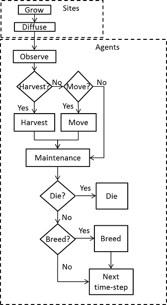
Figure 1. Model flowchart for a single time-step Table 1: Model parameters and range for sensitivity analysis Symbol Description Units/Range Nominal value Range for OFAT Range for global SA c Harvest efficiency J kg-1 0.9 0.1 – 1 0 – 1 D Diffusion coefficient km2day-1 0.1 0 – 0.25 0 – 0.25 Eb Birth energy J 6.5 1 – 10 1 – 10 Eh Harvest cost J 0.1 0 – 0.5 0 – 0.5 Em Cost of energy maintenance J 0.1 0.05 – 0.5 0 – 0.5 Emove Move cost J 0.5 0 – 2 0 – 2 K Resource carrying capacity kg 2 0.5 – 5 0 – 5 n0 Initial number of agents 0, 1, 2, ... 100 0 – 1000 0 – 400 R Resource growth rate s-1 0.1 0 – 0.5 0 – 0.5 R0 Initial resource level 0-1 (proportion of K) 1 0 – 1 0 – 1 Rmax Maximum harvest per time-step kg 0.5 0.2 – 2 0.2 – 2 Runc Uncertainty of resource estimations kg 0.1 0 – 1 0 – 1 vb Agent birth coefficient J-1 10 0 – 20 0 – 20 vd Agent mortality coefficient J-1 10 0 – 20 0 – 20 z Variation in offspring traits \([0,\rightarrow>\) 0.2 0 – 0.5 0 – 0.5 Choice of inputs and output
- 4.2
- As output of interest for the sensitivity analysis we choose the number of agents \(n\). In general it is possible to consider any number of outputs that are of interest. The methods that we discuss here, however, consider only a single output at a time. Thus, the analysis is then performed separately for each output.
- 4.3
- We include all of the model parameters and initial conditions in Table 1 as inputs for the sensitivity analysis. For those parameters that are limited to a set range we sample uniformly from this full range. For parameters that do not have a set range we choose a wide range. By testing all parameters uniformly over wide input ranges, we explore the model behaviour without imposing strong assumptions on the input parameters. We thus ensure that we do not ignore interesting model behaviour because it falls outside of the chosen input range. Since we do not a priori know how the model responds to changes in any of the parameters, it is recommended to include all model parameters in the sensitivity analysis. The initial analysis can always be supplemented with more detailed investigations of selected parameters or input ranges. The computational costs, however, can be a limiting factor to the inclusion of model parameters in the sensitivity analysis. The costs for OFAT are lower than for global sensitivity analysis, so an OFAT analysis can be used to select parameters of interest for global sensitivity analysis. Specific interests or hypotheses of the researcher can also guide the choice of inputs.
Model
results
-
Operational details
- 5.1
- The whole analysis was carried out in R (2012). The sample points for the sensitivity analysis were also generated in R. The sample points were exported to perform the model runs in Netlogo.
- 5.2
- We conduct a pre-test to determine whether the model
converges to a steady state behaviour. The pre-test consists of 1000
model runs at parameter values drawn from uniform distributions within
the range for global sensitivity analysis listed in Table 1. We record the output at every
time-step. The output initially changes strongly in time, but from
\(t=500\) to \(t=1000\) it seems to have stabilised and consist of
random fluctuations around a mean (Figure 2).
We conclude that 500 time-steps is a reasonable time period for the
sensitivity analysis, since the model output does not strongly change
between \(t=500\) to \(t=1000\). There are, however, random
fluctuations around the mean. Furthermore, runs at the nominal set show
that the number of agents oscillates in time. To prevent the output
from being strongly dependent on the random fluctuations and the phase
of the oscillations, we average \(n\) from \(t=500\) to \(t=1000\).
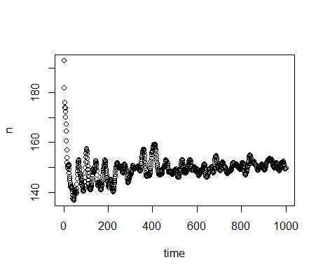
Figure 2. Plotted is the average \(n\) for 1000 model runs with parameter values randomly drawn from uniform distributions in the range for global sensitivity analysis listed in Table 1. There are strong changes in \(n\) over the first few hundred time-steps. From \(t=500\) to \(t=1000\), \(n\) seems to have converged to random fluctuations around a mean. - 5.3
- Even though the output does not change strongly between \(t=500\) to \(t=1000\), there seems to be a small and gradual increase in the mean value. This increase is caused by a gradual shift in the distribution of the agent characteristics \(w_{harvest}\) and \(w_{move}\), which affect the probabilities of harvesting or moving. This shift results from the inheritance of these characteristics during reproduction. On average, values that increase the chances of an agent to survive and reproduce are passed on more frequently. On the long-term, this causes a change in the distributions of those characteristics and this affects the number of agents supported by the environment. For the sensitivity analysis, however, we do not examine this long-term adaptivity. The chosen time-scale from \(t=500\) to \(t=1000\) is sufficiently short not to be strongly affected by the adaptivity, and sufficiently long not to depend strongly on random fluctuations and oscillations.
- 5.4
- We perform 10,000 replicate runs in the default parameter
set to estimate the distribution of the output. The stabilization of
the coefficient of variation,
$$ c_v= \frac{\sigma(n)}{\mu(n)}, $$ (7) where \(\sigma(n)\) is the standard deviation of the output and \(\mu(n)\) is the mean of the output, indicates the required number of replicates to obtain a proper estimate of the distribution of the model output (Lorscheid et al. 2012). Figure 3 shows that the coefficient of variation is largely stabilised after a few hundred replicates. The form of the distribution of \(n\) depends strongly on the parameter values. In the nominal set, the distribution over 10,000 replicates (Figure 4) has a heavy tail on the right side. At \(D=0.05\), however, the distribution resembles a normal distribution (Figure 5), whereas at \(D=0.15\) it shows a large peak at \(n=0\) (Figure 6). This peak is caused by extinction of the agent population that occurs stochastically in a region of the parameter space. We will return to this finding when we discuss the results of the OFAT sensitivity analysis.
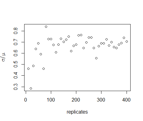
Figure 3. Coefficient of variation of the average number of agents for increasing number of replicates in the nominal parameter set. The coefficient of variation has largely stabilised after a few hundred model runs, indicating that this number is sufficient for estimation of the distribution of \(n\). - 5.5
- For the OFAT sensitivity analysis, we use 10 replicates per
parameter setting in order to roughly estimate the spread of the
output. For the regression-based sensitivity analysis, 5 replicates are
used in order to estimate the proportion of the variance of the output
that is explained by variations in the input parameters. For the Sobol'
method, we follow the usual procedure of sampling as many different
points as possible to accurately estimate the sensitivity indices (Saltelli et al. 2008). We
therefore do not use any replicates. A number of sampling designs are
available to minimise the computational costs of the estimation (e.g. Cukier et al. 1978; Tarantola
et al. 2006; Saltelli 2002). Here we
use
the design by Saltelli (2002),
with a total sample size of 17,000 model runs. This design is
relatively easy to use and it estimates all of the first- and
total-order sensitivity indices. A more detailed description of the
design is given in Appendix C.
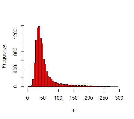
Figure 4. Histogram of 10,000 samples in the nominal set displaying the average number of agents between \(t=500\) and \(t=1000\). The distribution has a long tail for large values of \(n\). 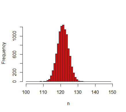
Figure 5. Histogram of 10,000 replicates for \(D=0.05\) displaying the number of agents averaged between \(t=500\) and \(t=1000\). The resulting distribution resembles a normal distribution. 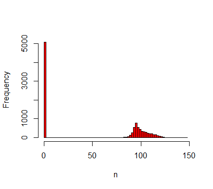
Figure 6. Histogram of 10,000 replicates for \(D=0.15\) displaying the number of agents averaged between \(t=500\) and \(t=1000\). The resulting distribution is split between a peak at \(n=0\) and a distribution around \(n=100\). The peak is caused by stochastic extinction that occurs for some values of \(D\) (see OFAT results). One-factor-at-a-time sensitivity analysis
- 5.6
- We perform OFAT sensitivity analysis for all of the model parameters. The default values and ranges of variation of all parameters are listed in Table 1. We run the model for the extreme values of this range and 9 equidistant points in between. The resulting graph for the diffusivity (Figure 7) shows two tipping points where the number of agents goes to zero. When \(D=0\), sites without resource cannot be replenished through diffusion from neighbouring sites, eventually leading to collapse of the system. Inspection of the time-series of a number of model runs reveals that the number of agents oscillates with increasing amplitude for increasing values of \(D\). Between \(D=0.10\) and \(D=0.15\) this amplitude becomes so large that \(n\) crosses zero, causing the system to collapse. Because the model is stochastic, this collapse occurs in some but not all of the replicates. Tests with simulation times longer than 1000 time-steps show that between \(D=0.10\) and \(D=0.15\) extinction occurs mostly during the first 1000 time-steps. If extinction does not occur during this initial period, then n remains positive on the long term. The model thus has multiple equilibria for these parameter values. For \(D \leq 0.175\) the population always goes to extinction, but for \(D=0.175\) it sometimes takes more than 1000 time-steps before this equilibrium is reached. One of the model runs in Figure 7 therefore still has a positive population after 1000 time-steps.
- 5.7
- The graphs for the other parameters are shown in Appendix
B. Out of a total of 15 model parameters, 11 parameters show a tipping
point where the number of agents goes to zero. Furthermore, most
parameters show a nonlinear response when the number of agents is
positive. The graphs yield mechanistic understanding of the model. We
pick a few parameters for a brief discussion. For higher values of
\(r\), the resource replenishes faster and the system supports a larger
number of agents. The carrying capacity \(K\) also has a positive
effect on the number of agents, but higher values destabilise the
system and cause collapse of the population. Low values for the energy
costs required for maintenance \(E_m\) and for harvesting
\(E_{harvest}\) also lead to collapse by causing an increase in the
amplitude of the oscillations of the number of agents. High values of
\(E_m\) and \(E_{harvest}\) lead to lower agent numbers because the
system is able to support less agents if those agents require more
energy. A high energy cost for moving \(E_{move}\), however, does not
lead to low agent numbers. For high move costs, the agents will simply
move less often and instead decide to harvest at their current
position. The initial conditions \(n_0\) and \(R_0\) can affect the
final state of the system by causing an early collapse, but have no
effect on the final state if the number of agents remains positive.

Figure 7. Results of the OFAT analysis for \(D\). Displayed are the mean (green circle), minimum (red triangle) and maximum (blue cross) of the number of agents among 10 replicates. The dashed line represents the nominal value. Regression-based sensitivity analysis
- 5.8
- The regression-based global sensitivity analysis is based on Nr=1000 sample points drawn from uniform probability distributions over the range given in Table 1. The range for the initial number of agents for global sensitivity analysis is smaller than for OFAT. Using the same range as the OFAT, the number of agents reaches zero in almost 90% of the model runs. Extinction of the agent population is an important model outcome and we are therefore interested in understanding the conditions under which extinction takes place. However, to assess the parameter sensitivity indices we need a sufficient number of runs with nonzero outcome. We therefore reduce the range for \(n_0\) for the global sensitivity analysis. The reduced range has a larger number of runs with positive outcomes, but also contains runs where the population goes extinct.
- 5.9
- For each sample point, we use 5 replicate runs to estimate the variation of the model output due to stochasticity. To limit the computational expense this number of replicates is smaller than the 10 replicates for the OFAT. The mean output variance over replicates is 0.88% of the output variance over all samples. The variance due to stochasticity is thus negligible compared to the variance due to parameter variations and unexplained variance cannot be attributed to the stochasticity inherent in the model. Since the variance due to stochasticity is so small, we do not need a more accurate estimate of this variance, which gives us confidence that we do not need to increase the number of replicate runs per parameter setting.
- 5.10
- We fit a first-degree polynomial (Equation 8) of the model
parameters \(x_i\) to the output using ordinary least squares
regression (OLS),
$$ n = b_0 + \sum_i^m b_i x_i . $$ (8) - 5.11
- The outcomes show that the total number of 5000 model runs was sufficient to obtain reasonably accurate estimates of the explained variance and the first-order sensitivity indices (Table 2). However, the coefficient of determination \(R^2 =43.9 \pm 4.1\)% (Table 2) shows that more than half of the model variance is unexplained. We attempt to increase the explained variance by adding higher order terms to Equation 8. We distinguish between terms that are nonlinear in a single parameter \(x_ix_i\) and interaction terms \(x_ix_j\). Table 3 lists the values of \(R^2\) for a number of functions that are obtained by adding such terms. The increase in explained variance should be weighed against the increase in the complexity of the regression model. Functions with a large number of terms will generally yield high values of \(R^2\) simply due to the larger number of degrees of freedom. Table 3 shows that even with a very large number of terms a large part of the model variance still remains unaccounted for. Furthermore, such a large number of terms is not useful in terms of gaining insight into the influential model processes. A common alternative to fitting a first-degree polynomial (Equation 8) is fitting the logarithm of the parameter instead of the parameter itself. Doing this for some of the model parameters increases the value of \(R^2\) (\(R^2 = 48.1\)%). However, the increase is only small compared to a polynomial fit and still leaves a large part of the variance unexplained.
- 5.12
- Figures 4-6 show that the form of distribution of \(n\)
depends on the parameter values. The distribution over the \(N_r=1000\)
samples used for the regression-based sensitivity analysis (Figure 8)
contains a large peak at \(n=0\) and a long tail with a number of
outliers for large values of \(n\). For these kind of asymmetric
distributions, OLS, which assumes normally distributed residuals, does
not generally produce good fits (Draper
& Smith 1998).
Specifically, outlying values relative to the normal distribution tend
to destabilize the regression function. The explained variance \(R^2\)
is then no longer a good measure. This presents a possible explanation
for the failure to obtain a good fit. Moreover, the outliers that
destabilize the OLS regression weigh heavily in the variance itself.
This is illustrated by Figure 9,
which visualizes the contributions of different sample points to the
variance. On the horizontal axis, the sample points are sorted by
increasing value of the output \(n\). For each point we plot the
partial sum of the squared deviations from the mean, where the mean is
computed over all sample points. The slope of the graph in a point
measures the contribution of that sample point to the variance. The
slope is initially straight, because a large number of sample points
with outcome \(n=0\) contribute equally to the variance. Each coloured
area corresponds to 25% of the total variance. Outlying values
represent a large amount of the total variance. Out of \(N_r=1000\)
samples, the 14 highest values represent 25% of the variance, and the
61 highest values represent 50% of the variance. The dashed line
represents the explained variance by the regression model (Equation 8).
The regression model does not adequately capture the contribution of
outliers to the variance. The outliers give valuable information on the
extreme cases of model behaviour and the conditions under which such
extreme behaviour occurs. It is therefore important to consider these
outliers as part of sensitivity analysis. However, since these outliers
represent a major part of the variance, any sensitivity analysis method
based on variance decomposition will assign them a disproportionate
weight.
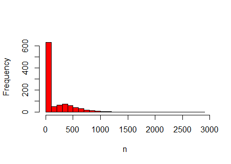
Figure 8. Histogram of the number of agents, for the \(N_r=1000\) sample points used for the regression-based sensitivity analysis. The histogram shows a large peak at \(n=0\) and contains a number of outliers between \(n=1000\) and \(n=3000\). 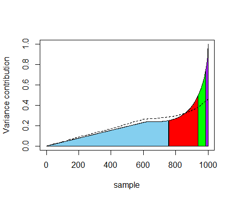
Figure 9. Contribution to the variance of each sample for the regression-based sensitivity analysis. The sample points are sorted by increasing output \(n\). The variance contributions are then computed as the partial sum of squared deviations from the mean, assuming the mean to be constant. The values are normalised by the total variance. Each colour represents 25% of the total variance. For the dashed line, the output for each sample is replaced by the predicted output of the regression model (Equation 8). A small number of outliers on the right contributes strongly to the total variance, but this contribution is not adequately captured by the regression model. Table 2: First-order indices according to Equation 8. The confidence intervals are based on a bootstrap sample of size 10,000. Only parameters with at least 1.0% explained variance are included. We also report the standardized regression coefficients \(\beta_i =b_i\sigma (n)/\sigma (x_i)\). Here the standard deviation \(\sigma(n)\) is computed from the output sample of the sensitivity analysis and the standard deviation \(\sigma(x_i)\) is given by the input distribution of the parameter \(x_i\) (see e.g. Cariboni et al. 2007). The standardized regression coefficients measure the strength as well as the direction of the effect of the parameter on the output. Parameter k r Em Rmax Eh c D Total Sr 20.0% ±3.8% 9.1% ±3.0% 5.7% ±2.6% 4.1% ±2.2% 3.3% ±1.9% 1.6% ±1.4% 1.0% ±1.2% 45.5% ±4.1% \(\beta\) 0.43 0.29 −0.24 0.23 −0.18 0.23 0.10 - Table 3: \(R^2\) for various polynomial regression models with increasing number of terms. A significant increase in the explained variance is obtained by adding terms to the regression model, but this should be weighed against the increased complexity of the regression model. The table shows a large number of terms is needed to significantly increase the explained variance. order of nonlinearities 1st 2nd 3rd 1st 2nd 1st 2nd 3rd order of interactions - - - 2nd 2nd 3rd 3rd 3rd number of coefficients 16 31 46 121 136 576 591 606 \(R^2\) 45.5% 49.9% 51.2% 63.7% 67.7% 65.5% 69.0% 70.0% Sobol' method
- 5.13
- The computation of the Sobol' main and total-order sensitivity indices was carried out using the sampling scheme by Saltelli (2002) with a total sample size of 17,000 model runs. We used uniform distributions in the range given in Table 1. The resulting first- and total-order indices are shown in Figure 10. We assess the accuracy of the estimated sensitivities using bootstrap confidence intervals, based on 10,000 bootstrap samples (Archer et al. 1997). Some of the intervals are wide, showing that the estimate is not accurate. Furthermore, a number of the confidence intervals contain negative values. These negative ranges have no valid interpretation because the sensitivity represents a portion of the model variance, which is bound between 0% and 100%. The sensitivity estimates, however, can be negative due to numerical inaccuracy of the method (Saltelli et al. 2008). Thiele et al. (2014) report the same finding, but discard the negative ranges by setting them to zero. However, this introduces a bias in the bootstrap confidence interval. For example, in our results the sensitivity of the parameter \(E_b\) has a wide confidence interval that spans mostly negative values. If we discard these negative values, then the sensitivity would appear to be estimated at zero with a very high precision. We therefore report the negative values. Appendix C provides a more detailed explanation of these negative outcomes.
- 5.14
- The sum of all first-order indices equals 0.46. This
includes both linear and nonlinear contributions of individual
parameters, but no interaction effects. More than half of the model
variance is thus explained by interaction effects according to the
variance decomposition of Equation 4. The total-order indices show that
a number of parameters explain little variance even including
interaction effects. Additionally, the more influential parameters have
wide confidence intervals for the total-order sensitivities. We thus
have only rough estimates of the amount of variance those parameters
can explain including their interactions. However, a few parameters,
such as \(K\) and \(R_{max}\) are clearly influential, because even the
lower ends of the confidence intervals of the total-order sensitivities
are large compared to the sensitivity estimates of other parameters.
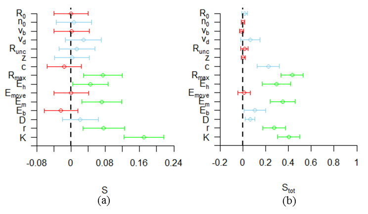
Figure 10. First-order (a) and total-order (b) Sobol' indices for all parameters. The colours categorize the parameters from most influential (green) to averagely influential (blue) and least influential (red).
Discussion
- 6.1
- We have applied three commonly employed methods of sensitivity analysis to a typical but low-complexity ABM. Here we evaluate each method in terms of our three selected aims (1/ understanding the emergence of patterns, 2/ evaluating robustness, and 3/ evaluating outcome uncertainty). Table 4 summarizes the outcomes of this evaluation. We will discuss the Table in more detail below.
- 6.2
- The OFAT method yields insight into qualitative aspects of model behaviour and the patterns that emerge from the model. It gives important information about the functional form of the relationships between parameters and output variables. Furthermore, it shows the existence of tipping points and other strong nonlinearities. Exposing such qualitative aspects can lead to a better mechanistic understanding of the behaviour of the model and thus the modelled system. OFAT can also be used to show the robustness of model behaviour with respect to changes in single parameters, thus revealing whether emergent patterns depend on strong assumptions. Interaction effects are not considered, and therefore OFAT is not suitable for further quantification of sensitivity indices. OFAT should therefore be supplemented by some global method of sensitivity analysis to examine interaction effects and to quantify model variability that results from parameter variations. For our case, for example, global sampling from the parameter space revealed that interaction effects lead to the existence of outliers for which the output takes extreme values. Since each parameter is only varied individually and not in combination with other parameters, OFAT is relatively cheap in terms of computational costs. At 10 replicates for 11 parameter values, we need 110 model runs per parameter, or 1650 runs in total. This cost could still be lowered by decreasing the number of replicates.
- 6.3
- Regression-based sensitivity analysis is a global method based on variance decomposition. A major limitation for application to sensitivity analysis of ABMs is that it depends on the structure of the model whether a good decomposition can be obtained by regression. In our case a good fit (with \(R^2>0.9\)) was not obtained even using a third-order polynomial function because of the existence of outlying values as well as regions of parameter space where the output goes to zero. This corresponds to previous reporting difficulties by Burgers et al. (2010) on finding a good fitted function for an ABM of trading agents. They attributed these difficulties to the inherent complexity of the model. We agree with this assessment, where we explicitly add that in our case the lack of fit is better understood by considering the results we obtained by first performing the OFAT. The lack of fit resulting from the inherent complexity of ABMs limits the usefulness of regression-based sensitivity analysis for these models, as the systems which they are used to model are complex adaptive systems that are characterized by the existence of nonlinear interactions and feedbacks, multiple levels of model behaviour, and emergent properties. These characteristics complicate and obscure the relations between the model inputs and outputs and are thus not straightforwardly captured by a regression function. Even though the regression function does not yield a good fit, however, regression-based sensitivity analysis might prove useful in selecting influential parameters for further analysis based on the sensitivity indices or regression coefficients. The computational costs of regression-based sensitivity analysis lie somewhere in between OFAT and the Sobol' method. For our test-case 1000 parameter settings with 5 replicates each were sufficient to obtain reasonably accurate estimates of the first-order indices.
- 6.4
- The Sobol' method does not use fitted functions, but instead decomposes the variance based directly on a sample from the parameter space (Saltelli et al. 2008). The method aims to quantify the output variability based on this variance decomposition. Whereas the variance has a clear interpretation for normal distributions, it is not a good measure of variability for distributions that are skewed or contain outliers (Swinscow 1997). This problem is illustrated by Figure 9, which shows that the output variance of our test case is inflated by a few outlying sample points. The method is therefore not suitable for quantifying outcome variability of ABMs with output distributions that have outliers, are skewed, or strongly deviate in other ways from the normal distribution (Liu et al. 2006). Another drawback of the method is that the method does not allow for the possibility to distinguish between mechanistic explanations on why a parameter is influential. For example, in our test case the harvesting cost \(E_h\) shows up as an influential parameter (Figure 10b), but it is unclear whether it has some effect on outlying values, or causes collapse of the population, or affects the number of agents for positive population sizes. In contrast, the OFAT results show that \(E_h\) causes population collapse and affects the number of agents for positive populations, but such specific findings are lost in the Sobol' method because sensitivities are aggregated over the full parameter space (Rakovec et al. 2014). As such, the method also does not reveal the robustness of model patterns to parameter changes within this space. Out of the methods we tested, the Sobol' method has the largest computational costs. With a total of 17.000 model runs, the estimates of the sensitivity indices have wide confidence intervals. For a number of parameters these intervals included negative values, which have no valid interpretation.
- 6.5
- In light of these results we recommend OFAT as the starting
point for any sensitivity analysis of an ABM, in particular when one
wants to gain insight into the mechanisms and patterns that ABMs
produce, which is a typical goal of many social simulation studies.
This recommendation seemingly contradicts the one by Saltelli et al. (2008) and Ligmann-Zielinska
et al. (2014),
who suggest the use of the Sobol' method for model analysis. However,
our study suggests that standard methods of global sensitivity analysis
do not adequately address the issues that are relevant for the analysis
of ABMs, such as the existence of multiple levels, nonlinear
interactions and feedbacks, and emergent properties, as effectively as
OFAT. Obviously any OFAT can be supplemented with a global method to
investigate interaction effects, given that certain conditions are met,
namely that the output distribution is and remains sufficiently similar
to a normal distribution, regression fits have a high \(R^2\), and
confidence intervals have positive bounds. Some promising advancements
in other fields might prove useful for ABM applications. These include
a hybrid local-global sensitivity method that examines the distribution
of explained variances over portions of the parameter space (Rakovec et al. 2014) and
alternative sensitivity measures based on entropy instead of variance (Liu et al. 2006; Auder &
Iooss 2009).
Table 4: Evaluation of three different methods of sensitivity analysis in terms of different aims. Aim Method Evaluation Rating Examine patterns OFAT Shows the effect of individual parameter changes on emergent patterns. Gives insight into model mechanics by revealing tipping points and other nonlinearities. +
Regression-based Condenses ABM output into descriptive relationships, which yield insight into model behaviour. However, the relationships are valid only if the regression model fits well to the ABM. +/-
Sobol' Considers only the averaged effect of parameters over the whole parameter space, and therefore does not explore different patterns within this space. - Examine robustness OFAT Shows robustness of patterns to individual parameter changes. However, interaction effects are not included. +/-
Regression-based If a good fit is found, then the descriptive relationships give insight into the robustness and can account for interaction effects. +/-
Sobol' Does not investigate the robustness of certain outcomes, only the effects - Quantify outcome variability due to parameters OFAT Does not examine this variability, because this requires consideration of interaction effects. -
Regression-based If a good fit is found, then the output variance is decomposed into terms attributed to different (combinations of) parameters. +/-
Sobol' Decomposes the output variance into terms attributed to different (combinations of) parameters. +/-
Appendix A. Model description
-
The model description follows the ODD (Overview, Design concepts, Details) protocol for describing individual- and agent-based models (Grimm et al. 2006, 2010).
1. Purpose
The basic topic of the model is how individual agents in a spatial environment make trade-offs between conserving energy by remaining inactive and becoming active to gather energy. Energy is gathered from the environment and spent on a daily maintenance that represents the physiological processes of the agent and on the actions of moving and harvesting.
2. Entities, state variables, and scales
The state variables are listed in Table A1. The landscape is represented by a square lattice of length \(L\). Each site \(i,j(i,j=1,2,\ldots,L)\) has a length of \(\Delta x=1\)km. Since the model was not fitted to realistic data, this choice is to some extent arbitrary. Setting \(\Delta x=1\), is convenient for computations with parameters that have length-units in their dimensions. Periodic boundary conditions are imposed, so that \(i+L=i\) and \(j+L=j\). Each site has a resource level \(R_{i,j}\).
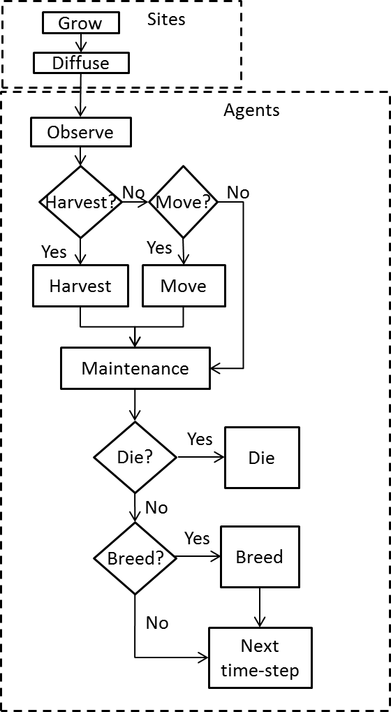
Figure A1. Flowchart for a single time-step Agents move over the lattice and harvest resource. An agent is identified by the index \(a=1,2, \ldots\). Each agents has an energy level \(E^a\) and a location \(x^a\). Agents estimate the resource levels at their site and at the four Von Neumann nearest neighbour sites every time-step. Thus, an agent with location \(x^a=i,j\) has estimates for \(R_{i,j}\), \(R_{i\pm1,j}\) and \(R_{i,j\pm1}\). Agents also have harvest and move coefficients, \(w_h^a\) and \(w_m^a\). Agents with a high value for \(w_h^a\) or \(w_m^a\) are less likely to harvest resource or move to a neighbouring site respectively. The values of \(w_h^a\) and \(w_m^a\) are constant for each agent.
Time is modelled in discrete time steps of \(\Delta t=1\) day. Like the distance scale of \(\Delta x=1\), this was chosen to make computations convenient.
Table A1: State variables. The upper part of the table contains the site state variables. The lower part contains the agent state variables. Symbol Description Dimensions Range \(i,j\) Position indices - \(0,1,\ldots,L ; 0,1,\ldots,L\) \(R_{i,j}\) Resource kg \([0,\rightarrow>\) \(R_{i,j}^{a}\) Estimated resource kg \([0,\rightarrow>\) \(x^a\) Position - \((0,1,...,L;0,1,...,L)\) \(a\) Agent index - \(0,1,2,...\) \(w_h^a\) Harvest coefficient - \([0,\rightarrow>\); \(w_m^a\) Move coefficient - \([0,\rightarrow>\) 3. Process overview and scheduling
The model flow chart for a single time-step is shown in Figure A1. The submodels in the boxes are described in detail in the submodel section. Each submodel is run for all of the patches/agents before the start of the next submodel.
The time-step starts with the updating of the sites. The 'grow' submodel grows resource on each site following a logistic growth equation. The 'diffuse' submodel diffuses the resource between sites following Fick's second law (Fick 1855).
The updating of sites is followed by the agent actions. Each agent first 'observes' the resource level and the number of agents on neighbouring sites. The agents then decide whether to harvest, based on their internal energy state, the estimated resource level on their location, and the presence of other agents. If an agent does not harvest, it may decide to move based on the number of agents and estimated resource level on neighbouring sites. Alternatively, an agent may decide to neither harvest nor move, thus conserving energy. After all the agents have decided, the actions of harvesting and moving are carried out in random order. Each agent then pays a fixed energy maintenance. The internal energy state of each agent affects the probabilities of dying and breeding. The model then proceeds to the next time-step.
4. Design concepts
-
Basic principles
The model considers agents that move and harvest in a spatial environment. Based on their internal state and the state of the environment agents may decide to move to a new location, to harvest from the present location, or to wait for a better opportunity. Harvested resource is converted to internal energy, which is used to pay daily maintenance. The energy for maintenance The acts of moving and harvesting also cost energy. The decisions to move and harvest are based on both the internal energy state of the agent and the state of the environment.
Emergence
We consider the total population size \(n_{tot}\) and the values of the harvest and move coefficients \(w_h^a\) and \(w_m^a\) averaged over the population as emerging variables at the macro-level.
Adaptation
Agents adapt their behaviour to changes in their internal state or in their environment. Agents with low levels of internal energy tend to harvest resource with a higher probability. Agents also tend to harvest if the resource level on their site is high and the number of other agents on the site is low.
Agents consider the state of the sites in the Von Neumann neighbourhood in their decisions to move to neighbouring sites. Agents are more likely to harvest if the resource level on their current site is high and there are few other agents on this site. Agents are more likely to move to sites with high resource levels and few other agents.
Objectives
The first objective of each agent is to gather sufficient resource to ensure its own survival. The second objective is to accumulate sufficient energy to breed.
Learning
Individual agents do not change their adaptive traits over time. However, the distribution of these traits over the population may change due to selection. When agents breed, their offspring inherit the parents' values of \(w_h^a\) and \(w_m^a\) with some random variation. If, for example, agents with a low value \(w_m^a\) reproduce more frequently often on average, then low values will become increasingly common over time.
Prediction
Agents tend to move less often to sites that are occupied by one or more other agents, based on the prediction that those other agents may harvest resource from the site. Agents tend to harvest more often at their present location if neighbouring locations are occupied by other agents that might move to the resource. Agents also tend to move to sites with high resource levels, predicting that the resource level will remain high and can be harvested. If an agent finds the present conditions unsuitable for harvesting, that agent may decide to wait before taking action, expecting that the conditions will improve in the future.
Sensing
Agents sense their own internal energy. Each time step, agents assess the amount of resource on their current location and the four sites that compose the Von Neumann neighbourhood. However, agents do not sense the exact amount of resource because there is some random error. Agents also sense the presence of any other agents within the Von Neumann neighbourhood, without any error.
Interaction
Indirect interactions between agents occur through the competition for resource. In addition, agents are less likely to move to or harvest at sites that contain other agents. This is a form of direct interaction. Agents are also more likely to harvest on their present site if neighbours are occupying the neighbouring sites. The basic model formulation does not include further direct interactions between agents in order for the model to function as a benchmark.
Stochasticity
The decisions of agents to harvest at the present location or to move to a neighbouring site are based on smooth probability functions. The functions take as input the number of agents and the perceived amount of resource within the Von Neumann neighbourhood. The perceived amount of resource differs from the actual amount by an amount that is drawn from a normal distribution. Birth and death of agents are also stochastic, but based on the internal energies of agents. If an agents breeds, the offspring inherit the values of \(w_h^a\) and \(w_m^a\) with a small random variation. Furthermore, the agents' initial locations, energies and values of \(w_h^a\) and \(w_m^a\) are also stochastic.
Observation
Three output variables are collected: the total number of agents \(n\) and the averages of \(w_h^a\) and \(w_m^a\) over all agents. All output variables are recorded at each time-step.
5. Initialization
All sites are initialized with resource levels equal to \(R_0\) times carrying capacity. The initial number of agents is specified as a parameter, \(n_0\). Each agent is placed on a random site with an internal energy that is drawn from a uniform distribution between 0 and the minimum energy that is needed for procreation. The initial values of \(w_h^a\) and \(w_m^a\) are drawn from a uniform distribution between 0 and 1. The default parameter values of the model are listed in Table A2.
Table A2: List of used symbols in the model description. The upper part contains general notation, the middle part model variables and the lower part model parameters Symbol Description Units/range Default value \(i,j\) Site indices \(1,2,...,L\) - \(L\) Lattice size - 33 \(T\) Time index day - \(A\) Agent index - - \(\Delta t\) Time-step size day 1 \(\Delta x\) Site length km 1 \(E^a\) Initial energy J - \(E_{exp,i,j}^a\) Expected harvest
J
-
\(N\) Total number of agents \(0,1,2, ...\) - \(n_{i,j}\) Number of agents on site \(i,j\) \(0,1,2, ...\) - \(R_h\) Harvested resource kg - \(R_{i,j}\) Resource on site i,j kg - \(R_{i,j}^a\) Observed resource by agent \(a\) kg - \(w_h^a\) Harvest coefficient - - \(w_m^a\) Move coefficient - - \(x^a\) Location of agent \(a\) \((0,1,...L;0,1,...L)\) - \(c\) Efficiency J kg-1 0.9 \(D\) Diffusion coefficient km2day-1 0.1 \(E_b\) Birth energy J 5 \(E_h\) Harvest cost J 0.1 \(E_m\) Cost of energy maintenance J 0.1 \(E_{move}\) Move cost J 0.5 \(K\) Carrying capacity kg 2 \(n_0\) Initial number of agents 0,1,2, ... 100 \(r\) Growth rate s-1 0.1 \(R_0\) Initial resource 0-1 (proportion of K) 1 \(R_{max}\) Maximum harvest kg 0.5 \(R_{unc}\) Uncertainty of resource estimations kg 0.1 \(v_b\) Birth coefficient J-1 10 \(v_d\) Mortality coefficient J-1 10 \(z\) Variation in offspring traits \([0,\rightarrow>\) 0.2 6. Input data
The model does not use input data to represent time-varying processes.
7. Submodels
-
7.1 Grow resource
Resource grows on sites according to a logistic growth equation,$$ \frac{dR_{i,j}}{dt} = R_{i,j}r \left( 1- \frac{R_{i,j}}{K}\right) . $$ (A1) Each time-step the sites are updated using the analytical solution of this equation,
$$ R_{i,j} = \frac{R_{i,j}^{\ast} K e^{r\Delta t}}{K+R_{i,j}^{\ast} e^{r\Delta t}} . $$ (A2) Note that several processes can change the resource on a site during the same time-step. In order to keep the notation simple, we use \(R_{i,j}^{\ast}\) to denote the resource before the update in each of these processes, instead of having different symbols for the resource before and after each of the separate processes.
7.2 Diffuse resource
The resource diffuses following Fick's second law (Fick 1855),
$$ \frac{dR_{i,j}}{dt} = D \nabla^2 R_{i,j} $$ (A3) with \(\nabla=(\partial/\partial x, \partial/\partial y)\). The equation is discretised in space using the central difference and discretised in time using a forward Euler algorithm. This yields,
$$ R_{i,j} = \left( 1- \frac{4\Delta t}{\Delta x^2} D \right) R_{i,j}^{\ast} + \frac{\Delta t}{(\Delta x^2)} D \sum_{\langle nn \rangle} R_{i',j'}^{\ast} $$ (A4) where the sum runs over the 4 nearest neighbours. It is shown by Von Neumann stability analysis that the solution is stable for \(\Delta t/\Delta x^2 D < 1/4\).
7.3 Observe
Agents estimate the resource levels on their present location and the 4 Von Neumann nearest neighbours. The difference between the estimated and the actual amount is drawn from a normal distribution with mean 0 and standard deviation determined by the parameter \(R_{unc}\).
$$ R_{i,j}^a = R_{i,j} + \Delta R $$ (A5) with \(R_{i,j}^a\) the estimated amount, \(R_{i,j}\) the actual amount and the difference \(\Delta R \sim N(0,R_{unc})\). The result of the observation is stored by the agent until it is replaced by the next observation.
7.4 Harvest?
The decision of whether to harvest is based on the current internal energy of the agent and the amount of resource that the agent estimates to be present on the site. The current internal energy is compared with the energy maintenance per time-step,
$$ H(E^a) = \frac{E^a}{E_m} -1. $$ (A6) A small value of \(H\) indicates that the agent has a low internal energy and needs to harvest soon (i.e. the agent is hungry). If \(H\) is negative, then the agent must harvest to survive for another time-step. An agent compares perceived resource on its present site to the maximum possible harvest \(R_{max}\), which is constant,
$$ G(R_{i,j}^{\ast a}, n_{i,j}) = 1- \frac{R_{i,j}^{\ast a}}{n_{i,j} R_{max}} . $$ (A7) The resource that the agent expects to harvest is given by the estimated amount of resource on the patch divided by the total number of agents on the patch. If \(G\) is close to 1, then the expected harvest is small. If \(G\) is close to zero, then the agent expects to harvest close to the maximum possible amount. The final probability to harvest is computed based on the functions \(H\) and \(G\),
$$ P_{harvest}^a = e^{-w_h^a HG}, $$ (A8) where \(w_h^a\) represents the internal tendency of the individual agent to harvest. Thus an agent is likely to harvest if it is hungry, if it sees a good opportunity for making a harvest, and if it has a high internal tendency. Since the functions \(H\) and \(G\) are dimensionless, the state variable \(w_h^a\) is also dimensionless. Note that the probability of harvesting goes to one if the agent is very hungry, or if the expected harvest is equal to the maximum possible harvest.
7.5 Move?
When deciding whether or not to move, an agent predicts how much resource it expects to obtain at its current site and at the four nearest neighbouring sites. For its current site \(i,j\) the agent expects that the resource will be shared evenly among the agents on that site,
$$ E_{exp,i,j}^a = \frac{cR_{i,j}}{n_{i,j}}. $$ (A9) For a neighbouring site, the agent expects that it will share the resource with the agents already present at the site. The agent also considers that it will first have to spend energy to move to a neighbouring site before harvesting there. Thus, the net expected energy gain for the neighbouring site is equal to the expected harvest minus the cost of moving to the site,
$$ E_{exp,k,l}^a = \frac{cR_{k,l}}{n_{k,l}} -E_{move} . $$ (A10) The expected energy gain of the current site is then compared with that of the nearest neighbour with the highest expected gain. Based on this comparison, the probability of moving is computed
$$ P_{move} = e^{-w_m^a E_{i,j}/E_{k,l}} $$ (A11) Thus, an agent is likely to move if the expected energy gain is higher on a neighbouring site than on the present location. Since both the expected harvests have the dimensions of energy, the variable \(w_m^a\) is dimensionless. This variable represents the differences between agents in their likeliness to move.
7.6 Harvest
The harvest is carried out by updating the amount of resource on the harvested site \(i,j\) and the internal energy level of the harvesting agent. The agent harvests any resource present on the site up to a maximum of \(R_{max}\). The new amount of resource is thus \(R_{i,j}=R_{i,j}^\ast-R_h\), with \(R_{i,j}^\ast\) the amount before harvesting and \(R_h\) the harvested amount,
$$ R_h= \left\{ \begin{array}{ll} R_{i,j}^\ast& \quad \mathrm{if}~R_{i,j}^\ast< R_{max},\\ R_{max} & \quad \mathrm{if}~R_{i,j}^\ast> R_{max} .\\ \end{array}\right.$$ (A12) The cost of harvesting \(E_h\) is deducted from the internal energy of the agent and the harvested resource is converted with efficiency \(c\) and added to the internal energy,
$$ E^a = E^{\ast a} + cR_h-E_h . $$ (A13) 7.7 Move
The agent moves to the nearest neighbour with the highest value of \(R_{i,j}^a/n_{i,j}\). The location of the agent is updated to the new site.7.8 Maintenance
For each agent, the daily energy cost of maintenance is deducted from the internal energy,$$ E^a=E^{\ast a}-E_m . $$ (A14) If the internal energy of the agent is lower than the maintenance costs, it will become negative after paying maintenance. Because the 'pay maintenance' submodel is immediately followed by the 'die?' submodel, the agent will then die without taking any further actions.
7.9 Die?
Every time-step, agents have a probability of dying or breeding, based on their internal energy. The probability of dying is
$$ P_{die}(E^a)=e^{-v_d E^a}. $$ (A15) Thus, the probability of dying goes to one as \(E^a\) goes to zero.
7.10 Die
If an agent dies it is removed from the simulation.
7.11 Breed?
If an agent does not die, it has a probability of breeding,
$$ P_{breed}(E^a)= 1-e^{-v_b (E^a-E_b)}. $$ (A16) If \(E^a < E_b\) then the probability is set to zero. The submodel determines whether the agent will breed based on this probability.
7.12 Breed
If an agent breeds, it is replaced by two new agents. The energy of the parent is split evenly among the two offspring. The values of \(w_h^a\) and \(w_m^a\) are inherited by the offspring with some random deviation. The deviation is drawn from a uniform distribution between \(-z\) and \(z\). In some cases, the resulting value of \(w_h^a\) and \(w_m^a\) can be negative. It is then set to zero instead.
Appendix B: OFAT results
-
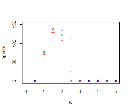
Figure B1. Results of the OFAT analysis for \(K\). Displayed are the mean (green circle), minimum (red triangle) and maximum (blue cross) of the number of agents among 10 replicates. The dashed line represents the nominal value. 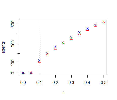
Figure B2. Results of the OFAT analysis for \(r\). Displayed are the mean (green circle), minimum (red triangle) and maximum (blue cross) of the number of agents among 10 replicates. The dashed line represents the nominal value. 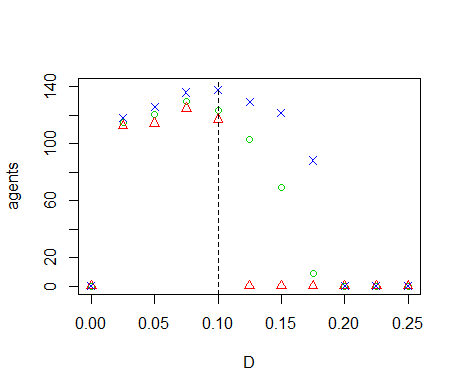
Figure B3. Results of the OFAT analysis for \(D\). Displayed are the mean (green circle), minimum (red triangle) and maximum (blue cross) of the number of agents among 10 replicates. The dashed line represents the nominal value. 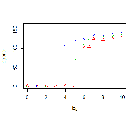
Figure B4. Results of the OFAT analysis for \(E_b\). Displayed are the mean (green circle), minimum (red triangle) and maximum (blue cross) of the number of agents among 10 replicates. The dashed line represents the nominal value. 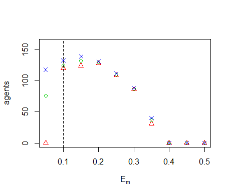
Figure B5. Results of the OFAT analysis for \(E_m\). Displayed are the mean (green circle), minimum (red triangle) and maximum (blue cross) of the number of agents among 10 replicates. The dashed line represents the nominal value. 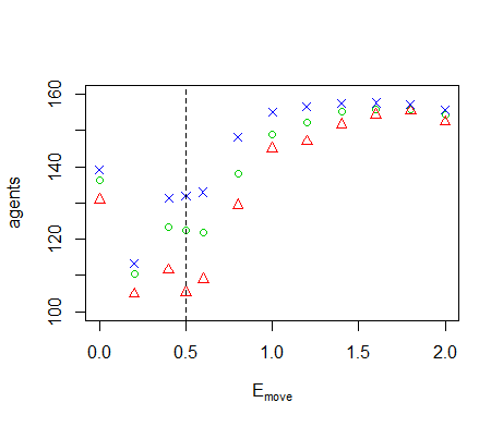
Figure B6. Results of the OFAT analysis for \(E_{move}\). Displayed are the mean (green circle), minimum (red triangle) and maximum (blue cross) of the number of agents among 10 replicates. The dashed line represents the nominal value. 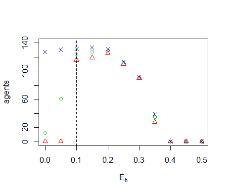
Figure B7. Results of the OFAT analysis for \(E_h\). Displayed are the mean (green circle), minimum (red triangle) and maximum (blue cross) of the number of agents among 10 replicates. The dashed line represents the nominal value. 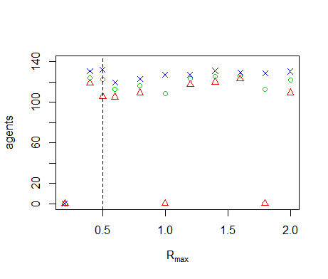
Figure B8. Results of the OFAT analysis for \(R_{max}\). Displayed are the mean (green circle), minimum (red triangle) and maximum (blue cross) of the number of agents among 10 replicates. The dashed line represents the nominal value. 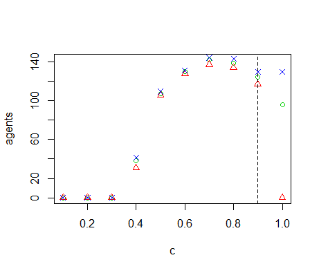
Figure B9. Results of the OFAT analysis for \(c\). Displayed are the mean (green circle), minimum (red triangle) and maximum (blue cross) of the number of agents among 10 replicates. The dashed line represents the nominal value. 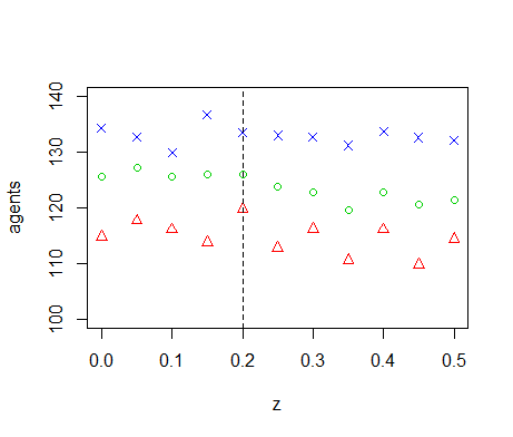
Figure B10. Results of the OFAT analysis for \(z\). Displayed are the mean (green circle), minimum (red triangle) and maximum (blue cross) of the number of agents among 10 replicates. The dashed line represents the nominal value. 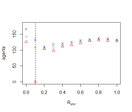
Figure B11. Results of the OFAT analysis for \(R_{unc}\). Displayed are the mean (green circle), minimum (red triangle) and maximum (blue cross) of the number of agents among 10 replicates. The dashed line represents the nominal value. 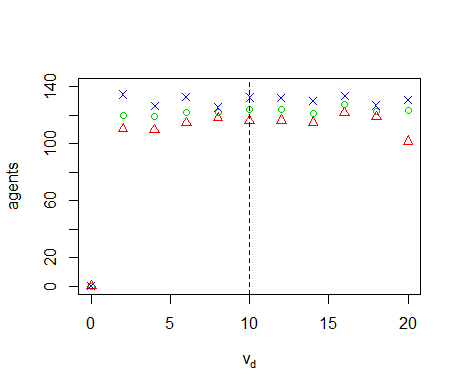
Figure B12. Results of the OFAT analysis for \(v_d\). Displayed are the mean (green circle), minimum (red triangle) and maximum (blue cross) of the number of agents among 10 replicates. The dashed line represents the nominal value. 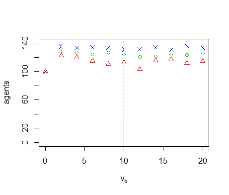
Figure B13. Results of the OFAT analysis for \(v_b\). Displayed are the mean (green circle), minimum (red triangle) and maximum (blue cross) of the number of agents among 10 replicates. The dashed line represents the nominal value. 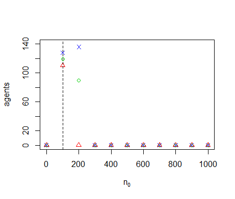
Figure B14. Results of the OFAT analysis for \(n_0\). Displayed are the mean (green circle), minimum (red triangle) and maximum (blue cross) of the number of agents among 10 replicates. The dashed line represents the nominal value. 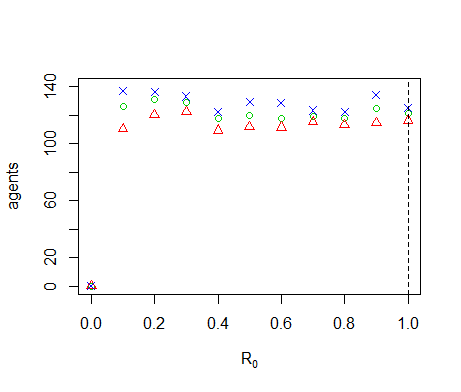
Figure B15. Results of the OFAT analysis for \(R_0\). Displayed are the mean (green circle), minimum (red triangle) and maximum (blue cross) of the number of agents among 10 replicates. The dashed line represents the nominal value.
Appendix C: Consequences of the choice of sampling design
- In the Sobol' method, the computation of the
sensitivity
$$ V_i= V_{x_i}(E_{x_{\sim i}}(y|x_i)) $$ (C1) consists of the evaluation of two integrals over the parameter space. Firstly, we keep the parameter \(x_i\) fixed and compute the expectation value over all other parameters,
$$ E_{x_{\sim i}}(y|x_i) = \int f(x_1,x_2,\ldots, x_k) \prod_{j\neq i}^k p_{x_j} (x_j) dx_j $$ (C2) where the function \(y=f(x_1,x_2,...,x_k)\) gives the model output as a function of the parameters and \(p_{xj}(x_j)\) is the probability distribution of the parameter \(x_j\). Secondly, we compute the variance of Equation C2 over all values of \(x_i\)
$$ V_{x_i} (E_{x_{\sim i}}(y|x_i)) = \int (E_{x_{\sim i}}^2(y|x_i)) p_{x_i} (x_i) dx_i-E(y)^2 $$ (C3) where \(\sim i\) indicates 'not \(i\)'. Here we have used the law of total expectation to write
$$ \int (E_{x_{\sim i}}(y|x_i)) p_{x_i}(x_i)dx_i = E(y)^2 $$ (C4) For ABMs we usually have no analytic expression for \(f(x_1,x_2,...,x_k)\). Instead we obtain the function value for a given set of parameter values by running the ABM. Equation C3 therefore cannot be evaluated analytically, but is estimated using sampling methods. The most straightforward method to compute these integrals uses a full-factorial design (Figure C1). Every parameter then takes a number of set values and all the possible combinations of parameter values are sampled. The expectation value (Equation C1) is then computed for each value of \(x_i\) by summing over all values for the other parameters. The variance (Equation C2) is computed over the possible values of \(x_i\). The required number of models runs is equal to \(N=n_i^m\), where \(n_i\) is the number of values for each parameter and \(m\) the number of parameters. This is feasible only for models with a small number of parameters. For the test case discussed in this paper, we have \(m=15\). For \(n_i=5\), this would require \(N\approx3.05 \ast10^{10}\) model runs, which is outside the range that we can realistically perform. This problem is not straightforwardly solved by using a Latin Hypercube sample (Figure C1), because we then have only a single sample point for any value of \(x_i\) and cannot compute the expectation value over different values of \(x_i\).
A number of designs have therefore been suggested to estimate Equation C1 based on fewer model runs (e.g. Cukier et al. 1978; Tarantola et al. 2002; Saltelli 2002). We use the design by Saltelli (2002). For this design, we rewrite the first term on the right side of Equation C3 (see Saltelli (2002) for proof).
$$ \int (E_{x_{\sim i}}^2(y|x_i)) p_{x_i}(x_i) dx_i = \int f(x_1,x_2,\ldots,x_k) f(x_1^\prime,x_2^\prime,\ldots,x_{i-1}^\prime,x_i, x_{i+1}^\prime,\ldots,x_k^\prime) \prod_{j=1}^k p_{x_j}(x_j) \prod_{j\neq i}^k p_{x_j} (x_j^\prime) dx_j^\prime .$$ (C5) Observe that all \(x_j\) have an alternative value \(x_j^\prime\) except the one for which we compute the sensitivity (indicated by \(x_i\)). The integral computes the expectation value of \(f(x_1,x_2,...,x_k)f(x_1^\prime,x_2^\prime,..., x_{i-1}^\prime, x_i, x_{i+1}^\prime,...,x_k^\prime)\) and is evaluated using a single Monte Carlo sample. We randomly draw a number of sample points from the parameter distributions (Figure C1) and run the model for each point to obtain a number of model outcomes
$$ y^j= f(x_1^j,x_2^j, \ldots, x_k^j), \quad y^{\prime j}= f(x_1^{\prime j},x_2^{\prime j}, \ldots, x_{i-1}^{\prime j}, x_i^j, x_{i+1}^{\prime j}, \ldots,x_k^{\prime j}) \quad \mathrm{for}~j=1,2, \ldots, N_s $$ (C6) with \(N_s\) the chosen sample size. The integral is then estimated by averaging the product \(y^jy^{\prime j}\) over all sample points. Equation C5 implies that the partial variance of Equation C1 is equal to the covariance between \(f(x_1,x_2,...,x_k) \)and \(f(x_1^\prime,x_2^\prime,..., x_{i-1}^\prime, x_i, x_{i+1}^\prime,...,x_k^\prime)\), where the primed parameter values are sampled independently from the values without a prime. However, the estimates for the covariance can yield negative values because of this independent sampling. In contrast, the partial variance can never be negative because it consists of squared deviations. Thus, the appearance of negative values for the estimates of the sensitivity indices results from the inaccuracy of the covariance estimate. This inaccuracy is often substantial, as we illustrate below for a simple example. This may be because the integral of Equation C5 is computed over a parameter space of dimension \(2k-1\). The introduction of the primed parameter values increases the dimension of the parameter space from which we sample, and therefore makes the coverage of the parameter space thinner.
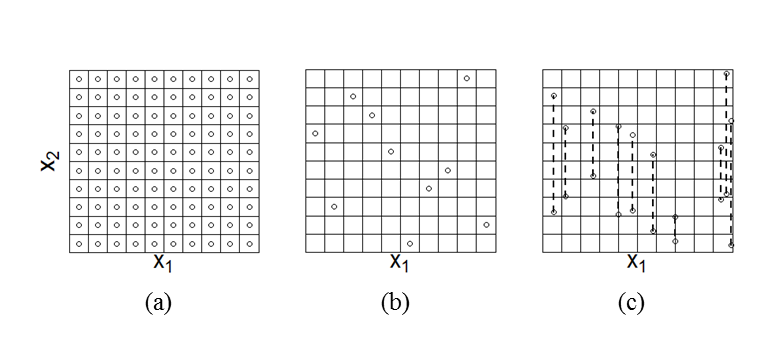
Figure C1. Different designs to sample from the parameter space. The full-factorial design (a) samples all combinations of a number of set values for each parameter (here we show only two parameters) and therefore allows for the computation of the sensitivity index for any of those parameters. The LHS design (b) samples only one value for each parameter. It does not allow for straightforward computation of the Sobol' indices, because Equation C1 asks for the computation of the expectation value of the model outcome while keeping one parameter fixed. In the full factorial design this would correspond to evaluation the sum of outcomes over a row or column, but in the LHS design we have only a single value per row or column and therefore cannot evaluate this sum. The design by Saltelli (2002) (c) samples pairs of points keeping one parameter fixed between each pair. The sensitivity index is estimated by the covariance between two vectors, each of which contains the model outcome that corresponds to one sample point out of every pair. The samples in the figure would allow for the computation of the sensitivity to \(x_1\). More points would have to be sampled to compute the sensitivity to \(x_2\). A simple test case illustrates the above discussion. We apply the sampling scheme to the model
$$ y=x_2+x_3. $$ (C7) With \(x_1,x_2,x_3 \sim U(0,1)\). The parameter \(x_1\) does not affect the outcome and thus \(S_{x1}=0\). The parameters \(x_2,x_3\) both affect the outcome equally and there are no interaction effects. Thus, \(S_{x2}= S_{x3}=0.5\). These values for the sensitivities are verified by analytic evaluation of Equation C3.
We apply the sampling design by Saltelli (2002) (Figure C1) for increasing sample size and compare the outcomes to the analytical values. Besides the sensitivities we also compare the outcomes for the total mean and variance. The relative deviations from the exact mean (i.e. the deviations from the exact mean as a percentage of the exact mean) are below 10% even for base sample sizes below 100 and below 2% for larger sample sizes (Figure C2). For the variance, the relative deviations from the exact value are below 10% for a sample size of the order \(10^3\) and are within a few percent for larger sample sizes (Figure C3). The sensitivity estimates, however, are less accurate (Figure C4). We encounter deviations from the exact values between 10–20% even for base sample sizes close to 5000. We cannot plot the relative deviation for \(S_{x1}\) because the analytic value is zero. The absolute estimates for the sensitivity reveal that the distribution is centred around the true value zero; The number of negative outcomes is approximately equal to the number of positive outcomes.
The example model of Equation C7 shows that even for a very simple test model, a large sample size is needed to accurately estimate sensitivities following the design by Saltelli (2002). This matches the finding that the sensitivity estimates for our ABM have wide confidence intervals (Figure 9). Furthermore, negative sensitivity estimates are not unlikely, especially for parameters that have little effect on the model outcomes. These negative estimates indicate the inaccuracy of the sampling design for estimating the sensitivities. We therefore suggest to report negative sensitivity estimates explicitly. For example, some of the sensitivity indices that we report in Figure 9 for our ABM test case have confidence intervals that are largely negative. Discarding these negative ranges by setting them to zero might give the reader an unrealistic confidence in the accuracy of the estimates.
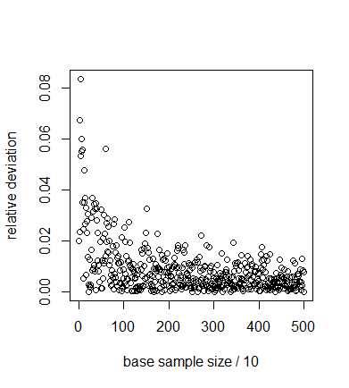
Figure C2. Relative absolute deviation of the estimate of the mean of the model outcomes from the true mean for increasing sample size. For large sample sizes, the estimate lies within 2% of the true value. 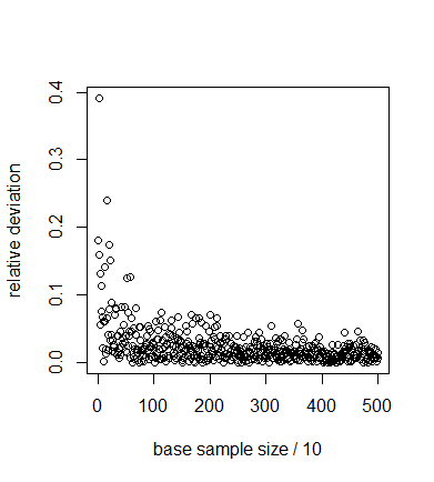
Figure C3. Relative absolute deviation of the estimate of the variance of the model outcomes from the true variance for increasing sample size. For large sample sizes, the estimate lies with a few percent of the true value. 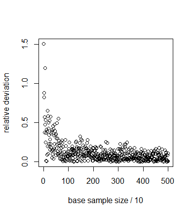
Figure C4. Relative deviation of the estimate of the sensitivity of x2 from the analytic value. Even for large sample sizes the deviations are significant. 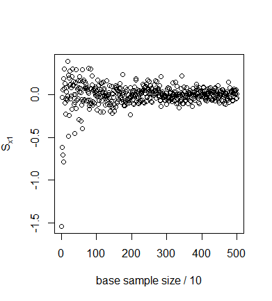
Figure C5. Estimate of the sensitivity to \(x_1\) for increasing sample size. The estimates are centred around the (correct) analytic value 0, but deviate significantly from this value.
References
- ARCHER, G.,
Saltelli, A.,
& Sobol', I. (1997). Sensitivity measures, ANOVA-like
techniques and the use of bootstrap. Journal of Statistical
Computation and Simulation, 58(2), 99–120. [doi:10.1080/00949659708811825]
AUDER, B., & Iooss, B. (2009). Global sensitivity analysis based on entropy. In Safety, reliability and risk analysis-Proceedings of the ESREL 2008 Conference (pp. 2107--2115). London: Taylor & Francis.
AXTELL, R. (1999). Why agents? on the varied motivations for agent computing in the social sciences. In Macal, C. M. & Sallach, D. (Eds.), Proceedings of the Workshop on Agent Simulation: Applications, Models, and Tools (pp. 3–24). Chicago: The University of Chicago Press.
BOUSQUET, F., & Le Page, C. (2004). Multi-agent simulations and ecosystem management: a review. Ecological modelling, 176(3), 313–332. [doi:10.1016/j.ecolmodel.2004.01.011]
BROWN, D. G., Page, S., Riolo, R., Zellner, M., & Rand, W. (2005). Path dependence and the validation of agent-based spatial models of land use. International Journal of Geographical Information Science, 19(2), 153–174. [doi:10.1080/13658810410001713399]
BURGERS, S. L., Hofstede, G. J., Jonker, C. M., & Verwaart, T. (2010). Sensitivity analysis of an agent-based model of culture's consequences for trade. In Progress in Artificial Economics (pp. 253–264). Springer Berlin Heidelberg. [doi:10.1007/978-3-642-13947-5_21]
CARIBONI, J., Gatelli, D., Liska, R., & Saltelli, A. (2007). The role of sensitivity analysis in ecological modelling. Ecological modelling, 203(1), 167–182. [doi:10.1016/j.ecolmodel.2005.10.045]
CROOKS, A., Castle, C., & Batty, M. (2008). Key challenges in agent-based modelling for geo-spatial simulation. Computers, Environment and Urban Systems, 32(6), 417–430. [doi:10.1016/j.compenvurbsys.2008.09.004]
CUKIER, R., Levine, H., & Shuler, K. (1978). Nonlinear sensitivity analysis of multiparameter model systems. Journal of computational physics, 26(1), 1–42. [doi:10.1016/0021-9991(78)90097-9]
DOWNING, D. J., Gardner, R. H., & Hoffman, F. O. (1985). An examination of response-surface methodologies for uncertainty analysis in assessment models. Technometrics, 27(2), 151–163.C [doi:10.1080/00401706.1985.10488032]
DRAPER, N. R., & Smith, H. (1998). Applied Regression Analysis , 3rd edition. John Wiley & Sons. [doi:10.1002/9781118625590]
FAGIOLO, G., Moneta, A., & Windrum, P. (2007). A critical guide to empirical validation of agent-based models in economics: Methodologies, procedures, and open problems. Computational Economics, 30(3), 195–226. [doi:10.1007/s10614-007-9104-4]
FICK, A. (1855). Ueber diffusion. Annalen der Physik, 170(1), 59–86. [doi:10.1002/andp.18551700105]
FILATOVA, T., Verburg, P. H., Parker, D. C., & Stannard, C. A. (2013). Spatial agent-based models for socio-ecological systems: challenges and prospects. Environmental Modelling & Software, 45, 1–7. [doi:10.1016/j.envsoft.2013.03.017]
GILBERT, N. (2002). Varieties of emergence. In D. Sallach (Ed.), Agent 2002: Social agents: ecology, exchange, and evolution (pp. 41–56). Chicago: University of Chicago and Argonne National Laboratory.
GILBERT, N. (2008). Agent-based models: Sage.
GRIMM, V., Berger, U., Bastiansen, F., Eliassen, S., Ginot, V., Giske, J., . . . Huse, G. (2006). A standard protocol for describing individual-based and agent-based models. Ecological modelling, 198(1), 115–126. [doi:10.1016/j.ecolmodel.2006.04.023]
GRIMM, V., Berger, U., DeAngelis, D. L., Polhill, J. G., Giske, J., & Railsback, S. F. (2010). The ODD protocol: a review and first update. Ecological modelling, 221(23), 2760–2768. [doi:10.1016/j.ecolmodel.2010.08.019]
HAMBY, D. (1994). A review of techniques for parameter sensitivity analysis of environmental models. Environmental monitoring and assessment, 32(2), 135–154. [doi:10.1007/BF00547132]
LEAMER, E. E. (1983). Let's take the con out of econometrics. The American Economic Review, 31–43.
LEAMER, E. E. (2010). Tantalus on the Road to Asymptopia. The Journal of Economic Perspectives, 31–46. [doi:10.1257/jep.24.2.31]
LIGMANN-ZIELINSKA, A., Kramer, D. B., Cheruvelil, K. S., & Soranno, P. A. (2014). Using Uncertainty and Sensitivity Analyses in Socioecological Agent-Based Models to Improve Their Analytical Performance and Policy Relevance. PloS one, 9(10), 235–247. [doi:10.1371/journal.pone.0109779]
LIU, H., Chen, W., & Sudjianto, A. (2006). Relative entropy based method for probabilistic sensitivity analysis in engineering design. Journal of Mechanical Design, 128(2), 326–336. [doi:10.1115/1.2159025]
LORSCHEID, I., Heine, B. O., & Meyer, M. (2012). Opening the 'black box'of simulations: increased transparency and effective communication through the systematic design of experiments. Computational and Mathematical Organization Theory, 18(1), 22–62. [doi:10.1007/s10588-011-9097-3]
MACAL, C. M., & North, M. J. (2010). Tutorial on agent-based modelling and simulation. Journal of Simulation, 4(3), 151–162. [doi:10.1057/jos.2010.3]
MATTHEWS, R. B., Gilbert, N. G., Roach, A., Polhill, J. G., & Gotts, N. M. (2007). Agent-based land-use models: a review of applications. Landscape Ecology, 22(10), 1447–1459. [doi:10.1007/s10980-007-9135-1]
PARKER, D. C., Manson, S. M., Janssen, M. A., Hoffmann, M. J., & Deadman, P. (2003). Multi-agent systems for the simulation of land-use and land-cover change: a review. Annals of the association of American Geographers, 93(2), 314–337. [doi:10.1111/1467-8306.9302004]
RAKOVEC, O., Hill, M. C., Clark, M. P., Weerts, A. H., Teuling, A. J., & Uijlenhoet, R. (2014). Distributed Evaluation of Local Sensitivity Analysis (DELSA), with application to hydrologic models. Water Resources Research, 50(1), 409–426. [doi:10.1002/2013WR014063]
SALTELLI, A. (2002). Making best use of model evaluations to compute sensitivity indices. Computer Physics Communications, 145(2), 280–297. [doi:10.1016/S0010-4655(02)00280-1]
SALTELLI, A., Ratto, M., Andres, T., Campolongo, F., Cariboni, J., Gatelli, D., Saisana, M., Tarantola, S. (2008). Global sensitivity analysis: The primer: John Wiley & Sons.
SALTELLI, A., Tarantola, S., Campolongo, F., & Ratto, M. (2004). Sensitivity analysis in practice: A guide to assessing scientific models: John Wiley & Sons.
SCHELLING, T. C. (1971). Dynamic models of segregation. Journal of mathematical sociology, 1(2), 143–186. [doi:10.1080/0022250X.1971.9989794]
SOBOL', I. M. (2001). Global sensitivity analysis indices for nonlinear mathematical models and their Monte Carlo estimates. Mathematics and Computers in Simulation, 55, 271–280. [doi:10.1016/S0378-4754(00)00270-6]
SWINSCOW, T. D. V. (1997). Statistics at square one. BMJ Publishing Group.
TARANTOLA, S., Gatelli, D., & Mara, T. A. (2006). Random balance designs for the estimation of first order global sensitivity indices. Reliability Engineering & System Safety, 91(6), 717–727. [doi:10.1016/j.ress.2005.06.003]
R CORE TEAM (2012). R: A language and environment for statistical computing.
THIELE, J. C., Kurth, W., & Grimm, V. (2014). Facilitating Parameter Estimation and Sensitivity Analysis of Agent-Based Models: A Cookbook Using NetLogo and 'R'. Journal of Artificial Societies and Social Simulation, 17(3). [doi:10.18564/jasss.2503]
WILENSKY, U. 1999. NetLogo. http://ccl.northwestern.edu/netlogo/. Center for Connected Learning and Computer-Based Modeling, Northwestern University. Evanston, IL.
WINDRUM, P., Fagiolo, G., & Moneta, A. (2007). Empirical validation of agent-based models: Alternatives and prospects. Journal of Artificial Societies and Social Simulation, 10(2), 8.