On the Interplay Among Multiple Factors: Effects of Factor Configuration in a Proof-Of-Concept Migration Agent-Based Model

, ,
and
aPrinceton University, United States; bUniversity of Florida, United States
Journal of Artificial
Societies and Social Simulation 25 (2) 7
<https://www.jasss.org/25/2/7.html>
DOI: 10.18564/jasss.4793
Received: 24-Jul-2021 Accepted: 14-Mar-2022 Published: 31-Mar-2022
Abstract
Many researchers have addressed what factors should be included in their models of coupled natural-human systems (CNHSs). However, few studies have explored how these factors should be incorporated (factor configuration). Theoretical underpinning of the factor configuration may lead to a better understanding of systematic patterns and sustainable CNHS management. In particular, we ask: (1) can factor configuration explain CNHS behaviors based on its theoretical implications? and (2) when disturbed by shocks, do CNHSs respond differently under varying factor configurations? A proof-of-concept migration agent-based model (ABM) was developed and used as a platform to investigate the effects of factor configuration on system dynamics and outcomes. Here, two factors, social ties and water availability, were assumed to have alternative substitutable, complementary, or adaptable relationships in influencing migration decisions. We analyzed how populations are distributed over different regions along a water availability gradient and how regions are culturally mixed under different factor configurations. We also subjected the system to a shock scenario of dropping 50% of water availability in one region. We found that substitutability acted as a bu er against the effect of water deficiency and prevented cultural mixing of the population by keeping residents in their home regions and slowing down residential responses against the shock. Complementarity led to the sensitive migration behavior of residents, accelerating regional migration and cultural mixing. Adaptability caused residents to stay longer in new regions, which gradually led to a well-mixed cultural condition. All together, substitutability, complementarity, and adaptability gave rise to different emergent patterns. Our findings highlight the importance of how, not just what, factors are included in a CNHS ABM, a lesson that is particularly applicable to models of interdisciplinary problems where factors of diverse nature must be incorporated.Introduction
Recent studies of coupled natural-human systems (CNHSs) have drawn much attention to interplays between social and natural factors in a wide variety of situations (Liu et al. 2007). Many scholars have focused on "what" factors should be included in CNHS models (An 2012; Liu et al. 2007), but the question of "how" these factors should be incorporated has largely been overlooked; herein, we will refer to how factors are incorporated as "factor conFiguretion." This issue was recently raised by CNHS researchers (Boas et al. 2019; Kramer et al. 2017; Metson et al. 2015; Morzillo et al. 2015). What if factor conFiguretion itself is more significant to outputs than the mere inclusions of these factors? Factor conFiguretion may even build unique patterns, e.g., flickering patterns, yet existing studies were restricted to examining this aspect. Factor conFiguretion reflects a theoretical implication on how the factors interact and thus leads to a better understanding of decision-making processes for CNHSs.
Agent-based models (ABMs) take a bottom-up CNHS modeling approach that captures how individuals make their own decisions, follow different rules, and interact with each other in heterogeneous environments (Farmer & Foley 2009; Grimm et al. 2005). ABMs’ strengths make them a great modeling tool to study the effect of factor conFiguretion. First, ABMs are capable of simultaneously handling both natural and social factors (Bell et al. 2019; Bousquet & Le Page 2004; Loomis et al. 2008). Second, ABMs allow us to include factor conFiguretion into an individual’s decision-making processes and generate system-level patterns (An 2012; Gimblett 2002). Third, we can test different shock scenarios and capture emergent CNHS responses against shocks (Waldrop 2018).
The objective of this study is to explore the effects of factor conFiguretion on system dynamics and outcomes of a simple CNHS ABM. To provide the context and narrative for interpreting the results, we use a highly simplified ABM of migration processes. It is important to note here that the simplified migration ABM is used as a platform for investigating the effects of factor conFiguretion and is not meant to capture all the complexity of migration process. Indeed, migration is a complex CNHS process, involving a large array of natural and social drivers interacting at multiple temporal and spatial scales and producing multi-dimensional outcomes (Abel et al. 2019; Adger et al. 2014; Black et al. 2011; Czaika & De Haas 2014). Within the context of this simple ABM, we first delved into how different conFiguretions of multiple factors influence individual-level decisions and systematic patterns. We especially looked into the flickering-like behavior—agents in two regions collectively switch their locations back and forth—in a certain conFiguretion (in Figures 5c and 5d). This study then tested the effect of factor conFiguretions in a shock scenario. We considered both stationary values and time series of system outcomes after the shock for this analysis.
Methods
A proof-of-concept migration ABM
In this study, a simple, proof-of-concept migration ABM is used as a platform to investigate the effects of factor conFiguretion on system dynamics and outcomes. Our ABM incorporates a two-staged migration decision-making process (Champion et al. 2003; Rees et al. 2006; Stillwell 2005), focusing on a few key drivers of migration, namely distance, social ties, and the environment (e.g., water availability). We included water availability differences as a natural factor, based on migration case studies caused by water scarcity (Jägerskog et al. 2016) and previous examples of ABMs of migration (Krol & Bronstert 2007; Magallanes et al. 2014; Rigaud et al. 2018; Smajgl et al. 2015). The second factor was cultural affinitysocial ties connecting people from the same home region. Social network ties are essential in migration modeling as they are closely related to migration decisions (Klabunde & Willekens 2016), e.g., information transmission through social connections pulls more people with the same culture to the ethnic enclaves. Lastly, we also used region-to-region distance as a physical factor because the effect of distance is evident in choosing a destination to migrate (Ravenstein 1885; Schwartz 1973).
Model structure
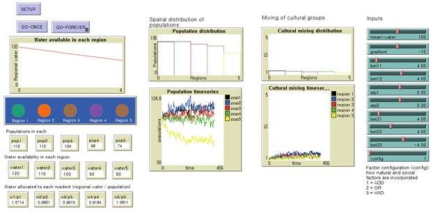
In the model, five regions are placed at regular intervals along a vector (Figure 1). Each region is assumed to have a different total water availability (\(w_i\) at Region \(i\)) that is constant over time, though per capita water availability changes with the population (\(w_i/n_i\) at Region \(i\), where \(n_i\) is the population at Region \(i\)). Water availability of the five regions linearly decreased from left to right (imagine a river or a lake to the left of these five regions), based on the following relationship, \(w_i=s(i-3)+m\), where \(s\) represents the water availability gradient and \(m\) the average water availability across the five regions. Initially, 100 residents lived in each region and considered it their "homeland." When people in Region \(i\) decide to choose a migration destination, they consider the number of people from their homeland in potential destination, Region \(j\) (\(n_{i,j}\)), as a beneficial factor (e.g., cultural enclave).
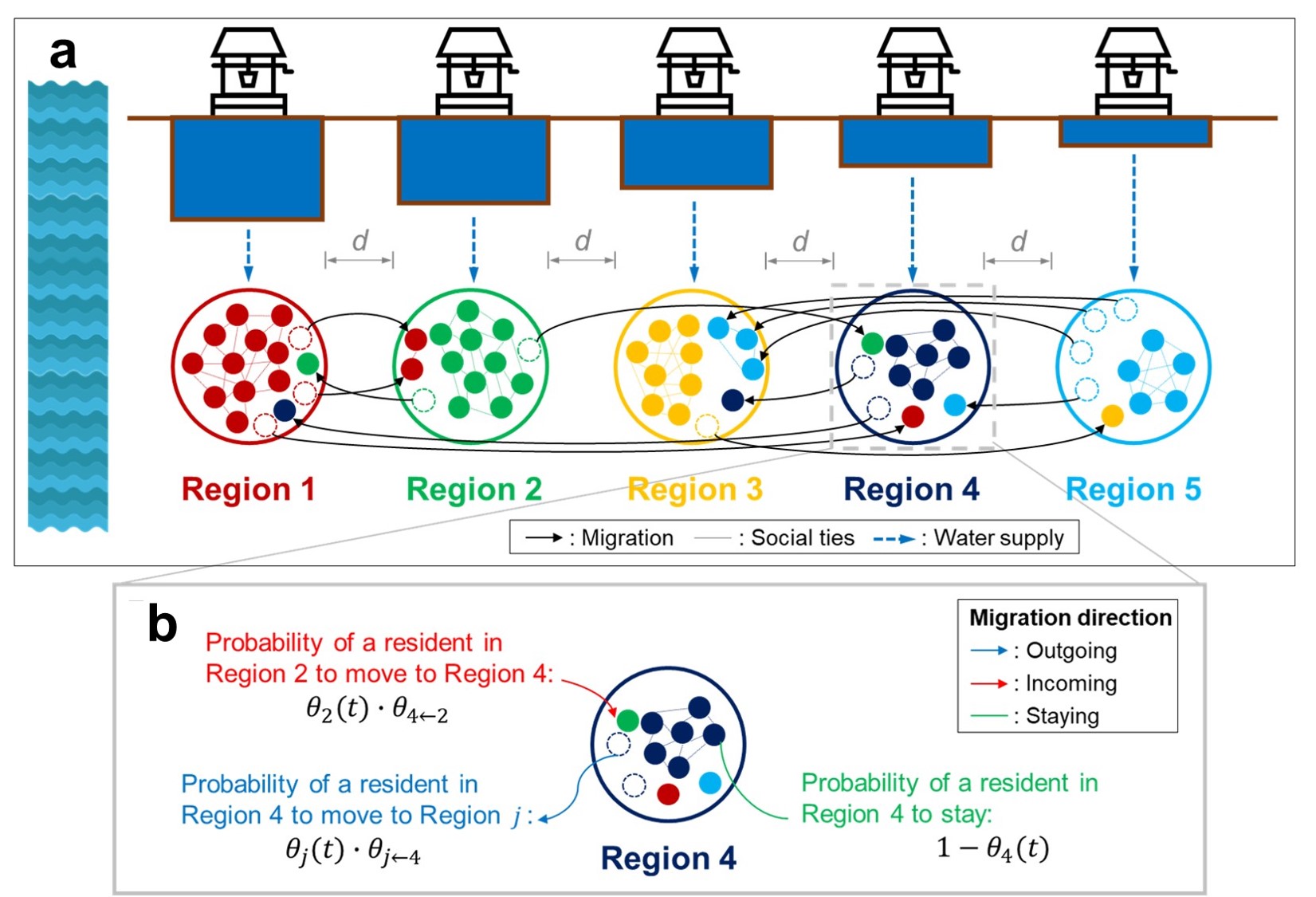
In this model, the decision-making process of a resident is divided into two stages. In the first stage, a resident (small circle in Figure 1a) decides whether to stay or to leave. Low water availability and/or weak social ties "push" people from the current region, while an aggregate effect of the two factors is dependent on the factor conFiguretion. In the second stage ("pull"), he/she chooses which region to migrate to. The residents then consider the destination’s water availability and stronger social ties as well as the distance from their current region; as in the first stage, the total "pull" effect depends on the factor conFiguretion. Residents in each region equally share the water available in that region at every time step and make decisions according to their social and environmental conditions. Each resident has a probability of staying \(\mu_o (t)\) (\(o=\) origin) (first-stage decision). For those who decide to leave, they have a probability \(\theta_{j\leftarrow{}o} (t)\) (\(j=\) destination) to go to Region \(j\) (second stage decision). Social ties and water allocated to a person affect both stages, while distance is only considered in the second stage. Depending on the type of factor conFiguretion described in the next section, the migration probabilities of the two stages take different forms. An ODD protocol (Grimm et al. 2010) of the ABM provides a more detailed explanation in Appendix C. The model code can be found at: https://www.comses.net/codebase-release/43c48c8c-a654-4c64-94ef-f6a477c08702/.
Factor conFiguretion
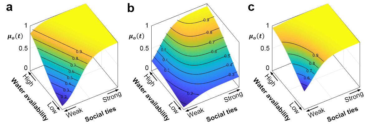
Three possible conFiguretions between natural and social factors are explored: ADD, AND, and OR (Figure 2 and Table 1).
Substitutable factor conFiguretion (ADD) linearly combines the two factors, following the constant elasticity of substitution (CES) production function in neoclassical economics (e.g., Fenichel & Zhao 2015; Markandya & Pedroso-Galinato 2007). The relation between factors can be compared to drinking soda products. You could drink, for example, one of two alternative brands (factors). If one is insufficient, another can be an alternative. The two factors have the same functionality so that one can substitute for the other. Despite this rather strong implicit assumption of substitutability among factors, this conFiguretion is the most widely used in many migration models (e.g., An et al. 2020; Cai & Oppenheimer 2013; Li et al. 2020).
| ConFiguretion | Equation | |
|---|---|---|
| \(F_1 =\) | ADD | \(\mu_o (t)=\frac{e^{\beta_1^{(1)}\left(x^{(1)}-\alpha^{(1)}\right)+\beta_1^{(2)}\left(x^{(2)}-\alpha^{(2)}\right)}}{1+e^{\beta_1^{(1)}\left(x^{(1)}-\alpha^{(1)}\right)+\beta_1^{(2)}\left(x^{(2)}-\alpha^{(2)}\right)}}\) |
| AND | \(\mu_o (t)=\left(\frac{e^{\beta_1^{(1)}\left(x^{(1)}-\alpha^{(1)}\right)}}{1+e^{\beta_1^{(1)}\left(x^{(1)}-\alpha^{(1)}\right)}}\right) \left(\frac{e^{\beta_1^{(2)}\left(x^{(2)}-\alpha^{(2)}\right)}}{1+e^{\beta_1^{(2)}\left(x^{(2)}-\alpha^{(2)}\right)}}\right) \\= \frac{e^{\beta_1^{(1)}\left(x^{(1)}-\alpha^{(1)}\right)+\beta_1^{(2)}\left(x^{(2)}-\alpha^{(2)}\right)}}{1+e^{\beta_1^{(1)}\left(x^{(1)}-\alpha^{(1)}\right)+\beta_1^{(2)}\left(x^{(2)}-\alpha^{(2)}\right)}+e^{\beta_1^{(1)}\left(x^{(1)}-\alpha^{(1)}\right)}+e^{\beta_1^{(2)}\left(x^{(2)}-\alpha^{(2)}\right)}}\) | |
| OR | \(\mu_o (t)=1-\left(\frac{1}{1+e^{\beta_1^{(1)}\left(x^{(1)}-\alpha^{(1)}\right)}}\right) \left(\frac{1}{1+e^{\beta_1^{(2)}\left(x^{(2)}-\alpha^{(2)}\right)}}\right) \\ = \frac{e^{\beta_1^{(1)}\left(x^{(1)}-\alpha^{(1)}\right)+\beta_1^{(2)}\left(x^{(2)}-\alpha^{(2)}\right)}+e^{\beta_1^{(1)}\left(x^{(1)}-\alpha^{(1)}\right)}+e^{\beta_1^{(2)}\left(x^{(2)}-\alpha^{(2)}\right)}}{1+e^{\beta_1^{(1)}\left(x^{(1)}-\alpha^{(1)}\right)+\beta_1^{(2)}\left(x^{(2)}-\alpha^{(2)}\right)}+e^{\beta_1^{(1)}\left(x^{(1)}-\alpha^{(1)}\right)}+e^{\beta_1^{(2)}\left(x^{(2)}-\alpha^{(2)}\right)}}\) | |
| \(F_2 =\) | ADD | \(\theta_{j\leftarrow{}o} (t)=C_{ADD}\frac{e^{\beta_2^{(1)}\Delta x_{jo}^{(1)}+\beta_2^{(2)} \Delta x_{jo}^{(2)}}}{1+e^{\beta_2^{(1)}\Delta x_{jo}^{(1)}+\beta_2^{(2)} \Delta x_{jo}^{(2)}}} / e^{\beta_2^{(3)} \Delta x_{jo}^{(3)}}\) |
| AND | \(\theta_{j\leftarrow{}o} (t)=C_{AND}\left(\frac{e^{\beta_2^{(1)}\Delta x_{jo}^{(1)}}}{1+e^{\beta_2^{(1)}\Delta x_{jo}^{(1)}}}\right) \left(\frac{e^{\beta_2^{(2)}\Delta x_{jo}^{(2)}}}{1+e^{\beta_2^{(2)}\Delta x_{jo}^{(2)}}}\right) / e^{\beta_2^{(3)} \Delta x_{jo}^{(3)}}\) | |
| OR | \(\theta_{j\leftarrow{}o} (t)=C_{OR}\left\{1-\left(\frac{1}{1+e^{\beta_2^{(1)}\Delta x_{jo}^{(1)}}}\right) \left(\frac{1}{1+e^{\beta_2^{(2)}\Delta x_{jo}^{(2)}}}\right)\right\} / e^{\beta_2^{(3)} \Delta x_{jo}^{(3)}}\) | |
In the complementary factors conFiguretion (AND), the two factors are complementary. For example, both soil moisture and solar radiation are needed for a plant to grow. If either one is insufficient, the plant will wither and die. This case requires both factors for an event to occur. In our model, a resident will stay in the current location (first-stage decision) when the water availability is high and social ties are strong; otherwise, the resident is likely to migrate to other regions. Similarly, in the second stage, the resident prefers a destination with high water availability and strong social ties.
In the adaptable factors conFiguretion (OR), one factor alone can be enough for an event to happen. For example, on a domestic flight, you may bring either a driver’s license or a passport as a form of identification. In our model, this means that a resident is likely to stay when either high water availability or strong social ties. For those who leave, they prefer a destination with either high water availability or strong social ties.
As discussed in previous paragraphs, different factor conFiguretions reflect different theoretical reasoning. Our work offers novel insights into the rules of interactions among multiple factors and their implications in a simple ABM. These lessons can further be extended to other CNHS models. It is also worth noting that the mathematical formulations of the factor conFiguretion capture nonlinear interactions between the factors without the "product" terms (e.g., \(\beta^{(1,2)} x^{(1)} x^{(2)}\)), used in most models that aim to capture nonlinear interactions.
We explored some parameter values and in our companion paper (Carmona-Cabrero et al., under preparation), also conducted global sensitivity analysis to determine the importance of the factor conFiguretion on the system outcomes compared to the specific values used for the input parameters. We found that factor conFiguretion had an influential effect (i.e., explains > 90% of the outputs variance) on population distributions except for the population in Region 3, where stochasticity was critical to the outcome.
Systematic patterns: Spatial distribution of population and cultural diversity
To investigate the effects of factor conFiguretion, we considered two systematic patterns of populations: Spatial distributions of population and the mixing of cultural groups. We ran 75 ABM realizations under each factor conFiguretion. Selecting the appropriate number of realizations (\(N=75\)) is addressed in Appendix A.
Initially, each region has 100 residents. Then, regional populations are counted after the system reaches stable dynamics to understand how populations are distributed over five regions. The level of cultural mixing or diversity is also an important social character of a population, influencing population movements in complex ways (Jiang et al. 2010; Nathan 2011). Here, Simpson’s index from biodiversity literature (Quétier et al. 2007; Simpson 1949) is used to quantify how well cultural groups are mixed in Region \(j\). Previous sociological studies have applied Simpson’s index in the context of social diversity (Blau 1977; Rushton 2008), and the U.S. Census Bureau has used it to explain degrees of ethnic diversity in the U.S. (U.S. Census Bureau 2021). This index identifies whether a region is dominated by one cultural group or well-mixed with several groups—such cultural diversity may attract some people or cause social tension; although these consequences and feedbacks have not been explicitly incorporated in this present model yet, we believe that it is important to determine how diversity is affected by the factor conFiguretion. We used an inverse form of Simpson’s index for an easier interpretation:
| \[ D_j=\frac{1}{\sum_{i=1}^5 \left(p_i^j \right)^2},\] | \[(1)\] |
We also explored population responses after a disturbance in the CNHS, namely what would happen to the spatial distributions of population and mixing of cultural groups when water supply in Region 1 reduced to 50% by an unexpected shock?
Results and Discussion
Spatial distributions of population and mixing of cultural groups
We first considered patterns under the pre-shock condition. When the factor conFiguretion was ADD, populations were distributed in a quadratic-like form from Regions 1-5, peaking at Region 2 and dropping at Region 5 (blue boxplots in Figure 3a); Region 1 had slightly fewer residents, and the population decreased from Region 2 to Region 5. In water-rich regions (Regions 1 and 2), high water availability and strong social ties kept locals in (high \(\mu_o (t)\) in Figures 7a and 7b of Appendix B). These regions accommodated more "foreigners" from other regions because weak social ties could be substituted by high water availability. However, foreigners were likely to return to their homelands because when many of these foreigners moved into water-rich regions, their per capita water availability reduced and could no longer substitute weak social ties. In the water-poor region, i.e., Region 5, low water availability cannot make up for weak social ties, so foreigners avoid the region. Comparing with other regions, Region 5’s locals also tended to out-migrate more due to low water availability, leading to the lowest population in Region 5. Region 1 was less populated than Region 2, despite its higher water availability. Here, distance played an important role in deciding which region to move to in the second-stage decision. Residents in water-poor regions were more likely to migrate to Region 2 simply because Region 2 was closer. Under the ADD conFiguretion, regions were relatively culturally segregated (low values of \(D_j\); blue boxplots in Figure 3d), with water-rich regions being more culturally mixed. High water availability can substitute for weak social ties of foreigners so that these regions could attract more foreigners.
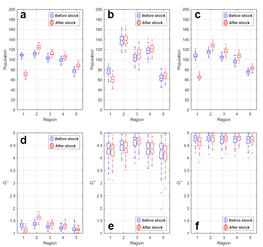
A similar trend was observed with a more pronounced gradient in the OR conFiguretion (blue boxplots in Figure 3c). In this case, either one factor alone was enough to keep a resident. That is, residents were "more tolerant" to changes in either social ties or water availability. It turned out that this adaptability diluted the effects of social ties, leading to more culturally well-mixed conditions (blue boxplots in Figure 3f). With greater diversity, all regions had similar strengths of social ties. Residents’ decisions now became more dependent on water availability relative to other conFiguretions; more people migrate from water-poor to water-rich regions. Note that the more pronounced distribution of populations implies greater equality in per capita water availability.
Under the AND factor conFiguretion, spatial distributions of the population had more irregular patterns than ADD and OR conFiguretions (blue boxplots in Figure 3b). Under this conFiguretion, natural and social factors are complementary: A resident needs both to stay. The results suggested that residents were sensitive to changes in either water availability or social ties, showing highly mobile behaviors. Highly mobile and uncertain characters of residents led to irregular population distributions. Also, all regions became culturally well-mixed conditions and weakened social ties (blue boxplots in Figure 3e).
Spatial distributions of population and mixing of cultural groups after shocks
In response to a shock of water availability (50% reduction) in Region 1, residents in Region 1 out-migrated to other regions (red boxplots in Figure 3). Median populations in Region 1 reduced to similar amounts (70 and 65) after the shock in ADD and OR conFiguretions (red boxplots in Figures 3a and 3c), yet post-shock transition forms were different between the two (Figrues 4a and 4c). Populations in the disturbed region gradually decreased in the ADD conFiguretion. Substitutability absorbed shocks on water availability, preventing a sudden population decrease (Figure 4a). Moreover, residents in Region 1 moved to other regions at different rates. Out-migrating residents in Region 1 were mostly locals under the ADD conFiguretion. As in the pre-shock case, the distance factor was the most critical in choosing which region to move. Thus, the closer a region was to Region 1, the faster new migrants moved to the region.
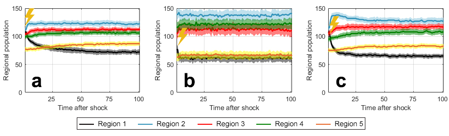
Populations in Region 1 dropped more sharply in the OR conFiguretion (Figure 4c): Residents had weaker social ties (because it is culturally mixed; Figure 3f) so that a shock in water availability more strongly affected population movements. Most of these residents transit Region 2 and then spread to other regions (the population in Region 2 rapidly increases, reaches a peak, and gradually decreases in Figure 4c). This behavior appeared inconsistent with the OR conFiguretion’s characteristic of being more tolerant, as discussed in the previous section. This seeming inconsistency came from different strengths of social ties in ADD and OR conFiguretions. In the ADD conFiguretion, each region became dominated by locals who had strong social ties (Figure 3d). Regions were culturally mixed in the OR conFiguretion, and residents had weaker social ties. The strength of "pull" became weaker given that regions before the shock were culturally well-mixed, and social ties were not important anymore.
In the AND conFiguretion, populations in the disturbed region did not change greatly like the other two cases (Figures 3b and 4b). Populations in Region 1 were already low under the AND conFiguretion before the shock. This result indicates that per capita water availability was relatively high. Thus, Region 1 was less influenced by the shock than in other conFiguretions. Residents still abruptly out-migrated from Region 1 right after the shock. It is because staying probability (\(\mu_o(t)\)) drops immediately to deficiency in any one of the factors under the AND conFiguretion (see how \(\mu_o(t)\) changes according to one factor when another factor is sufficient in Figure 2b). This behavior reflects AND’s sensitive nature.
The mixing of cultural groups after the shock varied across factor conFiguretions. AND and OR conFiguretions did not exhibit significant changes in cultural diversity after the shock (Figures 3e and 3f). Both locals and foreigners in Region 1 had weak social ties before the shock due to the culturally well-mixed condition in these conFiguretions. After the shock, Region 1 residents suffered from low water availability and weak social ties. No matter which cultural group a resident belonged to, he/she moved out of the region. Cultural diversity was maintained at similar levels. ADD conFiguretion exhibited more significant changes in cultural mixing in the shock scenario. When Region 1 was disturbed, both locals and foreigners out-migrated (population movements of locals were much greater). Foreigners could previously stay in Region 1 as high water availability replaced weak cultural affinity. Now that Region 1 could not make up for weak cultural affinity, most of the foreigners in Region 1 moved to other regions, leading to the almost homogeneous cultural condition (\(D_j \approx 1\)). Out-migration from Region 1 increased cultural diversity in other close regions (red boxplots in Figure 3d).
Our model results highlighted the importance of how factors are put together in a model. In the context of this proof-of-concept ABM, how agents took water availability and social ties into accountthat is, how they configured these two factorsled to differences in resulting population patterns and aftershock responses. Many of these different patterns and changes could be explained by the types of relationships between the two factors encapsulated by our three factor conFiguretions, namely substitutability (ADD), complementarity (AND), and adaptability (OR). When one of the factors became unfavorable at the origin, substitutability provided some buffer to soften the effects, complementarity led agents to become quite sensitive and incentivized to leave, and adaptability enabled people to stay longer in a new environment after they migrated.
Factor conFiguretions were useful, but using them to differentiate underlying mechanisms of population movements was not always straightforward. For example, the population transition in Region 1 after the shock was not more tolerant in the OR conFiguretion than in the ADD conFiguretion (Figure 4c). Underlying mechanisms fit well into the theoretical implications of factor conFiguretion if all factors are at similar levels. Nonetheless, factor conFiguretion still offered a way for us to interpret some of these different situations in a coherent way.
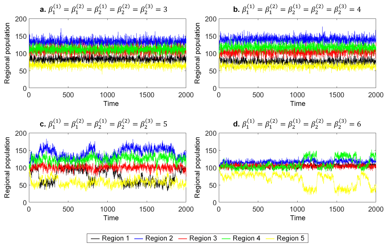
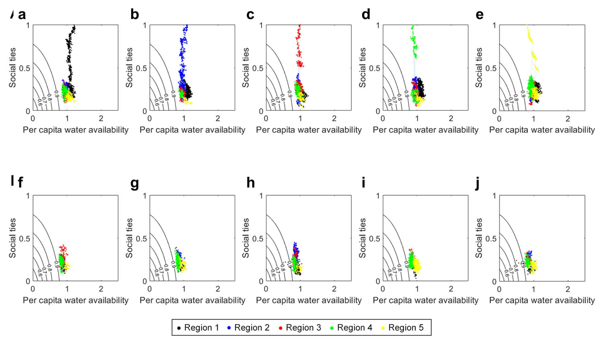
Although the population time series reached stationary ranges in the current parameter set, this is not always the case. With larger \(\beta\) values (\(\beta_1^{(1)}=\beta_1^{(2)}=\beta_2^{(1)}=\beta_2^{(2)}=\beta_2^{(3)}=5\) or \(6\)) and \(\alpha^{(1)}=\alpha^{(2)}=0.3\) under the AND conFiguretion, some populations alternated back-and-forth between low and high values (Figures 5c and 5d), akin to the so-called "flickering" of a bistable dynamical system approaching a regime shift (Dakos et al. 2013; Scheffer et al. 2009; Taylor et al. 1993; Wang et al. 2012). The back-and-forth movement was caused by collective movement and return between neighboring regions (Regions 1 and 2 in Figure 5c or Regions 4 and 5 in Figure 5d). Interestingly, such back-and-forth migration patterns have been documented in some migration cases of the real world, e.g., short-term migration in India (Bala 2017), camps of displaced citizens in Haiti (Fondation Scelles 2014). Transnationalism literature also discussed back and forth migrations between two locations (Adams & Kasakoff 2004; White 2012). This simple model was rich enough to exhibit diverse patterns according to the changes in \(\beta\) values. \(\beta\) parameters did affect the model outcomes, yet factor conFiguretion more critically controlled the outcomes, proven by our companion paper (Carmona-Cabrero et al., under preparation). To be clear, the flickering-like behavior was only observed when \(\beta\) values were large in the AND conFiguretion, but not in other cases.
Conclusions
This study used a proof-of-concept ABM in a stylized migration problem to answer the following research questions: (1) how does factor conFiguretion between social and natural factors affect systematic patterns? and (2) how are post-shock responses distinguished by the factor conFiguretion? In this particular ABM, factor conFiguretion reflected the interactions between cultural affinity and water availability in influencing an agent’s decisions. Our results suggested that spatial distributions of the population and the mixing of cultural groups can differ significantly according to the factor conFiguretion. Substitutability, complementarity, and adaptability (ADD, AND, and OR conFiguretions, respectively) exhibited different spatial distributions of population and cultural mixing. In the ADD conFiguretion, substitutability resulted in quadratic spatial distributions of population and cultural segregation. High mobility and uncertainty of complementarity shaped irregular population distributions and culturally well-mixed conditions in the AND conFiguretion. Adaptability showed linear population distributions proportional to water availability and high cultural diversity in the OR conFiguretion. Furthermore, we observed nonlinear responses in emergent patterns, both population distribution and cultural mixing, under different factor conFiguretions in a shock scenario. ADD and OR conFiguretions exhibited great population changes in Region 1, while the change was more abrupt in the OR case. AND and OR conFiguretions maintained culturally well-mixed conditions to similar levels after the shock. On the other hand, ADD conFiguretion had different post-shock responses. Region 1 became almost culturally unmixed, and Regions 2-5 increased their degrees of cultural mixing. These aftershock population patterns were sometimes unexpected because social and natural factor conditions were different for all conFiguretions right before the shock. Population transitions, population distributions, and cultural mixing after the shock could still be explained through theoretical implications of factor conFiguretion considering these differences. In sum, these results highlight the importance of how, not just what, natural and social factors are incorporated into ABMs.
In this paper, we aimed to highlight the effect of factor conFiguretion rather than to build a realistic model of any particular system. We are aware that real-world migration involves other drivers related to politics, demographics, and economics (Black et al. 2011). Incorporating all these drivers in the model, however, would have hindered us in answering our research questions in a clear fashion. Thus, our ABM was purposefully built upon a minimalistic design in the conceptual environment. We reduced migration decision-making dimensions by selecting cultural affinity (social factor) and water availability (natural factor) as drivers. Such a design facilitated us to understand the primary mechanisms of the problemthe effect of factor conFiguretion. Our future work includes implementing several factor conFiguretions to real-world cases and verifying applicability in more complex models, using the present model as a benchmark to capture missing migration factors (e.g., disaster, fatality, income, etc.) at different stages.
While our focus here is on how different factors are configured in an ABM, ABMs of such complex processes as migration have other challenges: They tend to involve many parameters to codify the many rules that govern their agents, so many that sometimes it is difficult to tell which parameters and their interactions drive the model outcomes. Our ongoing work addresses that challenge by conducting global sensitivity and uncertainty analysis on the model to disentangle the direct and interactive effects of the model’s inputs (Carmona-Cabrero et al., under preparation). This helps to inform management of the system and to evaluate the model.
Our lessons and findings about the importance of how, not just what, factors are included in an ABM are applicable to other models of co-evolutionary systems, including CNHS, socio-ecological systems, and socio-technical systems. These models integrate several componentse.g., humans, ecology, hydrology, technology, infrastructure, etc.and therefore require an understanding of how components are incorporated. Clarifying the effects of the way in which multiple factors are configured will improve the development of these complex models as well as their contributions to the development of a coherent theory.
Acknowledgements
The research reported here was supported by the Army Research Office/Army Research Laboratory under award #W911NF1810267 (Multidisciplinary University Research Initiative). The views and conclusions contained in this document are those of the authors and should not be interpreted as representing the official policies either expressed or implied of the Army Research Office or the U.S. Government. Woi Sok Oh is also pleased to acknowledge the support of the Princeton University Dean for Research, High Meadows Environmental Institute, and Andlinger Center for Energy and the Environment at Princeton University.Appendix
Appendix A: Selection of the Number of ABM Realizations
Since this model is stochastic, we need to run the model several realizations with the same inputs for robust results. The realization size should be large enough to make outputs representative and robust for the same inputs by reducing the the effect of stochasticity over the outputs. At the same time, it should be computationally efficient without excessive runs to minimize the simulation duration. We used bootstrapping technique to identify the best realization size objectively in this tradeoff.
We bootstrapped two outputs at 2000 time step (pre-shock condition) in the AND conFiguretion: the population in Region 3 and the degree of cultural mixing in Region 3 (\(D_3\)) in the AND conFiguretion. AND conFiguretion was the most variable and uncertain from our understanding. The realization size selected from the AND conFiguretion would produce stable outputs in the other two conFiguretions. Also, Region 3 was particularly the most stochastic among the five regions as it often worked as a transit. Therefore, the optimal realization size selected from these outputs will be used for other outputs and factor conFiguretions.
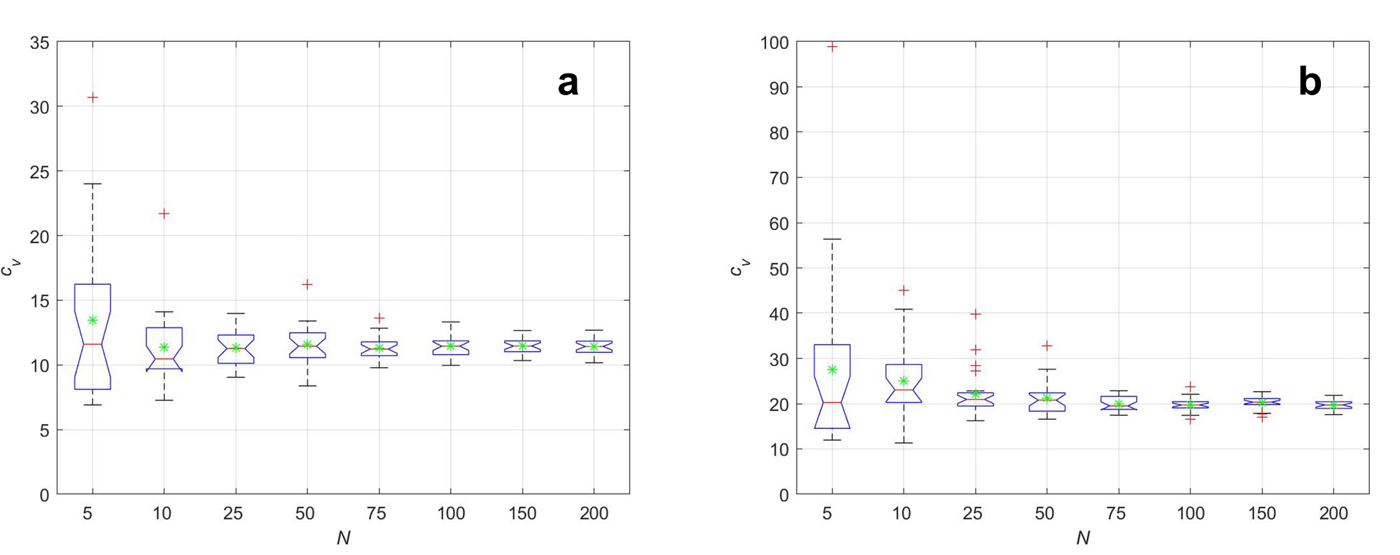
First, the model generated results for 200 iterations with the same inputs. We then resampled \(N\) outputs from 200 realizations. Here, \(N\) is directly related to the realization size. We tested different resampling sizes of \(N=5,10,25,50,75,100,150,200\). Coefficient of variation was calculated with \(N\) resampled outputs:
| \[c_v=\mu_s/\sigma_s ,\] | \[(2)\] |
where \(\mu_s\) is the mean of \(N\) resampled outputs, and \(\sigma_s\) is the standard deviation of \(N\) resampled outputs. \(c_v\) involves the relative variability of \(N\) resampled outputs. Resampling and \(c_v\) calculation were repeated 25 times for each \(N\).
Figure 6 presents distributions of \(c_v\) in different N values. When comparing mean, median, and range between minimum and maximum scores, statistical properties converged to the values of large \(N\) results from \(N=50-75\). Thus, we selected \(N=75\) for more stable results in the model analysis.
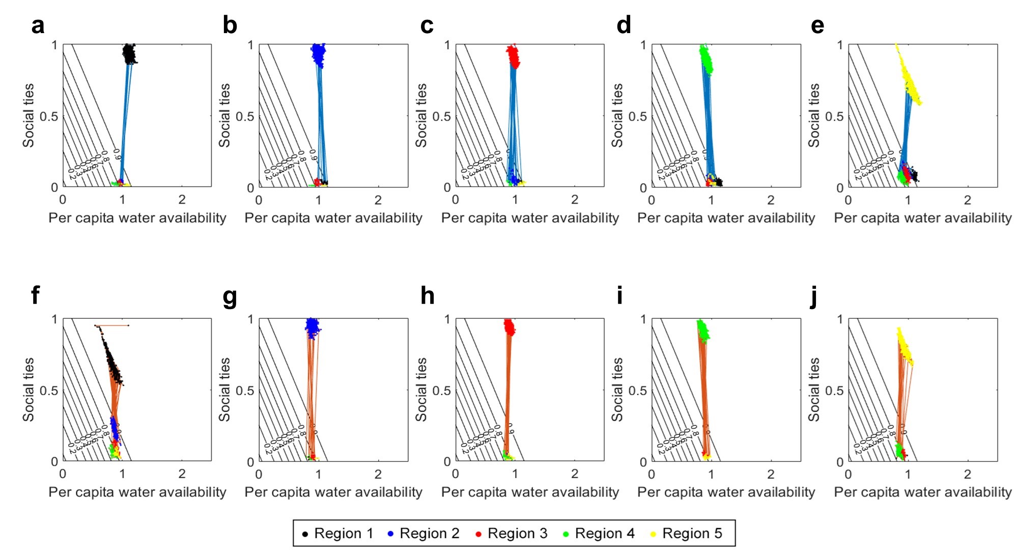
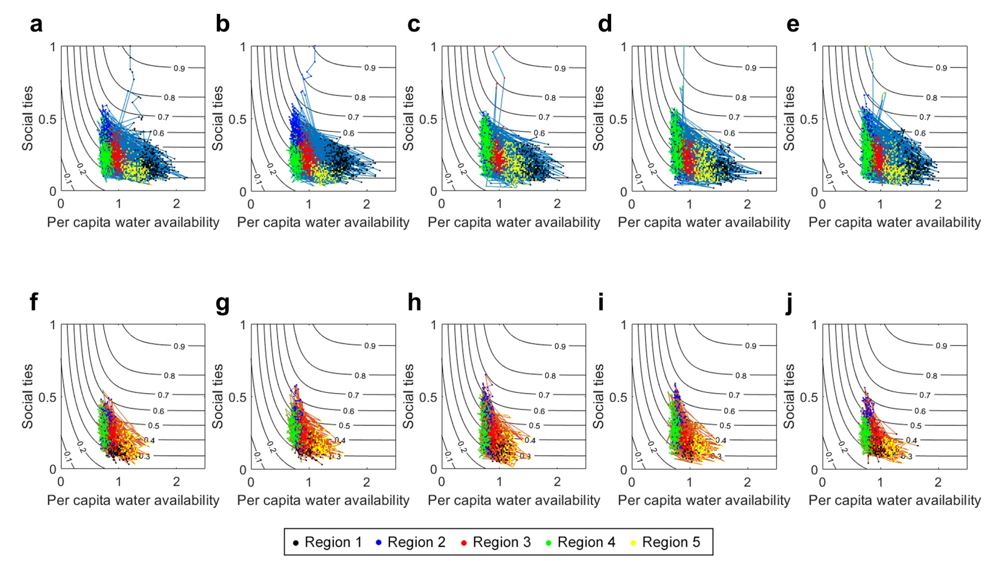
Appendix B: Trajectories of Per Capita Water Availability, Social ties, and Staying Probability Under Different Factor ConFiguretions
Appendix C: ODD Protocol
Overview
This ODD (Overview, Design concepts, and Details) protocol provides detailed information of our ABM that is not explained in the main text of the manuscript.
Purpose
This model is built upon a proof-of-concept condition to verify the effects of factor conFiguretion in simplified migration decision-making processes. The model particularly focuses on incorporating cultural affinity as a social factor and water availability per resident as a natural factor. The model aims to (i) reveal how different factor conFiguretions influence the emergent patterns and (ii) explore how factor conFiguretions are related to changing regimes of system outcomes in response to unexpected shock.
Entities, state variables, and scales
The environment of this stylized model is five patches in a row (in the x-axis direction), representing five independent regions (Figures 1 and 10). Neighboring regions are one patch away from each other. Available water in Region \(j\) (\(w^j\)) is linearly decreasing from Region 1 to 5: \(w^j=s(j-3)+m\) (Table 2 for the explanation of parameters). Then, \(w^j\) is equally distributed to each resident in Region \(j\) (shown in the left bottom in Figure 1).
Agents of our ABM are residents of five regions (circles in Figure 10). Residents take their initial locations (patches at \(t=0\)) as their homelands and form social ties with people from the same homeland due to their cultural background (social factor). Water availability is also an important factor in migration decisions (natural factor). Each resident has different levels of social and natural factors in deciding whether to stay or to leave their current locations. A resident calculates a migration probability based on factor levels and parameters for his/her migration decision-making (equations for the migration probability are given in Table 1 and parameters are illustrated in Table 2).
This ABM is built in the artificial world that the units and scales are not based on real-world measures. In Table 2, "\([W]\)" is an artificial unit related to the water amount, "\([N]\)" is a unit for the number of residents, and "\([patch]\)" represents a distance between regions.
| Par | Description | Unit | Value |
|---|---|---|---|
| \(m\) | Mean of available water for five regions. This input is directly related to the amount of water supply over five regions. | \([W]\) | 100 |
| \(s\) | A slope of water availability over five regions. Related to how equally/inequally water is distributed in five regions. | \([-]\) | -10 |
| \(\beta_1^{(1)}\) | Weight of natural factor (water availability) in calculating first-stage migration probability. Controls a shape of logistic function for the first-stage probability (flat curve versus steep curve). | \(\left[\frac{1}{W/N}\right]\) | 4 |
| \(\beta_1^{(2)}\) | Weight of social factor (cultural affinity) in calculating first-stage migration probability. Controls a shape of logistic function for the first-stage probability (flat curve versus steep curve). | \([-]\) | 4 |
| \(\alpha^{(1)}\) | Increase/decrease the probability of a resident to leave the current location (controls degrees of first-stage probability) with respect to water availability. | \(\left[\frac{W}{N}\right]\) | 0.3 |
| \(\alpha^{(2)}\) | Increase/decrease the probability of a resident to leave the current location (controls degrees of first-stage probability) with respect to cultural affinity. | \(\left[\frac{W}{N}\right]\) | 0.3 |
| \(\beta_2^{(1)}\) | Weight of natural factor (water availability) in calculating second-stage migration probability. Controls a shape of logistic function for the second-stage probability (flat curve versus steep curve). | \(\left[\frac{1}{W/N}\right]\) | 4 |
| \(\beta_2^{(2)}\) | Weight of social factor (cultural affinity) in calculating second-stage migration probability. Controls a shape of logistic function for the second-stage probability (flat curve versus steep curve). | \(\left[\frac{1}{N}\right]\) | 4 |
| \(\beta_2^{(3)}\) | Weight of distance factor in calculating second-stage migration probability. Controls a shape of logistic function for the second-stage probability (flat curve versus steep curve). | \(\left[\frac{1}{patch}\right]\) | 4 |
| Par | Description | Initial Value |
|---|---|---|
| \(p_j\) | Count a population size in Region \(j\) | 100 |
| \(D_j\) | Identify how well cultural groups are mixed in region \(j\) | 1 |
Process overview and scheduling
Every time step, the followings are done.
1. First-stage migration decision making: Each resident decides whether to stay or leave the current location. He/she first identifies the current levels of natural and social factors in the current region.
- Natural factor \(x^{(1)}\): Water availability per resident in the current region \(j\) (\(x^{(1)}=w^j/p^j\))
- Social factor \(x^{(2)}\): Strength of social ties in Region \(j\) stemming from the same cultural background. \(x^{(2)}=p_k^j/p^j\); \(p_k^j\) is the population in region \(j\) from homeland \(k\))
He/she calculates a staying probability at the current location \(o\) (\(\mu_o (t)\)) with these factors and parameters in Table 2 . An equation of staying probability depends on the first-stage factor conFiguretion (\(F_1\)).
- \(F_1=\)ADD: \(\mu_o (t)=\frac{e^{\beta_1^{(1)}\left(x^{(1)}-\alpha^{(1)}\right)+\beta_1^{(2)}\left(x^{(2)}-\alpha^{(2)}\right)}}{1+e^{\beta_1^{(1)}\left(x^{(1)}-\alpha^{(1)}\right)+\beta_1^{(2)}\left(x^{(2)}-\alpha^{(2)}\right)}}\)
- \(F_1=\)AND: \(\mu_o (t)=\left(\frac{e^{\beta_1^{(1)}\left(x^{(1)}-\alpha^{(1)}\right)}}{1+e^{\beta_1^{(1)}\left(x^{(1)}-\alpha^{(1)}\right)}}\right) \left(\frac{e^{\beta_1^{(2)}\left(x^{(2)}-\alpha^{(2)}\right)}}{1+e^{\beta_1^{(2)}\left(x^{(2)}-\alpha^{(2)}\right)}}\right)\)
- \(F_1=\)OR: \(\mu_o (t)=1-\left(\frac{1}{1+e^{\beta_1^{(1)}\left(x^{(1)}-\alpha^{(1)}\right)}}\right) \left(\frac{1}{1+e^{\beta_1^{(2)}\left(x^{(2)}-\alpha^{(2)}\right)}}\right)\)
Then, the resident rolls a random dice between 0 and 1. If the dice value is smaller than \(\mu_o (t)\), he/she stays in the current location. Otherwise, he/she decides to leave the current region and proceeds to the second-stage decision making to select where to go.
2. Second-stage migration decision making: Each resident who decided to leave the current region in the first stage chooses which region to migrate to. He/she first identifies the levels of natural, social, geographical factors in the other four regions.
- Natural factor \(\Delta x_{jo}^{(1)}\): Difference of available water per resident between origin \(o\) and destination \(j\) (\(\Delta x_{jo}^{(1)}=w^j/p^j-w^o/p^o\))
- Social factor \(\Delta x_{jo}^{(2)}\): Difference of population fractions from the same cultural background between origin \(o\) and destination \(j\) (\(\Delta x_{jo}^{(2)}=(p_k^j-p_k^o)/\sum_{i=1}^5 p_k^i\), where Region \(k\) is the homeland of a focal resident)
- Geographical factor \(\Delta x_{jo}^{(3)}\): Distance between origin \(o\) and destination \(j\)
He/she calculates a second-stage migration probability (\(\theta_{j\leftarrow{}o} (t)\)) with these factors and parameters in Table (???). An equation of migration probability depends on the second-stage factor conFiguretion (\(F_2\)). Geographical factor always has an inverse relationship to natural and social factors.
- \(F_2=\)ADD: \(\theta_{j\leftarrow{}o} (t)=C_{ADD}\frac{e^{\beta_2^{(1)}\Delta x_{jo}^{(1)}+\beta_2^{(2)} \Delta x_{jo}^{(2)}}}{1+e^{\beta_2^{(1)}\Delta x_{jo}^{(1)}+\beta_2^{(2)} \Delta x_{jo}^{(2)}}} / e^{\beta_2^{(3)} \Delta x_{jo}^{(3)}}\)
- \(F_2=\)AND: \(\theta_{j\leftarrow{}o} (t)=C_{AND}\left(\frac{e^{\beta_2^{(1)}\Delta x_{jo}^{(1)}}}{1+e^{\beta_2^{(1)}\Delta x_{jo}^{(1)}}}\right) \left(\frac{e^{\beta_2^{(2)}\Delta x_{jo}^{(2)}}}{1+e^{\beta_2^{(2)}\Delta x_{jo}^{(2)}}}\right) / e^{\beta_2^{(3)} \Delta x_{jo}^{(3)}}\)
- \(F_2=\)OR: \(\theta_{j\leftarrow{}o} (t)=C_{OR}\left\{1-\left(\frac{1}{1+e^{\beta_2^{(1)}\Delta x_{jo}^{(1)}}}\right) \left(\frac{1}{1+e^{\beta_2^{(2)}\Delta x_{jo}^{(2)}}}\right)\right\} / e^{\beta_2^{(3)} \Delta x_{jo}^{(3)}}\)
\(C_{ADD}\), \(C_{AND}\), and \(C_{OR}\) normalize the probabilities (\(\sum_{j\neq o}\theta_{j\leftarrow{}o}=1\)).
Then, the resident rolls a random dice between 0 and 1 (independent from the previous one). If the dice value is in the range of cumulative probability for \(\theta_{j\leftarrow{}o}\), he/she chooses Region \(j\) as the destination.
3. Move: Residents who decided to leave in the first stage migrate to destinations selected in the second stage. Residents who decided not to leave in the first stage just stay in their current region.
4. Update social and environmental properties: After the migration process is finished for all residents, the model newly updates natural and social factors.
Shock scenario
At \(t=2001\), we drop 50% of water availability in Region 1 to explore how the system responds to the shock in different factor conFiguretions. This drop is kept until the end of the simulation (\(t=3000\)).
Design Concepts
Basic Principles. This model is a proof-of-concept ABM which simplifies environmentally induced migration to test the effect of factor conFiguretion. Though many drivers exist in this problem (e.g., economic, political, demographic) (Black et al. 2011), we focus on natural (related to water availability), social (related to cultural affinity), and geographical (related to distance) factors.
Emergence. Two key outputs of our ABM are the spatial distribution of populations and the mixing of cultural groups. The former explains how populations are spread over five regions, and the latter illustrates how much each region is culturally homogeneous/heterogeneous. For the cultural mixing, we use Simpson’s diversity index (\(D_j\)) from ecology to quantify a level of how well Region \(j\) is culturally mixed.
Adaptation. In our model, migration decision making is divided into two stages as in some migration models (Champion et al. 2003; Rees et al. 2006; Stillwell 2005). First, a resident decides whether to stay in the current region. Once the resident decides to leave, he/she chooses which region to go in the second stage. Decision making is based on the probabilistic process rather than an adaptive process. A resident rolls dice with U\([0, 1]\) and behaves depending on the relationship between the probability value and dice value.
Objectives. An agent’s objective is to pursue a higher level of natural and social factors. Therefore, a resident may leave the current location and move to a new place with a better situation. Yet, different conFiguretions between these factors affect the decision making of the agent. For example, a low level of one factor can be replaced by another factor under the ADD factor conFiguretion and satisfy a resident to stay at his/her current location regardless of insufficiency.
Sensing. An agent is assumed to know how many people from the same homeland stay in one region and how much water can be supplied in each region (full information).
Interaction. The interactions are indirect in our model. The migration of residents affects the water availability to each resident. Migration also changes the strength of social ties in each region.
Stochasticity. In general, most of the processes in the model are probabilistic. Decision making of an agent depends on the random dice rolls. Migration patterns still have deterministic behaviors which are more explained using global sensitivity analysis (Carmona-Cabrero et al., under preparation).
Collectives. People form social ties with others from the same homeland due to the same cultural background (cultural affinity). Social ties play a significant role in migration decision making.
Initialization
At \(t=0\), each region has 100 residents who take initial locations as their homelands. Five regions are all culturally homogeneous with \(D_j=1\) with their locals. Water allocated to each resident is 1.2, 1.1, 1.0, 0.9, and 0.8 in Regions 1-5.
References
ABEL, G. J., Brottrager, M., Crespo Cuaresma, J., & Muttarak, R. (2019). Climate, conflict and forced migration. Global Environmental Change, 54, 239–249. [doi:10.1016/j.gloenvcha.2018.12.003]
ADAMS, J. W., & Kasakoff, A. B. (2004). 'Spillovers, subdivisions and flows: Questioning the usefulness of “bounded container” as the dominant spatial metaphor in demography.' In S. Szreter, H. Sholkamy, & A. Dharmalingam (Eds.), Categories and Contexts: Anthropological and Historical Studies in Critical Demography (pp. 343–370). Oxford: Oxford University Press Oxford. [doi:10.1093/0199270570.003.0018]
ADGER, W. N., Pulhin, J. M., Barnett, J., Dabelko, G. D., Hovelsrud, G. K., Levy, M., Oswald Spring, U., & Vogel, C. H. (2014). Human Security. Cambridge: Cambridge University Press.
AN, L. (2012). Modeling human decisions in coupled human and natural systems: Review of agent-based models. Ecological Modelling, 229, 25–36. [doi:10.1016/j.ecolmodel.2011.07.010]
AN, L., Mak, J., Yang, S., Lewison, R., Stow, D. A., Chen, H. L., Xu, W., Shi, L., & Tsai, Y. H. (2020). Cascading impacts of payments for ecosystem services in complex human-environment systems. Journal of Artificial Societies and Social Simulation, 23(1), 5: https://www.jasss.org/23/1/5.html. [doi:10.18564/jasss.4196]
BALA, A. (2017). Migration in India: Causes and consequences. International Journal of Advanced Educational Research, 2(4), 54–56.
BELL, A., Calvo-Hernandez, C., & Oppenheimer, M. (2019). Migration, intensification, and diversification as adaptive strategies. Socio-Environmental Systems Modeling, 1, 16102.
BLACK, R., Adger, N., Arnell, N. W., Dercon, S., Geddes, A., & Thomas, D. (2011). The effect of environmental change on human migration. Global Environmental Change, 21(1), S3–S11. [doi:10.1016/j.gloenvcha.2011.10.001]
BLAU, P. M. (1977). Inequality and Heterogeneity: A Primitive Theory of Social Structure. Washington, DC: Free Press.
BOAS, I., Farbotko, C., Adams, H., Sterly, H., Bush, S., Geest, K. van der, Wiegel, H., Ashraf, H., Baldwin, A., Bettini, G., Blondin, S., Bruijn, M. de, Durand-Delacre, D., Fröhlich, C., Gioli, G., Guaita, L., Hut, E., Jarawura, F. X., Lamers, M., … Hulme, M. (2019). Climate migration myths. Nature Climate Change, 9(2019), 901–903. [doi:10.1038/s41558-019-0633-3]
BOUSQUET, F., & Le Page, C. (2004). Multi-agent simulations and ecosystem management: A review. Ecological Modelling, 176(3–4), 313–332. [doi:10.1016/j.ecolmodel.2004.01.011]
CAI, R., & Oppenheimer, M. (2013). An agent-Based model of climate-Induced agricultural labor migration. Agricultural & Applied Economics Association 2013 Annual Meeting.
CARMONA-CABRERO, A., Oh, W. S., Muneepeerakul, R., & Munoz-Carpena, R. (under preparation). Assessing the relative importance and effects of factors in stochastic models: Application to a proof-of-concept migration agent-based model. In prep.
CHAMPION, T., Bramley, G., Fotheringham, S., Macgill, J., & Rees, P. (2003). 'A migration modelling system to support government decision-making.' In S. Geertman & J. Stillwell (Eds.), Planning Support Systems in Practice (pp. 269–290). Berlin Heidelberg: Springer. [doi:10.1007/978-3-540-24795-1_15]
CZAIKA, M., & De Haas, H. (2014). The globalization of migration: Has the world become more migratory? International Migration Review, 48(2), 283–323. [doi:10.1111/imre.12095]
DAKOS, V., Nes, E. H. van, & Scheffer, M. (2013). Flickering as an early warning signal. Theoretical Ecology, 6(3), 309–317. [doi:10.1007/s12080-013-0186-4]
FARMER, J. D., & Foley, D. (2009). The economy needs agent-based modelling. Nature, 460(2009), 685–686. [doi:10.1038/460685a]
FENICHEL, E. P., & Zhao, J. (2015). Sustainability and substitutability. Bulletin of Mathematical Biology, 77, 348–367. [doi:10.1007/s11538-014-9963-5]
FONDATION Scelles. (2014). Sexual exploitation: A growing menace. Available at: https://respect.international/wp-content/uploads/2019/07/Sexual-Exploitation-A-Growing-Menace.pdf.
GIMBLETT, H. R. (2002). Integrating Geographic Information Systems and Agent-Based Modeling Techniques for Simulating Social and Ecological Processes. Oxford: Oxford University Press.
GRIMM, V., Berger, U., DeAngelis, D. L., Polhill, J. G., Giske, J., & Railsback, S. F. (2010). The ODD protocol: A review and first update. Ecological Modelling, 221(23), 2760–2768. [doi:10.1016/j.ecolmodel.2010.08.019]
GRIMM, V., Revilla, E., Berger, U., Jeltsch, F., Mooij, W. M., Railsback, S. F., Thulke, H. H., Weiner, J., Wiegand, T., & DeAngelis, D. L. (2005). Pattern-oriented modeling of agent-based complex systems: Lessons from ecology. Science, 310(5750), 987–991. [doi:10.1126/science.1116681]
JÄGERSKOG, A., Lexén, K., Clausen, T. J., & Engstrand-Neacsu, V. (2016). The water report 2016. SIWI, Stockholm.
JIANG, B., Nishida, R., Yang, C., Yamada, T., & Terano, T. (2010). Agent-based modeling for analyzing labor migration in economic activities. Proceedings of SICE Annual Conference 2010.
KLABUNDE, A., & Willekens, F. (2016). Decision-Making in agent-Based models of migration: State of the art and challenges. European Journal of Population, 32, 73–97. [doi:10.1007/s10680-015-9362-0]
KRAMER, D. B., Hartter, J., Boag, A. E., Jain, M., Stevens, K., Nicholas, K. A., McConnell, W. J., & Liu, J. (2017). Top 40 questions in coupled human and natural systems (CHANS) research. Ecology and Society, 22(2), 44. [doi:10.5751/es-09429-220244]
KROL, M. S., & Bronstert, A. (2007). Regional integrated modelling of climate change impacts on natural resources and resource usage in semi-arid Northeast Brazil. Environmental Modelling & Software, 22(2), 259–268. [doi:10.1016/j.envsoft.2005.07.022]
LI, F., LI, Z., Chen, H., Chen, Z., & LI, M. (2020). An agent-based learning-embedded model (ABM-learning) for urban land use planning: A case study of residential land growth simulation in Shenzhen, China. Land Use Policy, 9, 104620. [doi:10.1016/j.landusepol.2020.104620]
LIU, J., Dietz, T., Carpenter, S. R., Alberti, M., Folke, C., Moran, E., Pell, A. N., Deadman, P., Kratz, T., Lubchenco, J., Ostrom, E., Ouyang, Z., Provencher, W., Redman, C. L., Schneider, S. H., & Taylor, W. W. (2007). Complexity of coupled human and natural systems. Science, 317(5844), 1513-1516. [doi:10.1126/science.1144004]
LOOMIS, J., Bond, C., & Harpman, D. (2008). The potential of agent-Based modelling for performing economic analysis of adaptive natural resource management. Journal of Natural Resources Policy Research, 1(1), 35–48. [doi:10.1080/19390450802509773]
MAGALLANES, J. M., Burger, A., & Cioffi-Revilla, C. (2014). Understanding migration induced by climate change in the Central Andes of Peru via agent-based computational modeling. Proceedings of the 5th. World Congress on Social Simulation.
MARKANDYA, A., & Pedroso-Galinato, S. (2007). How substitutable is natural capital? Environmental and Resource Economics, 37(1), 297–312. [doi:10.1007/s10640-007-9117-4]
METSON, G. S., Iwaniec, D. M., Baker, L. A., Bennett, E. M., Childers, D. L., Cordell, D., Grimm, N. B., Grove, J. M., Nidzgorski, D. A., & White, S. (2015). Urban phosphorus sustainability: Systemically incorporating social, ecological, and technological factors into phosphorus flow analysis. Environmental Science and Policy, 47, 1–11. [doi:10.1016/j.envsci.2014.10.005]
MORZILLO, A. T., Colocousis, C. R., Munroe, D. K., Bell, K. P., Martinuzzi, S., Van Berkel, D. B., Lechowicz, M. J., Rayfield, B., & McGill, B. (2015). "Communities in the middle": Interactions between drivers of change and place-based characteristics in rural forest-based communities. Journal of Rural Studies, 42, 79–90. [doi:10.1016/j.jrurstud.2015.09.007]
NATHAN, M. (2011). The long term impacts of migration in British cities: Diversity, wages, employment and prices. SERC Discussion Paper, Spatial Economics Research Centre (SERC), London. Available at: http://eprints.lse.ac.uk/33577/.
QUÉTIER, F., Lavorel, S., Thuiller, W., & Davies, I. (2007). Plant-trait-based modeling assessment of ecosystem-service sensitivity to land-use change. Ecological Applications, 17(8), 2377–2386.
RAVENSTEIN, E. G. (1885). The laws of migration. Journal of the Statistical Society of London, 48(2), 167–235. [doi:10.2307/2979181]
REES, P., Stewart Fotheringham, A., & Champion, T. (2006). Modelling migration for policy analysis. In J. Stillwell & G. Clarke (Eds.), Applied GIS and Spatial Analysis. Hoboken, NJ: John Wiley & Sons. [doi:10.1002/0470871334.ch14]
RIGAUD, K. K., Sherbinin, A. de, Jones, B., Bergmann, J., Clement, V., Ober, K., Schewe, J., Adamo, S., McCusker, B., Heuser, S., Midgley, A., Kanta, Sherbinin, A. de, Jones, B., Bergmann, J., Clement, V., Ober, K., Schewe, J., Adamo, S., … Midgley, A. (2018). Groundswell - Preparing for internal climate migration. The World Bank, Washington DC. Available at: https://www.worldbank.org/en/news/infographic/2018/03/19/. [doi:10.1596/29461]
RUSHTON, M. (2008). A note on the use and misuse of the racial diversity index. Policy Studies Journal, 36, 445–459. [doi:10.1111/j.1541-0072.2008.00276.x]
SCHEFFER, M., Bascompte, J., Brock, W. A., Brovkin, V., Carpenter, S. R., Dakos, V., Held, H., van Nes, E. H., Rietkerk, M., & Sugihara, G. (2009). Early-warning signals for critical transitions. Nature, 461(7260), 53–59. [doi:10.1038/nature08227]
SCHWARTZ, A. (1973). Interpreting the effect of distance on migration. Journal of Political Economy, 81(5), 1153–1169. [doi:10.1086/260111]
SIMPSON, E. H. (1949). Measurement of diversity. Nature, 163(1949), 688.
SMAJGL, A., Xu, J., Egan, S., Yi, Z. F., Ward, J., & Su, Y. (2015). Assessing the effectiveness of payments for ecosystem services fordiversifying rubber in Yunnan, China. Environmental Modelling & Software, 69, 187–195. [doi:10.1016/j.envsoft.2015.03.014]
STILLWELL, J. (2005). Inter-regional migration modelling: A review and assessment. 45th Congress of the European Regional Science Association: "Land Use and Water Management in a Sustainable Network Society", 23-27 August 2005, Amsterdam, The Netherlands. Available at: https://www.researchgate.net/publication/23731867.
TAYLOR, K. C., Lamorey, G. W., Doyle, G. A., Alley, R. B., Grootes, P. M., Mayewski, P. A., White, J. W. C., & Barlow, L. K. (1993). The “flickering switch” of late Pleistocene climate change. Nature, 361(6411), 432–436. [doi:10.1038/361432a0]
U.S. Census Bureau. (2021). Racial and Ethnic Diversity in the United States: 2010 Census and 2020 Census. Available at: https://www.census.gov/library/visualizations/interactive/racial-and-ethnic-diversity-in-the-united-states-2010-and-2020-census.html.
WALDROP, M. (2018). Free agents: Monumentally complex models are gaming out disaster scenarios with millions of simulated people. Science, 360(6385), 144–147. [doi:10.1126/science.360.6385.144]
WANG, R., Dearing, J. A., Langdon, P. G., Zhang, E., Yang, X., Dakos, V., & Scheffer, M. (2012). Flickering gives early warning signals of a critical transition to a eutrophic lake state. Nature, 492(2012), 419–422. [doi:10.1038/nature11655]
WHITE, N. J. (2012). Who is transnational? Considering ideologies of return in Guatemalan origin communities. University of Washington, Working Paper. Available at: https://digital.lib.washington.edu/researchworks/handle/1773/20890.