Using Agent-Based Models for Prediction in Complex and Wicked Systems

, , , , ,
and
aThe James Hutton Institute, United Kingdom; bRuhr-Universitaet Bochum, Germany; cCentre of Innovation, School of Management, Universidad del Rosario, Colombia; dRuralis, Norway; eNORCE, Norway
Journal of Artificial
Societies and Social Simulation 24 (3) 2![]()
<https://www.jasss.org/24/3/2.html>
DOI: 10.18564/jasss.4597
Received: 21-Sep-2020 Accepted: 03-Apr-2021 Published: 30-Jun-2021
Abstract
This paper uses two thought experiments to argue that the complexity of the systems to which agent-based models (ABMs) are often applied is not the central source of difficulties ABMs have with prediction. We define various levels of predictability, and argue that insofar as path-dependency is a necessary attribute of a complex system, ruling out states of the system means that there is at least the potential to say something useful. ‘Wickedness’ is argued to be a more significant challenge to prediction than complexity. Critically, however, neither complexity nor wickedness makes prediction theoretically impossible in the sense of being formally undecidable computationally-speaking: intractable being the more apt term given the exponential sizes of the spaces being searched. However, endogenous ontological novelty in wicked systems is shown to render prediction futile beyond the immediately short term.Introduction
Agent-based modellers working on policy-relevant scenarios will typically find themselves needing to build empirical agent-based models calibrated on real-world data, and then running these models forward under various conditions to evaluate the range of outcomes. An example is Ge et al. (2018), who contrast potential outcomes for three different sizes of cattle farm in Scotland as a consequence of four Brexit scenarios relevant at the time. As Gilbert et al. (2018), reviewing several examples of policy-relevant work they have undertaken, observe, this kind of work is best done in as close a collaboration with those interested in the work as can reasonably be achieved given other demands on their time. A particularly relevant question is the epistemic status of the model’s results, and ensuring these are commonly understood by all concerned. This paper has the aim of starting a discussion about the matter. Rather than making general conceptual remarks, it is an attempt to ground the problem in computationally-relevant terms via two somewhat abstract thought experiments.
Though there are early examples of empirical applications of agent-based modelling in the 1980s, 90s and 2000s, Janssen & Ostrom (2006) guest editorial of Ecology and Society marks a watershed in the field. Empirical applications of agent-based models naturally raise questions about what the models usefully tell researchers (and sometimes stakeholders) about the scenarios and systems being studied (O’Sullivan et al. 2016). One important use of models generally is prediction, a subject about which the agent-based modelling community has rightly been cautious. There are various reasons for this. One is a perception that prediction necessarily entails specific, quantitative point prediction of the form \(X[t] = 234.6 \pm 3.7\). Another is a view that the complexity of the systems to which agent-based models (ABMs) are typically applied is what makes prediction difficult (if not impossible). Edmonds et al.(2019) say that “prediction ... is considered the gold standard of science” (para 2.2). Though this may be a matter of opinion, caution about prediction has been the cause of some debate about whether ABMs can usefully be applied in empirical contexts. Although within the social simulation community the weight of opinion is arguably that prediction is not a necessary condition for an empirical ABM to be useful, the same may not be said of those with a more traditional perspective on the purpose of empirical modelling, and this has held back the more widespread adoption of ABM in policy analysis (Anzola 2019).
The matter was discussed in an exchange in the Journal of Artificial Societies and Social Simulation (JASSS) roughly ten years ago. Epstein (2008) listed sixteen motivations for building a model “other than prediction” (para. 1.9, emphasis Epstein’s). Thomson & Derr (2009) then criticized Epstein’s assertion in a heading to paragraph 1.10 that “explanation does not imply prediction,” (Epstein 2008) arguing instead that an “explanation is strong just insofar as it can make predictions and weak insofar as it cannot” (Thomson & Derr 2009). Troitzsch (2009) offered a compromise in which he clarifies that the usages of “prediction” by Epstein (2008) and by Thomson & Derr (2009) were different, referring to discussions about the ambiguities of ‘explain’ and ‘predict’ among philosophers of science that took place in the 1950s and 1960s.
More recently, the prediction thread (https://rofasss.org/tag/prediction/) in the Review of Artificial Societies and Social Simulation has taken up the discussion on prediction, particularly in response to a position paper by Squazzoni et al. (2020) on the COVID crisis. The thread makes clear the depth of the issues with prediction in the social simulation community. Polhill (2018) reported on having to cancel a competition to predict the outcome of the Swedish general election in 2018, while Edmonds et al.(2019b) then make a more general open call for documented examples of “models that predict useful aspects of complex social systems.”1 Reflecting on the use of models in the COVID crisis, de Matos Fernandes & Keijzer (2020) exhort the community to avoid the use of the word ‘prediction’, largely because non-experts do not understand concepts of complexity and uncertainty (and how we address them with ABMs), and focus instead on communication. In a similar vein, but with a more constructive suggestion, Steinmann et al. (2020) advocate couching predictions in terms of ‘deep uncertainty’ (Lempert et al. 2003 pp. 3–4, 24), which applies when stakeholders in the model are unable to agree on its structure. Elsewhere, Batty (2020), in an opening editorial to Environment and Planning B that also reflects on the use of models to inform policy responding to the COVID crisis, observes that the pace of change is so rapid that “unpredictability is now the norm.”
Edmonds’s (2017; 2019a) pragmatic definition of “predict” refers to “the ability to reliably anticipate data that is not currently known to a useful degree of accuracy via computations using the model.” Two elements of this definition should be elaborated on. One, the “useful degree of accuracy” and two, the “reliable anticipation.” Unknown data needn’t be quantitative, and if they are, their accuracy need only be “useful” for Edmonds’s definition to apply. The criterion rightfully makes the social context in which a model’s prediction is made explicit. Consequently, usefulness of the model as a criterion becomes problematic, because it depends on subjective opinions of individuals. One person may deem the same anticipated data to be usefully accurate (fulfilling the definition of prediction), and at the same time another person may deem it useless. Moreover, those opinions can change over time, which introduces a risk of the same unknown data to be labelled a prediction at one point in time, and a non-prediction at another point in time.
For the purposes of this article, ‘usefulness’ is a modal assertion with respect to predicted states of the system and a set of stakeholders. We assume all stakeholders in the model care about at least one member of the state-space of the model; either because they want to bring it about, or because they want to avoid it happening. This is the condition for a predicted state to be useful. Since not all states of the model need have a stakeholder who cares about them, we cannot know in general whether a prediction that says that state can or cannot occur will be useful. Hence, such a prediction is ‘possibly useful’, and is equivalent to saying it is ‘not necessarily useful’ and ‘possibly not useful’. However, if a prediction says that all states of the model are equally probable (i.e. anything can happen and we cannot even say that one outcome is more likely than another), this is useless (‘necessarily not useful’).2 A prediction that only one model state can occur as outcome is ‘necessarily useful’, as stakeholders know that the model has either said a state they care about will not happen, or it has said that a state they care about will happen.
It is reasonable to query whether predictions in general must be valid, i.e. correspond correctly to the predicted phenomena as they happen to occur in the real world. There is a sense in which Edmonds incorrectly couches validity in terms of being “reliably ... useful”. Statistical “reliability” refers to an estimable degree of consistency between predicted values (Gulliksen 1950). While there is a relationship between reliability and validity, as the former limits the upper level of the latter, Edmonds’s meaning of the term “reliably” pertains more to the sense of the anticipation of unknown data being dependably correct. That is, there exists an acceptable proportion, \(W\), of the times the model is used for prediction in which the predictions for the unknown data are not correct to within a useful degree of accuracy once the unknown data become known, this number being agreed by the stakeholders in the model. With that qualification in mind, this paper will apply Edmonds’s definition: allowing predictions to be uncertain, imprecise and occasionally wrong, so long as this does not unduly compromise validity or usefulness in the social context in which the model is applied.3 Note also that in engineering, where predictive modelling (predictive analytics) often uses ABM along with other simulation modelling methods (e.g. system dynamics and discrete event), the focus is on the model’s usefulness rather than the correctness of predicted outcomes. Further, engineers’ approach to verification and validation is also different than in scientific disciplines, which we will discuss later.
The argument that the complexity of the system is the cause of difficulties with prediction is made by various authors. Byrne (1998), in his account of the relationships between Complexity Theory and the Social Sciences (as he entitled his book), contrasts linear with nonlinear systems (p. 19), noting that, as per chaos theory, prediction might be possible in principle in nonlinear systems, given sufficient, accurate information about the initial conditions and rules governing dynamics. In practice, he points out, prediction is not possible. This, however, does not, in Byrne’s opinion, imply an end to the project of rationally analysing such systems. Later in the book, Byrne (pp. 40-41) is critical of Gould’s (1991) assertion that historical contingency renders prediction irrelevant, and optimistic about the potential for complexity-savvy governance to appropriately, if modestly, intervene at critical points: “Complexity/chaos offers the possibility of an engaged science ... founded in ... a humility about the complexity of the world coupled with a hopeful belief in the potential of human beings for doing something about it.”
Byrne’s contrast between what might be characterized as linear control and post-modernist laissez-faire reflects contrasting attitudes to complexity. At one extreme, the linear control end could be labelled ‘complexity denialism’. Under this perspective, complexity is simply noise that can be averaged away, or an issue of scale that disappears at sufficiently coarse-grain resolutions. Policy design will be poor, and based on beliefs in capability to control situations that are commensurate with the Dunning-Kruger effect (Kruger & Dunning 1999). At the other extreme lies conceptualizations of ‘monomorphic complexity’ consistent with Mitchell’s (2009) definition: “large networks of components with no central control and simple rules of operation [that] give rise to complex collective behavior, sophisticated information processing, and adaptation via learning or evolution” (p. 13, our emphasis). Under this belief system, all attempts at rational governance are doomed, and system (self-)organization should be left to invisible hands, no matter what the consequences to individuals.
A ‘polymorphic’ conceptualization of complexity would recognize that there are multiple ways in which systems can exhibit behaviours that defy linear analysis. (See for example Gotts et al.’s (2019) taxonomy of complex systems.) Whilst such systems might not be amenable to full control, there are opportunities to influence them, and as individuals and collectives, we have some responsibilities for the trajectories the systems take. To take such responsibility seriously, we do need to be able to anticipate the consequences of our actions in a complex world. This is the motivation for considering how agent-based modelling could tackle prediction.4
This paper will use a restricted conceptualization of complexity that is more consistent with the Santa Fe Institute (SFI) school as per the quotation of Mitchell above. MacKay (2008 p. T273) caricatures social scientists as conceptualizing complex systems as having “an intricate graph of causal links”, and with a few refinements this seems a useful starting point, as it gets to the heart of why complex systems might be seen as difficult or impossible to predict. The first refinement is simply to note that the graph must be cyclic, which is simply another way of asserting (as MacKay (ibid.) does) that the system has several feedback loops. From a prediction perspective large numbers of feedback loops mean there is a high computational load associated with anticipating the outcomes of actions. This could be refined further by stipulating that there are a sufficient number of feedback loops that all nodes are members of at least one feedback loop. The point of such a stipulation is to create an infinite recursion if nodes try to optimize outcomes in that each node (ego) needs an internal model of each other (alter) node’s behavioural algorithm, which itself must contain an internal model of ego’s. The second refinement would be to assert that no node in the graph directly influences every other node. This is intended to reflect the “no central control” element of Mitchell’s (2009) definition, and it affects prediction in the sense that there is no easily identifiable action a single agent can take that will guarantee a consequent state of the system as a whole. The third refinement, which is directed at the latter half of the above quotation of Mitchell (but might be disputed by MacKay) is that there are at least some configurations of the states of the nodes in the intricately connected graph for which there is no absorbing state (in the Markovian sense). This affects prediction in that long-run dynamics of the system cannot trivially be identified analytically.
Beyond this restricted sense of complexity, Andersson et al. (2014) discern the concept of ‘wickedness’. Rittel & Webber (1973) describe “wicked problems” as not being amenable to definitive formulation, not having an enumerable set of potential solutions, and not even being classifiable in the sense that although two problems may have similar features, differences between them might later prove significant. In a related note to the agent-based social simulation community encouraging them to focus their attention there, Moss (2001) articulates “messy systems” as having unclear boundaries, and shifting relationships among entities. Andersson et al. (2014) define “wicked systems” as being both complex (in the SFI sense) and complicated (comprised of many different kinds of agent operating at different levels), noting that they are worse than complex because their rules and entities change as a result of the system’s dynamics (p. 153). Andersson & Törnberg (2018) later elaborate the space of complexity, complicatedness and wickedness further, and (in an appendix) link their conceptualization back to Rittel & Webber (1973).
With respect to its amenability to analysis with agent-based models, a pragmatic perspective on wickedness is that there is no single formalization that will be agreed by everyone to be adequate to the task; however, as we will argue later, it is wicked systems’ endogenous systemic change that forms the central challenge to prediction. Andersson et al. (2014) believe that wicked systems are best understood using narrative, rather than simulation, methods. Though they maintain this position (Andersson & Törnberg 2018 p. 124), it is worth noting that their definition of “sub-wicked” systems (ibid., p. 126) as being small enough in scope that they “fit into the range of human cognition” suggests that full wickedness is beyond this range. As such, it is hard to see how exclusively narrative approaches, which necessarily lie in the realm of human cognition, can possibly do justice to the analysis of truly wicked systems. Simulation and prediction are useful even if the predictions of wicked problems are off the mark because of how they can bring in narrative approaches to be analysed beyond the means of human cognition. That said, modelling used in isolation without a narrative or participatory approach has shown to lead to less useful outcomes in the context of wicked problems (Davies et al. 2015). Equally, policy decision-making and strategy development for wicked problems have been shown to be insufficient without the help of simulation and prediction (Loehman et al. 2020).
‘Impossible’, understood strictly, means that any attempt to achieve something correctly stated as being so will never succeed. For example, with the proof of the four-colour conjecture (Appel et al. 1977; Appel & Haken 1977), it is impossible to draw a set of polygons on a plane such that five colours are necessary to ensure that no pair of polygons sharing an edge have the same colour. The reasons why prediction in complex systems is said to be impossible, however, are more practical than they are theoretical. Andersson & Törnberg (2018 p. 122) describe the unpredictability of complex systems using the language of chaos theory. Though they refer to interventions in complex systems being unpredictable, chaos theory itself is already well-known for the “butterfly effect”, in which, effectively, infeasible levels of accuracy are needed in data about initial conditions of a system in order to meaningfully make predictions beyond the relatively short-term.5 If prediction of a system is understood as a computational problem, the distinction between theoretical and practical impossibility can be seen as akin to that of formal undecidability versus intractability, albeit that this generally applies to demand for computational resource (processing time and memory) rather than availability of data.
In the rest of this paper, we develop definitions of various levels of predictability and relate them to the modal conceptualization of usefulness defined above. We develop arguments that complexity does not make prediction in empirical social-ecological systems undecidable because the search space of models is finite, and support these arguments with two thought experiments based on cellular automata and Turing machines. Drawing on Andersson’s work (Andersson et al. 2014; Andersson & Törnberg 2018) and the thought experiments, we then show how ‘wickedness’ is a significantly greater challenge, while arguing that although it does not make prediction impossible (in the sense of formal undecidability), the intractability is less of an issue than the radical uncertainty entailed in Andersson’s conceptualization of wicked systems. The discussion considers the implications for using agent-based models in empirical wicked systems, with particular emphasis on the need to address endogenous novelty and the kinds of field research that can provide evidence to support that.
Two Thought Experiments and Complications
The first thought experiment draws on cellular automata (CAs), elementary machines capable of complex behaviour, the most familiar of which being Conway’s game of life (Gardner 1970). Cellular automata consist of a regular grid of discrete cells in a defined space, a finite set of states \(K\) that any cell can have, a neighbourhood function returning, for any cell \(i\), the set of cells \(C\) that are \(i\)’s neighbours or \(i\) itself, and a transition function \(f\), which maps the states of all members of \(C\) at time \(t\) to the state of \(i\) at time \(t + 1\). The simplest CAs have a one-dimensional ‘tape’ of cells (arranged in a ring if the number of cells is finite) each of which can have a state in \(\{0, 1\}\), and the neighbourhood function returns the three cells \(i\) and either side of \(i\) on the tape. These were named ‘elementary’ CAs by Wolfram (1983b), and there are exactly 256 of them because that is the number of different transition functions that can be defined under these constraints, there being eight possible states of the three cells \(C\) in the domain of \(f\), and hence \(2^8\) different ways of specifying the next state of \(i\) given the current states of members of \(C\). Importantly, it is then feasible to exhaustively search the space of transition rules of elementary CAs.
Elementary CAs satisfy the conditions for complexity outlined in the introduction. The cells are the nodes in the intricate causal graph, and each cell has a direct causal connection only with its immediate two neighbours. Martinez (2013) summarizes several classification schemes for cellular automata, but probably the most well-known is Wolfram’s (1984), which Martinez (2013) names ‘uniform’ (Class 1), ‘periodic’ (Class 2), ‘chaotic’ (Class 3) and ‘complex’ (Class 4). Wolfram’s Class 4 CAs produce the most complex behaviour (Langton 1990). Wolfram (1983a;1984) has claimed Class 4 CAs are unpredictable, except by simulation. That is, if you want to know the future state of a Class 4 CA, then you need to know its current state and transition function, and then you can find only out what the future state is by running the CA. Uniform CAs resolve into a state that repeats each time step, and hence do not satisfy the condition of having no absorbing state, whilst periodic CAs repeat a finite-length sequence of states, and are in that sense predictable in their long-run dynamics. The conceptualization of complexity outlined in the introduction would include CAs of the ‘chaotic’ and ‘complex’ classes. Wolfram’s claims about prediction mean we focus on Class 4.
The second thought experiment is centred on Turing machines (TMs). A TM is a computing engine comprising a tape of unbounded length, a read-write head, an internal state, and a state transition table. The tape is divided into cells, each cell having one of a finite alphabet of possible values. That alphabet must include a ‘null’ symbol. The read-write head reads a symbol from the current cell on the tape, writes another symbol back to that cell, and then moves one cell left or right on the tape. The value written back to the tape depends on the value read, and the TM’s internal state. The internal states a particular TM can have also belong to a finite set; and typically, though not necessarily, that set includes the state ‘HALT’. The state transition table of a TM specifies, for each combination of symbol read and internal state of the TM: the symbol to write to the tape, the next internal state of the TM, and whether to move the read-write head left or right on the tape.
Surprising though it may seem, it is possible to specify an alphabet \(A\), a set of internal states \(K\), and a state transition table \(F\) to build a TM that, together with an appropriately configured initial set of cells on the tape, can calculate anything computable. Formal undecidability, which forms the basis of the understanding of ‘impossibility’ used here, is precisely that condition in which no such specification can be made.
The CA thought experiment gives the simplest example of a system claimed to be complex, and demonstrates that prediction of such a system is nevertheless decidable, and in the very simplest case of elementary CAs, feasible. The second thought experiment considers the case of a set of TMs all operating on the same tape, but executing their instructions in a non-computable order. TMs are universal computers. Anything that can be computed can be computed using a TM, including an ABM.6 In the second thought experiment, however, each agent is assigned its own TM. If a TM can simulate an ABM, then a TM can simulate a single agent. The significance of the non-computable ordering of execution is that it makes a ‘super-Turing’ machine because the whole system cannot be simulated with a single TM. This can be considered a ‘worst-case’ fitting problem for a complex system.
The thought experiments use their respective system specifications (i.e. CA or asynchronous TMs) to generate a dataset from a complex system, and then imagine that the means by which that dataset has been generated have been lost. They then try to regenerate and predict future states of the lost system by searching the space of all such systems, rejecting points in that search space if they do not match the data. Besides considering the decidability of searching the space (which essentially amounts to whether it is finite), we evaluate the usefulness of the possible resulting predictions with respect to four kinds of predictability, outlined in Table 1. Each of these predictabilities can be evaluated at the individual and whole-system level, making eight options in total. Individual-level invariable predictability is possibly (rather than necessarily) useful because it would require a stakeholder to be concerned with the individual in question. These predictabilities are based on the states predicted at the individual and whole system levels by models of the target system that match the data provided.
| Predictability | Description | Usefulness |
|---|---|---|
| Invariable Predictability | All matching models predict exactly the same state. | Possibly Useful (individual level); Necessarily Useful (whole system level). |
| Omissive Predictability | At least one state is not predicted by any matching model. | Possibly Useful. |
| Asymmetric Unpredictability | Any state is possible, but not all states have the same number of matching models predicting them. | Possibly Not Useful. |
| Symmetric Unpredictability | All states are predicted by the same number of matching models. | Necessarily Not Useful. |
System-level invariable predictability is obviously the ideal. This can be achieved when there are enough data that there is only one matching (deterministic) model remaining from the set of models searched. Decreasing the size of the set of models searched using prior knowledge is another option. System-level omissive predictability is, as indicated, not necessarily useful. For example, even if a large number of the possible system states are ruled out by predictions of the matching models, but all of those states are not significant to any stakeholder, the knowledge is unlikely to be useful. However, sometimes excluding one significant state from possible futures offers sufficient information, such as for extremely undesirable states.
The distribution of outcomes of asymmetric unpredictability is not a probability distribution in the case of deterministic models except in a Bayesian sense. Figure 1 shows this with an example set of predictions for a hypothetical CA with four possible states \({1, 2, 3, 4}\) for each of four cells. Here, only one of the matching transition functions \(F_1 ... F_8\) is the ‘actual’ transition function (i.e. the original data generator from which data were collected and then used to find the matching transition functions), and CAs are deterministic: the bottom-left cell doesn’t have a \(\frac{5}{8}\) probability of being 0 at time \(T\), except that (in the absence of any other information) this is a reasonable ‘degree of belief’ that that cell is 0 at \(T\) given that five of eight matching transition functions make that prediction.
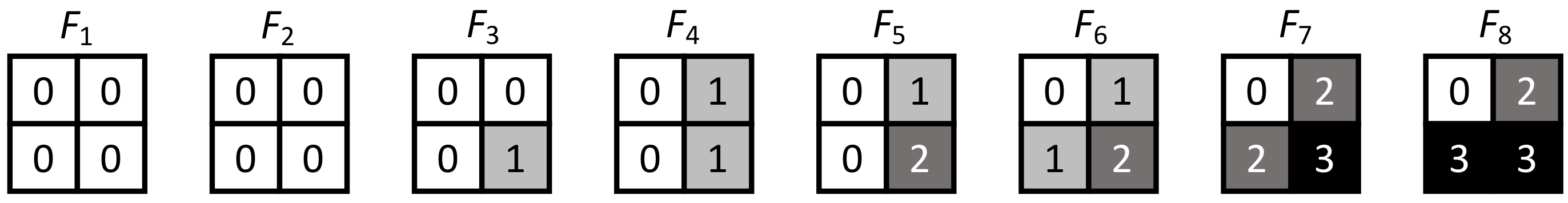
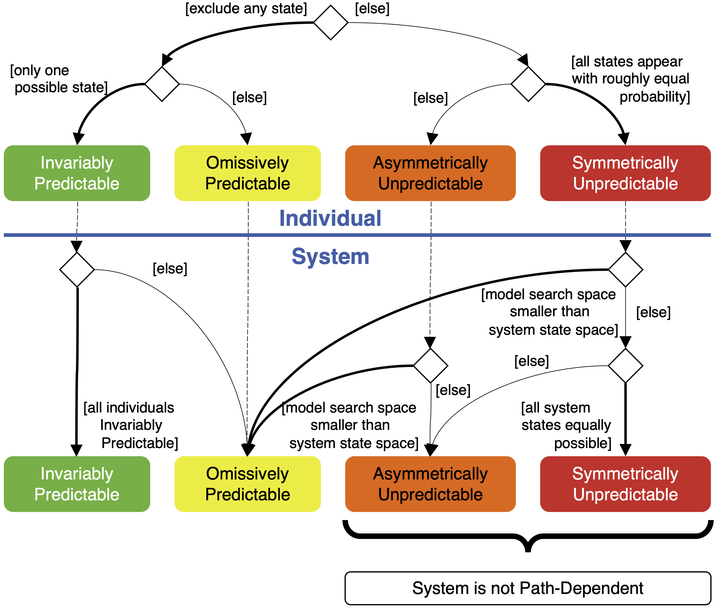
Figure 2 shows how the various predictability conditions in Table 1 are related to each other. It also highlights one argument for why prediction in complex systems should be possible: whole-system asymmetric and symmetric unpredictability should be ruled out by path dependence, which is stated explicitly by Thurner et al. (2018 p. 317) to be a possible inherent property of complex systems. In other words, if we find ourselves in a position where all possible states of a system are predicted by matching models to have non-zero probability, we might question whether that system is complex.
Rather more mundanely, system-level asymmetric and symmetric unpredictability require there to be at least as many matching (deterministic) models as there are states in the system. In the nondeterministic model case, the number of states in the system needs to be smaller than the product of the number of models and the number of alternative options generated by the stochasticity in each.
Thought experiment 1: Predicting cellular automata
Table 2 provides a summary of the prediction problem outlined in this thought experiment.
| Given | At least two consecutive snapshots of the CA’s space |
| The set of states each cell can have | |
| The neighbourhood of each cell | |
| Synchronous order in which cells compute their states | |
| Hidden | The transition function cells use to compute their states |
| Predict | The states of the CA \(M\) steps after the last snapshot |
| Outcome | Given enough data: invariable predictability, but exhaustive search is infeasible for all but the simplest CAs |
Imagine that someone has built a Class 4 (i.e. ‘complex’) CA that produces some interesting behaviour, but then forgotten the transition function. Luckily, they saved some images of that behaviour over \(N \ge 2\) time steps, they can remember the neighbourhood function returning \(C\) given cell \(i\), and they also recall the set of states \(K\). They are nevertheless curious about what the state of that CA would have been \(M\) steps later. As Langton (1990) points out, the space of transition functions is huge. Given there are \(\#K\) states that a cell can have, and \(\#C\) neighbouring cells, then the number of possible transition functions \(\#F\) is given by Equation 1.
| \[ \#F = \#K^{\left(\#K^{\#C}\right)}\] | \[(1)\] |
It is reasonable to assume that having recorded enough time steps (i.e. for \(N\) large enough), the absent-minded person would have sufficient information to narrow down the number of possible transition functions that faithfully reproduce the images generated by the CA to one. Ultimately, they would find the forgotten transition function of that CA, and by simulating it, they would generate the image the original would have produced \(M\) steps later. As the image was generated by simulation, we are not contradicting Wolfram by asserting that the image is our prediction for an image the forgotten transition function would have originally generated. Were the individual later to find the transition function they initially used, this prediction could even be verified.
Suppose \(N\) is not large enough to identify a single transition function that reproduces the \(N\)-long sequence of images, and instead there is a set of matching transition functions \(G\). We are interested in predictions for a finite subset of the image containing \(L\) cells at time \(T = N + M\). Table 3 then provides a specification for the four predictabilities in Table 1 at the individual cell and whole image levels.
| Un/Predictability | Cell | Image of \(L\) Cells |
|---|---|---|
| Invariable | All of the matching transition functions in \(G\) predict the same member of \(K\) for this cell at time \(T\). | All members of \(G\) predict the same image at time \(T\). |
| Omissive | At least one member of \(K\) never appears in this cell using any member of \(G\) at time \(T\). | At least one of the \(\#K^L\) possible images never occurs using any member of \(G\) at time \(T\). |
| Asymmetric | All members of \(K\) are possible in this cell at time \(T\), but with unequal proportions across all members of \(G\). | All of the \(\#K^L\) images are possible at time \(T\), but with unequal proportions across all members of \(G\). Note that the facts that each image is realized by at least one member of \(G \subseteq F\), and that at least one such state must occur more often than any of the others, means that \(\#F > \#K^L\), and hence, from Equation 1, \(\#K^{\#C} > L\). For \(L\) large enough, systemic asymmetric unpredictability is not possible. In elementary CAs, this happens when \(L > 2^3\). |
| Symmetric | All members of \(K\) occur in this cell at time \(T\) with equal proportions across all members of \(G\). | All of the \(\#K^L\) images occur at time \(T\) with equal proportions across all members of \(G\). To have a uniform distribution over the possible states at the systemic level, \(\#G = u\#K^L\), where \(u\) is a positive integer. |
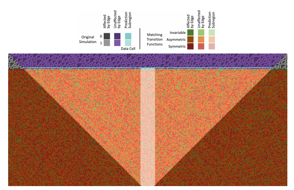
Though searching the space of transition functions might require more matter and time than the universe provides, the complexity of CAs, which has been argued for frequently, is not a theoretical obstacle to prediction. To demonstrate the principle and provide an explicit counter-example to the claim that complex systems are unpredictable, Figure 3 shows the output from a simulation that runs an elementary CA to get some data, and then tries to ‘find’ the transition rule used by exhaustively exploring all 256 transition rules, eliminating those rules that are not consistent with the data, and then plotting the predictability of cells using propositions 1 (green), 3 (orange) and 4 (red).7 (Individual cell omissive predictability is not an option when there are only two states.)
The cells shown in light blue in Figure 3 are ‘data’ cells, and there are two consecutive timesteps in which data are recorded. A minimum of two snapshots is needed to determine the transition rule using a method that relies on eliminating rules that do not reproduce later snapshots given earlier ones. The first snapshot has many more cells in it than the second. The width of the second snapshot is controlled by a parameter max-data, which in the run in Figure 3 is 21.
In the simulation depicted, the ‘real’ transition rule used to generate the data is rule 110 using ‘Wolfram code’ (Wolfram, 1983b); this rule is one of the most complex, proven capable of universal computation by Cook (2004). In the light-shaded region of the image (depicting the \(L\) cells) there are nevertheless cells coloured green throughout the run, illustrating that in this run at least, some cells are invariably predictable, even several time steps after the data.
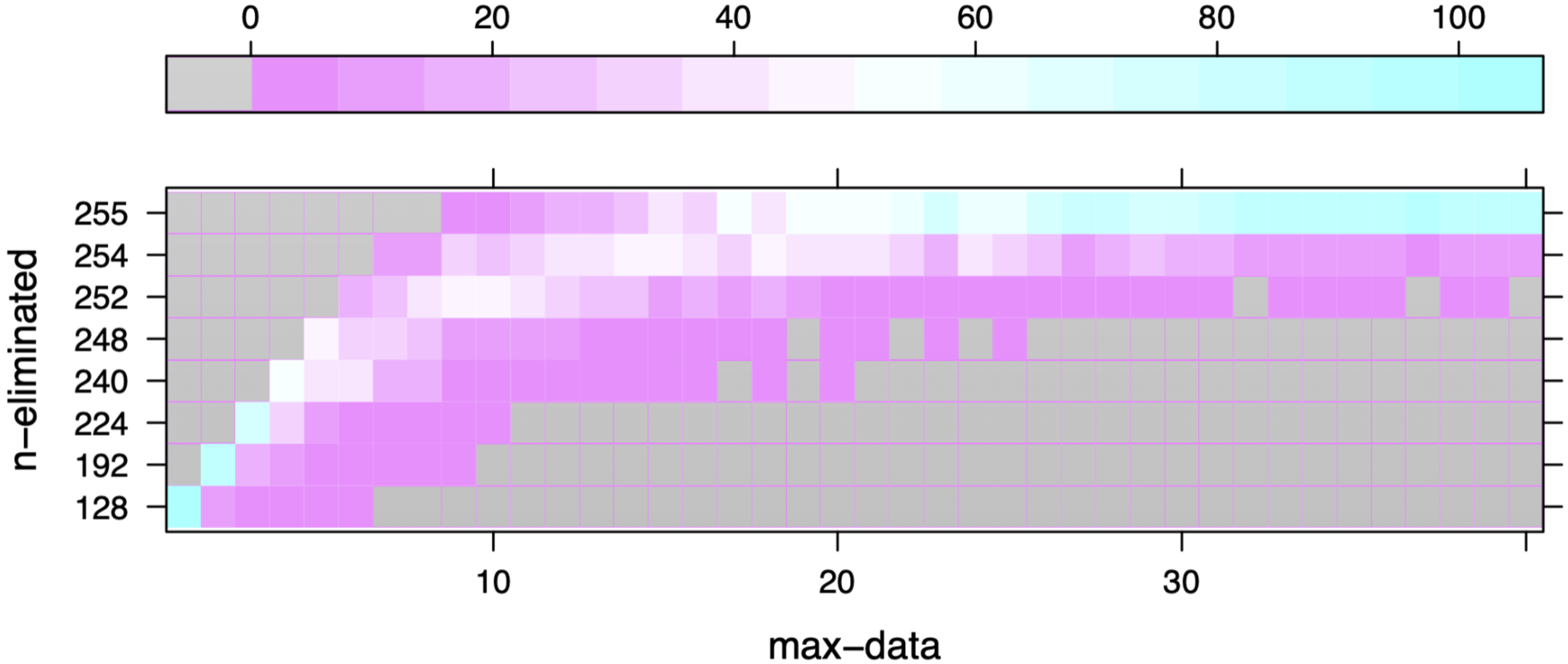
In Figure 4, the value of max-data is increased from 1 to 40, using 100 replications of each setting (4,000 runs in total), to show the relationship it has with the number of rules eliminated (n-eliminated). Of particular interest is the case where 255 rules are eliminated, as this shows when the ‘real’ rule (110) has been found, and all cells are invariably predictable. The results show that the majority of runs result in a singleton set \(G\) when max-data is around 20, with max-data needing to be more than 8 for this outcome to have occurred at all. Values of max-data between 30 and 40 rarely result in more than two members of \(G\), with a single member being found in a clear majority of cases.
Another point observable from Figure 3 is that the nature of the interdependencies of the cells means that, depending on the data provided and whether the CA is on an bounded grid, there is an inherent limit in how far ahead the prediction can be generated. For there to be no such limit, the CA must be bounded (in the case of the 1D CA depicted, the ‘tape’ of cells is joined at the ends so that it forms a ring), and at least one of the \(N\) snapshots must show the state of all cells in the tape. Otherwise, \(M\) is effectively limited as per Equation 2 by \(\#C\), \(L\) and the number of cells in the largest snapshot over the \(N\) timesteps, \(d^*\), with \(t^* \in [1, N]\) being the latest time step at which a snapshot of size \(d^*\) appears.
| \[ M \le \frac{d^* - L}{\#C - 1} - (N - t^*)\] | \[(2)\] |
Complication: Asynchrony
Table 4 summarizes the prediction challenge caused by what might appear to be a trivial complication to the CA. Note that in contrast with table 2, the transition function is now given, but we don’t know the order in which the cells compute their states.
| Given | \(N\) consecutive snapshots of the CA’s space |
| The set of states each cell can have | |
| The neighbourhood of each cell | |
| The transition function cells use to compute their states | |
| Hidden | (Non-computable) order in which cells compute their states |
| Predict | The states of the CA \(M\) steps after the last snapshot |
| Outcome | Simply computing the prediction itself rapidly becomes infeasible. |
In the CA thought experiment, each cell computes its state at time \(t\) based on the states of it and its neighbours at time \(t - 1\). Breaking that assumption builds asynchronous cellular automata, in which it is possible for the state of a cell at time \(t\) to depend on the state at time \(t\) computed by a neighbour that made the calculation prior to the cell in question. Critically, for our purposes, it must be impossible to write an algorithm that determines the order in which cells compute their state at time \(t\). Asynchronous CAs have been studied for many years (e.g. Ingerson & Buvel, 1984; Schönfisch & de Roos, 1999), with the argument that many of the ‘emergent’ effects of synchronous CAs are artefacts of synchrony. Even so, there are special classes of asynchronous CA that have been proven capable of universal computation in a similar manner to that of the rule 110 ECA (Yamashita et al. 2020).
It is not difficult to write an ABM that behaves in an analogous way. Suppose NetLogo used a true random number generator8 instead of the pseudo random number generator it uses in the ask command. Then, consider an instruction like the following:
ask turtles [
  forward [pcolor] of patch-here
  ask patch-here [
    set pcolor [color] of myself
  ]
]The scale of the computational problem posed by asynchrony for prediction should not be underestimated. For the purposes of illustration and comparison with the synchronous CA, imagine that we have somehow determined that rule 110 was the only rule that matched some data from an asynchronous variant of an elementary CA, and we now wish to predict the future state of the CA. Though there are various ways asynchrony can be implemented (Fatès 2013), a simple asynchronous variation of an elementary CA that is convenient for calculating the computational cost of prediction would have \(R\) cells arranged in a ring (such that cell 1 has cell \(R\) as its ‘left’ neighbour, and so cell \(R\) has cell 1 as its ‘right’ neighbour). Each step \(t\), the \(R\) cells would calculate their next state in a random order \(O_t\), such that \(O_{tj}\) is the cell computing its next state. Let the function \(\Omega_t(i)\) return the index \(j\) on \(O_t\) at which cell \(i \in \{1, 2, ... R\}\) computes its state. If \(\Omega_t(i) < \Omega_t(k)\) then cell \(i\) computes its state before cell \(k\) in step \(t\). The state of cell \(i\) at time \(t\) is then given by the state of cell \(i\) at time \(t - 1\), the state of cell \(i - 1\) at time \(t\) if \(\Omega_t(i - 1) < \Omega_t(i)\) and time \(t - 1\) otherwise, and the state of cell \(i + 1\) at time \(t\) if \(\Omega_t(i + 1) < \Omega_t(i)\) and time \(t - 1\) otherwise.
Since each ordering \(O_t\) is not computable, all \(R!\) possible orderings of the \(R\) cells should be explored. Worse, since the state at time \(t + 1\) depends on the specific state realized at time \(t\), to predict ahead \(M\) steps from the last snapshot at time \(N\), the number of orderings to explore is \((R!)^M\). This is exponential in both the number of cells9 and the number of steps ahead to predict. If \(R\) and \(M\) are both 10 (a small CA a short time ahead), the number of orderings to explore to accurately calculate the probability each cell has state 1 at time \(N + M\) is roughly \(4 \times 10^{65}\).
Thought experiment 2: Asynchronous networks of Turing Machines
Table 5 summarizes the prediction challenge in this thought experiment, which is based on several Turing Machines (TMs) operating asynchronously. This combines the challenges outlined in Tables 2 and 4 with more sophisticated computing power at the micro-level.
| Given | \(N\) consecutive snapshots of the TM’s tape |
| The alphabet of symbols each cell in the tape can have | |
| The number of agents \(p\) | |
| The size of the agents’ internal state set \(\#K\) | |
| Hidden | The transition function each agent uses to compute its next state, move, and write a symbol to the tape |
| The initial position on the tape of each agent | |
| The initial internal state of each agent | |
| (Non-computable) order in which agents compute their states | |
| Predict | The states of the tape \(M\) steps after the last snapshot |
| Outcome | Omissive predictability, but exhaustive search is infeasible, and handling the order being non-computable may mean asymmetric unpredictability is observed from the simulations even if this is not true of the underlying system. |
Agent-based models, insofar as they are defined, are computer simulations featuring a ‘sufficiently large’ number of agents each with their own attributes and simulated behaviour that can change their own attributes as well as those of other agents and, if included, a simulated, spatially-explicit environment (Polhill et al. 2019). The interactions of the agents form networks. Networks of autonomous agents acting in a shared physical environment can be considered to be like a set of TMs all operating on the same tape. Even though multiple TMs offer no more computing power than a single TM, writing a single TM that performs the same computation as the multiple TMs sharing a tape relies on knowing the order in which each of the multiple TMs act (or more precisely, that the order in which the TMs act is TM computable) (Copeland & Sylvan 1999). If this order is random (say, each of the multiple Turing Machines performs one step of computation each time a decay of a radioactive element is detected), the state of the tape at some point in the future is not computable in the general case.10
Despite not being able to compute the exact state of the tape at some point in the future, in this thought experiment, we imagine having \(N\) tape snapshots, and want to assess the predictability of the tape \(M\) steps later, where each ‘step’ is the execution of a single instruction by one of the TMs.
Turing Machines, like cells in cellular automata, have a finite set of internal states \(K\). However, the internal states are not ‘visible’ in this thought experiment. A TM also has a tape comprising an infinite number of discrete locations to which it reads and writes symbols from a finite alphabet \(A\), which must include a ‘null’ symbol (\(\emptyset\)). The null symbol in \(A\) is the default entry in a cell on the tape, which can only contain non-null symbol from \(A\) if the symbol is entered in the (finite) initial state of the tape, or if it is subsequently written by the TM. The tape is used to build the \(N\) snapshots in the thought experiment. Note that although a TM has an unbounded tape length, it is better to think of it as adding locations (with default state \(\emptyset\)) as needed. The portion of the tape from the left-most to the right-most non-null symbol is finite initially, and the machine can only move left or right one location in each step. Each of the \(N\) snapshots will be of finite length, therefore.
As noted in the introduction to this section, the transition function of a TM is a table of size \(\#K \times \#A\), each entry of which specifies: the symbol from \(A\) to write to the tape at the current location; the next state from \(K\) the TM should enter; and whether to move the read head left or right one position on the tape. Each entry could thus be any of \(2\#K\#A\) possibilities, and hence the number of possible state transition tables \(\#F\) is as shown in Equation 3.
| \[ \#F = (2\#K\#A)^{\#K\#A}\] | \[(3)\] |
In this thought experiment, we do not have information about the TMs in any of the \(N\) snapshots – neither about their state \(K\), nor about the position of their read-write heads on the tape. For the purposes of this thought experiment, we will allow ourselves the luxury of knowing the size of the TMs’ state set \(\#K\) used in the original snapshots.12 Some of the options we have to explore to exhaustively cover the ways in which the original snapshots might have been generated therefore pertain to the initial conditions. Let the left-most location on a tape \(x\) be whichever is the lesser of the left-most non-null symbol and the left-most location of a TM’s read-write head; and the right-most location \(y\) be whichever is the greater of the right-most non-null symbol or TM’s read-write head. The length of the tape is then \(1 + y - x\). If the length of the tape at the first of the \(N\) snapshots is \(l_1\), then for each of the possibilities in the transition function search space, the number of initial conditions to explore, \(s_I \le (l_1\#K)^p\); the inequality being a simplification for similar reasons to that for \(s_F\), albeit that in some combinations of state transition table, the order of assignment of initial condition to agent is important.
A further dimension of uncertainty arises from the fact that the order in which the \(p\) agents executed instructions when generating the \(N\) snapshots is not computable. However, in each of the \(N - 1\) steps, exactly one of the \(p\) agents executed an instruction, and so there are \(p^{N – 1}\) possible schedules to be explored. Let \(s\) be the number of options that need to be examined to find out what the state of the tape might be \(M\) steps after the last of the \(N\) snapshots. Then Equation 4 provides an upper bound for \(s\) that is, though intractably large to explore exhaustively, not infinite, and hence not undecidable.
| \[ s < (s_F s_I)^p p^{N – 1}\] | \[(4)\] |
| Un/Predictability | Cell | Tape |
|---|---|---|
| Invariable | For all members of \(Z\), for all \(g(z) \times p^M\) schedules, this tape location always has the same member of \(A\). | All of the \(L_T\) locations of the tape are invariably predictable. |
| Omissive | At least one member of \(A\) never appears at this tape location for all members of \(Z\) and \(g(z) \times p^M\) schedules. | At least one of the \(\#A^{L_T}\) possible tape configurations never occurs for all members of \(Z\) and \(g(z) \times p^M\) schedules. |
| Asymmetric | All members of \(A\) are possible in this tape location, but not with equal proportions across all members of \(Z\) and \(g(z) \times p^M\) schedules. | All of the \(\#A^{L_T}\) possible tape configurations are possible, but not with equal proportions across all members of \(Z\) and \(g(z) \times p^M\) schedules. |
| Symmetric | All members of \(A\) are equally possible in this tape location across all members of \(Z\) and \(g(z) \times p^M\) schedules. | All of the \(\#A^{L_T}\) possible tape configurations are equally possible across all members of \(Z\) and \(g(z) \times p^M\) schedules. |
The need to explore all possible initial conditions of the agents, together with conservative transition table elimination (only one of the possible schedules needs to match the \(N\) snapshots) make it more difficult for the data to be used to eliminate transition-table/initial-condition pairs. This makes it more likely that there will be variation in the predicted states of individual cells at time \(T\). Further, when making predictions, not knowing the schedule means all possibilities have to be explored. The definition of \(L_T\) allows for the possibility that the tape lengths of different predictions will not be the same. Hence, it is possible that the extreme left- and right-most positions of \(L_T\) will have \(\emptyset\) in some cases, and one or more other symbols from \(A\) in others. If so, at least these positions will not be invariably predictable, and systemic invariable predictability will not apply. For similar reasons, systemic symmetric predictability also seems unlikely, as from Figure 2, systemic symmetric unpredictability is a subset of the cases where all individuals are symmetrically unpredictable. For an extreme location on the table to be individually symmetrically unpredictable, any option not using one of the extreme locations on the tape needs to be matched with exactly \(\#A - 1\) options using each of the other symbols in \(A\) in that location, with the remaining options all using elements of \(A\) in equal proportions.
If we maintain the argument that path-dependence means systemic asymmetric and symmetric unpredictabilities are inconsistent with the system under study being a complex system, and regard systemic invariable predictability as a negligible possibility for the reasons given above, omissive predictability is the only outcome at whole system level. The situation is more complicated, however, because we explore all the \(p^M\) schedules when making the prediction, when some might be impossible in the real world: non-computability of the schedules doesn’t necessarily mean all schedules are possible, only that we can’t build a TM to calculate what the actual schedule is, and hence need to check the outcomes from all the possibilities.13 The predicted results might therefore be asymmetrically unpredictable even if the original system is complex and path-dependent.
Complication: Wicked systems
| Given | \(N\) consecutive snapshots of the TM’s tape |
| A partial alphabet of symbols each cell in the tape can have | |
| The number of agents \(p\) | |
| Hidden | The transition function each agent uses to compute its next state, move, and write a symbol to the tape |
| The initial position on the tape of each agent | |
| The initial internal state of each agent | |
| Order in which agents compute their states | |
| The full size of the agents’ internal state set | |
| Additional symbols in the alphabet for the future systems | |
| Predict | The states of the tape long enough after the last snapshot that none of the symbols in the partial alphabet appear |
| Outcome | Symmetric unpredictability with an infeasibly large search space |
The difficulties with predicting states of a system are not only due to complexity. The related literature on social-ecological systems describes some systems as ‘wicked’ (Andersson & Törnberg 2018), based on Rittel and Webber’s (1973) definition of ‘wicked problems’. The concept of ‘wicked problems’ is used by Rittel & Webber (1973) to explain why conventional, i.e. rational analytical, approaches fail to understand social-ecological systems in reality, for example, in urban planning. Following Zellner & Campbell (2015) and abstaining from the parts that are more specific to public policy and planning14, the criteria can be summed as follows: First, there is no definitive formulation of a wicked problem. Second, there is no definite solution to a wicked problem, since the solution may generate cascading waves of repercussions, e.g. positive feedback effects, and/or is a symptom of another problem. Third, there is no clear set of potential solutions nor a well-described set of permissible operations. Fourth, related to the first criterion, the wicked problem can be explained in numerous ways. Fifth, every wicked problem is unique.
From these criteria, it follows that complexity is considered to be an integral part of wicked problems in the applied literature (e.g., Batie 2008, Zellner & Campbell 2015 and Head 2008) as well as in systems research (Andersson et al. 2014; Andersson & Törnberg 2018). For Head (2008), for example, wicked problems in real social-ecological systems, e.g. political systems, are determined by complexity (subsystems and their interdependencies), uncertainty (unknown consequences of action and changing patterns) and divergence (fragmentation in viewpoints). Complexity is thus a necessary, but not sufficient, criterion for wickedness.
From a systems perspective, Andersson et al. (2014) and Andersson & Törnberg (2018) characterize wicked systems as ones in which wicked problems arise. Wicked systems combine two system distinct qualities, complicatedness and complexity. A complicated system is viewed to have a large number of components that behave in a well-understood way and have well-defined, but distinctive roles leading to the resulting effect. Typical examples are usually machines such as helicopters or aeroplanes, which have millions of physical parts (San Miguel et al. 2012). The components of complicated systems are decomposable in that they can be analysed individually. Complex systems may also have a large number of components, but each component is of the same kind (as in the cells of a CA), or at least, the number of classes of component is considerably smaller than in wicked systems. However, the interactions among the components lead to collective or systemic emergent behaviours that cannot, even qualitatively, be derived from knowledge of the individual components’ behaviour (San Miguel et al. 2012). The components of a complex system are thus not decomposable in the way they are in a complicated system, since the complex system would lose its emergent features and the single components their relatedness. Wicked systems combine both qualities, complexity and complicatedness. The interactions among the components hamper analyses of the the rules of a single component.
The analysis in the second (TM) thought experiment assumed knowledge of a system that might not generally be the case in real-world problems: the number of agents \(p\), the alphabet of the tape \(A\), and set of states agents might have \(K\) could all be unknown. The \(N\) snapshots might not cover the whole tape. Andersson & Törnberg (2018 p. 124) emphasize the uncertainty of wicked systems, noting that this includes “ontological uncertainty”. There are various ways “ontological uncertainty” could be occur, which we expand on below. First, there could be what might be called ‘representative ontological uncertainty’, in which there is no single way to represent the system that is obviously ‘right’ or agreed on by everyone. Second, ‘empirical ontological uncertainty’ applies where there is disputation over the data to be used to model the system. Third, and more significantly, ‘endogenous ontological uncertainty’ raises the possibility that novel system states emerge as the system evolves.
In the context of the TM thought experiment, representative ontological uncertainty pertains to such things as what the alphabet of the tape might be (beyond those symbols already observable from the snapshots), or what states agents could have (though really, it is only the maximum number of states they could have that matters). If there are a finite number of alternative representations, then the problem of exploring the space of transition tables that match the data is the product of the problems of exploring each single representation. It is then that much more intractable, but still not undecidable.
Empirical ontological uncertainty would be interpreted as disputation about the validity and appropriateness of the \(N\) snapshots as being the only data by which possible models of the system are rejected. While debate about the alphabet of symbols \(A\) is more a question of representative ontological uncertainty, arguments about which element of \(A\) should be used in each initial location would be a question of empirical ontological uncertainty. In general (beyond the immediate context of the TM thought experiment), empirical ontological uncertainty arises from disputation among domain experts in the wicked system, whose knowledge might be sought when attempting to model it. One way to address such uncertainty is to run the multiple alternative models with any of the multiple different initial conditions with which they are compatible. Even so, if the number of alternatives to explore is finite, prediction based on exhaustive search of alternatives is ruled out on the grounds of tractability not decidability.
However, if it was unlikely before that invariable system-level predictability would occur, it becomes vanishingly small as the number of alternative representations and initializations to explore increases. On the other hand, the fact that the different representations will not lead to all symbols on the tape occurring in every matching run means that cell-level symmetric unpredictability becomes increasingly unlikely too, and with it, systemic asymmetric or symmetric unpredictability. At the whole-system level, omissive predictability is then by far the most likely, if not the only, option.
One feature of wicked systems clear from Andersson & Törnberg (2018) is endogenous ontological uncertainty: the dynamics of the system itself lead to the creation of novel states, agents, and symbols. Computationally speaking, this is not the obstacle it might at first appear to be, as the new agents can initially run TM transition rules that effectively make them inactive until they are needed, and the novel states and symbols can be provided in extended sets, with special transition rules activated under whatever conditions it is that leads to the updated ontology applying. These add exponentially to the intractability of modelling the system, but do not make the task undecidable. However, this misses the point. The real issue with wicked systems pertains to the data available when the prediction is needed.
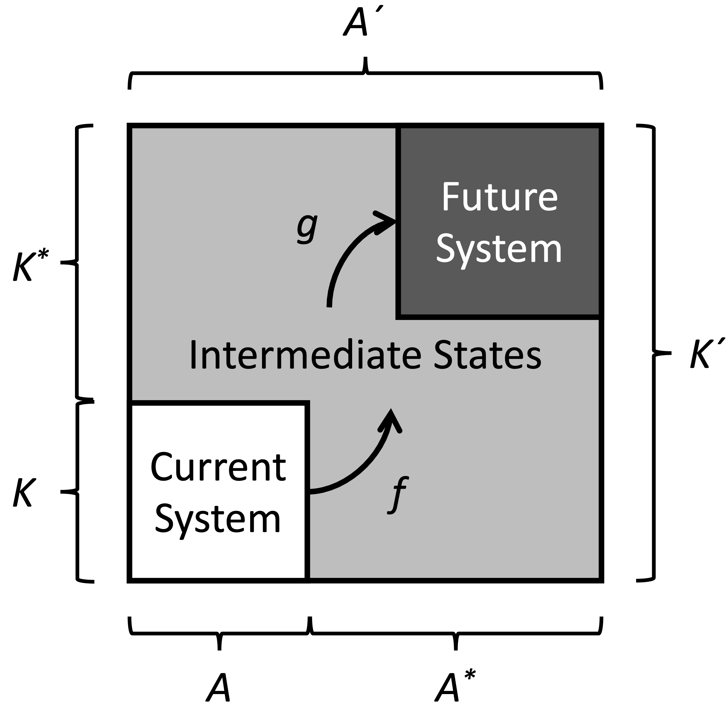
To extend the thinking in the second thought experiment, we now imagine a finite alphabet \(A^\prime = A \cup A^*\) and finite set of states \(K^\prime = K \cup K^*\), where no member of \(A^*\) appears in any of the \(N\) snapshots, and no member of \(K^*\) appears as any of the initial states of the TMs. \(A^*\) and \(K^*\) thus represent the endogenous ontological uncertainty, but we have no data about them in the \(N\) snapshots used to determine which models will generate our predictions. Hence, even though we might narrow down the set of transition functions and orderings of TM activities that reproduce the \(N\) snapshots on the tape, all options for transition functions involving states in \(K^*\) and reading or writing symbols on the tape in \(A^*\) are open (see Figure 5). Assuming the emergent new system is expected only to involve states and symbols that are proper subsets of \(K^*\) and \(A^*\), then even though strictly speaking with respect to \(A^\prime\) the whole system is omissively predictable, with respect to the subset of \(A^*\) that would usefully give us information about the expected new state of the system, the tape is symmetrically unpredictable. Effectively, endogenous novelty creates the conditions in which, even if we could exhaustively explore the space of all possible models we could build to see how they fit the data we have in the present, the exercise is futile in that Edmonds’s (2017; 2019a) definition means there is no useful degree of accuracy by which predictions can be made once the symbols in \(A\) and states in \(K\) are no longer relevant. The emphasis is important because there is still potential utility in modelling wicked systems in providing the scope for detecting or estimating when the current system (\(A\), \(K\) and associated transition functions) is shifting away from its current basin of attraction.
One case where the capability to simulate the emergence of novelty would be useful is in the exploration of scenarios involving ‘Transformative Social Innovations’ (Avelino et al. 2019). Social Innovations are “new ways of doing, organizing, framing and knowing” (Avelino et al. 2019 p. 197), while Transformative Social Innovations are “Social Innovation that challenges, alters or replaces dominant institutions in a social context” (Avelino et al. 2019 p. 196), and is an inherently coevolutionary concept. However, other less extreme examples include scenarios exploring the introduction of new technology to a system, or new policies, and the ways in which agents might adapt and respond to them. Filatova et al. (2016) argue that regime shifts can occur gradually, grown within a system, as well as shocks or perturbations to an existing system. If the only data we have (including description of the system itself) when modelling pertains to the current system, we are obviously in a difficult position if we want to predict what a new system might look like.
Clearly, then, agent-based models of wicked systems need to have agents with the potential to create novelty, or (minimally) to allow for the possibility that there is an ‘escape’ from the transition rules that dynamically generate states within the space of the current system. Mitchell’s (2009 p. 13) characterization of complex systems as having “simple rules of operation” for its agents, cited in the introduction, is insufficient for wicked systems insofar as such simplicity does not entail the potential to create new rules and states. Andersson et al. (2014), however, acknowledge that Edmonds and Moss’s (2005) ‘descriptive’ agent-based modelling style (in contrast to the SFI-school’s ‘KISS’ – Keep It Simple, Stupid) increases the complicatedness of the systems to which agent-based modelling can be applied towards tackling wicked rather than purely complex systems.
Discussion
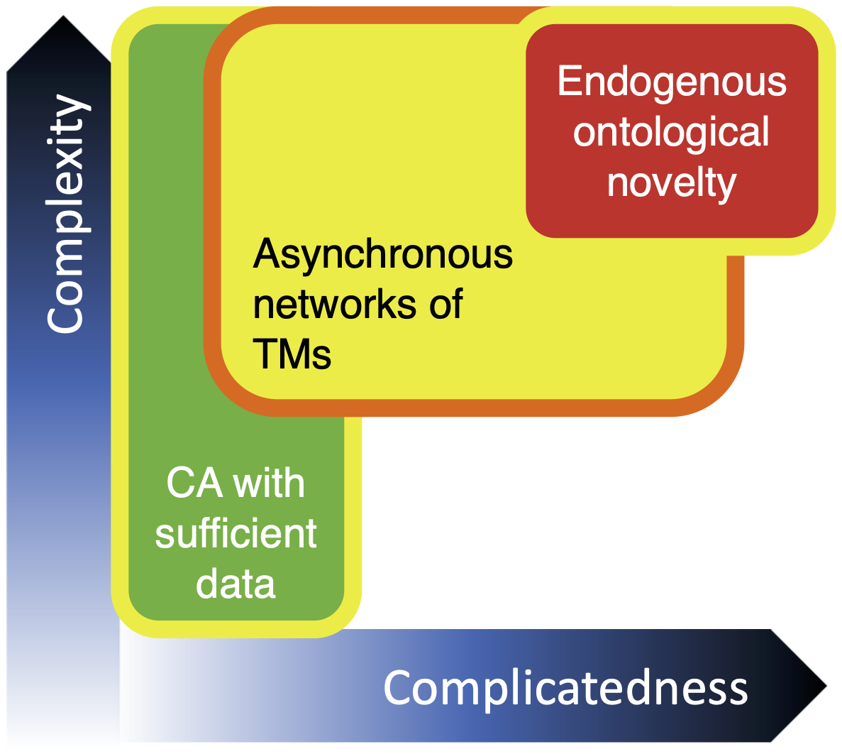
In this article, we have defined four levels of predictability, and related them to usefulness with respect to possible system states predicted to occur or not to occur. After some general considerations, we have then evaluated these predictabilities in complex and wicked systems. Figure 6 summarizes those findings. We have also shown that the search spaces of models of complex systems are finite and that in the very simplest case of an elementary CA with rule 110, which is classified as ‘complex’ and proven capable of universal computation, the search space is small enough that we can find the original rule from snapshot data by exhaustive search.
The network of asynchronous TMs thought experiment in Section 2.3 is a worst-case that maximizes the computational power of the interacting agents, and includes an element of non-computability with respect to the ordering of their execution on the shared tape. As Copeland & Sylvan (1999) observe, just two TMs writing asynchronously to the same tape could be in the process of computing a non-computable number. Such asynchrony is not infeasible empirically, as in the real world agents act autonomously. This point challenges the idea that even a model that perfectly reproduces historical data can automatically be trusted to make point predictions in systems with analogous properties. Numerical validation cannot, on its own, be trusted as the basis for accepting a model’s prediction in such systems – we need other criteria, such as assessments of ontological structure (Polhill & Salt 2017). The implication of this for trusting predictions is that validity pertains to the representation of the system as well as numerical accuracy.
As made apparent by the application of the asynchronous TMs thought experiment to wicked systems in Section 2, it is endogenous ontological uncertainty that poses the most significant challenge to prediction. The problem, however, is not one of computability, but of data. Indeed, even in the first thought experiment with deterministic cellular automata, if the \(N\) images do not include all of the states \(K\), the uncertainty about cells’ states will increase as fewer possible transition functions are ruled out. In much the same way as the complete works of Shakespeare make no reference to smartphones, endogenous novelty means that presently available data provide less and less information about the future the further ahead predictions are required. Generalizing this thinking from cellular automata shows that, when present states give you no information about relevant future states (i.e. \(K^\prime = K \cup K^*\); \(K \cap K^* = \emptyset\) and the states of \(N\) only contain elements of \(K\)), systems can be unpredictable even if they are deterministic.
This line of thinking sheds new light on McDowall and Geels’s (2017) commentary on an article by Holtz et al. (2015) outlining the cases for using agent-based models to simulate societal transitions. McDowall & Geels (2017) draw on the conceptualization of wicked systems by Andersson et al. (2014) to argue that Holtz et al. (2015) underestimate the depth of the challenge of simulating societal transitions, and reference Bai et al. (2016) in support of the statement that systems change their structure. Holtz et al. (2015) make no claim that the contribution agent-based modelling can make to the transitions discourse is predictive; rather they articulate the benefits around explicit specifications, capturing emergent dynamics, and systematic exploration of scenarios (pp. 43-44). However, they also give a use case of giving advice to policymakers (ibid., pp. 46-47), which leads McDowall & Geels (2017 pp. 42–43) to raise challenges in relation to how models are interpreted, used and trusted in decision-making processes. Our analysis suggests that trust based on fitting conditions in the current system cannot be generalized to trusting what the models say about the transitioned system. We have also added weight to thoughts McDowall & Geels (2017 p. 45) express based on Byrne & Callaghan (2014)’s observations about styles of agent-based modelling that are akin to the SFI-school of complexity – emergence of structures from agents with simple decision rules – that wicked systems are more complicated than these models are suited to. Agent-based models of wicked systems need somehow to address novelty.
The philosophy surrounding the role, building, verification, validation and use of simulation modelling in general (rather than specific to ABM) has been debated for over half a century. The epistemological divides are often silo-related. An engineer using ABM has very few philosophical qualms about using it for prediction, but this paper addresses novelty in ABMs in the context of wicked problems – where many social scientists rather than engineers are building ABMs. The epistemological tension of building models for prediction within science is summarized well by Babuska & Oden (2004), and we direct the reader there for an overview of this debate. The importance of this debate for this paper, however, is that absolute (in the sense of being objective, or universally agreed) verification and validation of ABMs need not be achieved for prediction to be useful, even in the case of introducing novelty in systems.
In his Nobel Prize lecture reflecting on The Pretence of Knowledge in complex societal systems, Hayek (1974) said, “The real difficulty, to the solution of which science has little to contribute, and which is sometimes indeed insoluble, consists in the ascertainment of the particular facts.” It is worth considering the degree to which it is realistic that the information assumed in the search problems outlined in section 2.1 and, since it is intended as a metaphor for coupled multi-agent social and environmental systems, especially section 2.3 would ever be available in empirical situations. Use of cellular automata to model social systems has a long history, particularly in land use and urban systems (Batty et al. 1999; Clarke & Gaydos 1998; White & Engelen 1993) (albeit with some deviation from the strict definition of cellular automata (O’Sullivan & Torrens 2001)), and a recent review of calibration and validation methods (Tong & Feng 2020) suggests it continues to be a popularly-used method. Spatial data from mapping, aerial photography and satellites offer rich, time-varying data that can be used for empirical applications of such models. It does not seem implausible that the \(N\) snapshots of data would be available in the case study, then, but not necessarily in consecutive timesteps. The CA thought experiment also assumed, however, that the set of states \(K\) and the neighbourhood of each cell \(C\) was known. While the states could perhaps be inferred from the classifications of polygons and/or pixels in GIS data,15 ‘neighbourhood’ is more than a spatial concept for the purposes of land use change, since the scope of influence on the state of a cell is not purely that of other cells with which it happens to share a boundary.
In the asynchronous networks of TMs example, we allowed the state of the whole tape to be available after each time an agent acted, along with the alphabet of symbols on the tape \(A\), the population of agents \(p\), and the number of internal states of the TMs \(\#K\). The initial positions of the agents, and their specific internal states were not provided. If we see the tape as representing the state of the biophysical environment (including an embodiment of aspects of the agents’ memories), then besides the point raised with respect to CAs that snapshots will not be available after each of a number of consecutive actions, we should also not expect all the data at any one time to be available. Knowing the number of internal states of the TMs is also unrealistic. Though the advent of ‘Big Data’ (Gandomi & Haider 2015) might mean lack of data would be regarded with skepticism, issues with it such as ‘Veracity’ (questionable provenance, accuracy and quality), ‘Volatility’ (limited life-span) and ‘Variety’ (heterogeneous and unstructured) among other ’V’s (Khan et al. 2018) do not make it necessarily suitable for work with ABMs.
Hayek (1967) response to the lack of data in complex societal systems was to argue for “pattern prediction”:16 recurring well-defined classes of event, and such things as the classes of event that presage their occurrence or the conditions needed to make them happen. These, as Hayek notes, are falsifiable theories, and in ecology, Grimm et al. (2005) have advocated the replication of patterns as a validation criterion in the specific context of agent-based models. The thought experiments were deliberately constructed in abstract rather than empirical systems so that their inherent complexity could be evaluated as a difficulty with prediction, and data availability and questions about representing the target system not be an obstacle or confounding factor.
The justification for more complicated agent-based models in empirical contexts has already been argued by Sun et al. (2016). However, the quality of the complications needed for wicked systems with respect to various aspects of the model’s ontology highlighted here relates to addressing the issue of novelty. There are several ways in which agent-based models can and do provide for novelty. Polhill et al. (2016 p. 319) outline three levels of systemic change. At the simplest level, \(\Delta E\), is a change in the entities simulated, which can occur through simulation of processes such as the birth and death of agents, and the creation and destruction of links. A more substantive change, \(\Delta P\), involves changes to the processes. One approach already used in some models is embedding machine learning algorithms in agents’ decision-making algorithms. These algorithms adjust the mechanisms by which agents make decisions based on their experiences operating in the model. Though they change the way in which agents decide what to do, they don’t provide for innovation of completely new actions, which is possible given a model in which actions could be aggregations of more elementary movements around which agents could reason goal-oriented plans. The most challenging level of change, \(\Delta L\), entails endogenous adjustments to the language used to describe the model itself: the spontaneous creation of new classes of entity, new attributes, new relationships, and new institutions for collectives of agent. We are not aware of any models that provide such functionality, but note work such as that of Gessler (2010) in the Artificial Life community outlining such an agenda.
Our observations about prediction in wicked systems are predicated on current data about the system becoming obsoleted by novel states in the future about which there is no information in the system as it is now. Knowledge elicitation methods that anticipate what those states might be could be one way to obtain these kinds of data. García-Mira et al. (2017), for example, use backcasting (Quist & Vergragt 2006) to elicit scenarios for agent-based models to explore. Narrative approaches can also be used as sources of qualitative data for models. However, this constitutes an epistemological shift in the underpinning of the model – is it a scientific artefact and/or a tool to facilitate dialogue? McDowall & Geels (2017) caution modellers to be clear about the difference and mindful of the philosophies of science at play, whilst Gilbert et al. (2018 para. 5.26) observe that there can be pressure from policymakers to understate uncertainties such as those arising from these considerations. Using knowledge from stakeholders to determine potential future system states that form the basis of agent-based model designs arguably entails a constructivist philosophical perspective (McDowall & Geels 2017 p. 46). Hassan et al. (2013), who also draw attention to the 2008-09 debate about prediction referenced in the introduction, introduce the social simulation community to the forecasting literature. Hassan et al., who make no distinction between forecasting and prediction (2013 para. 2.1), draw on Armstrong (2001), translating his 139 principles of forecasting into twenty guidelines suitable for evaluating in an agent-based modelling context. Critically, many of these guidelines entail documenting the social processes of building, using and evaluating the model. Documenting the social processes of model construction and use of data when making predictions records how a particular community addressed the wickedness of the system they were interested in, and makes explicit the intersubjectivity (Cooper-White 2014) of any predictions. Ahrweiler (2017 p. 411), in an article concluding that ABMs offer what she calls ‘weak prediction’, observes that, “To trust the quality of the simulations means to trust the process that produced its results. This process is not only the one incorporated in the simulation model itself. It is the whole interaction between stakeholders, study team, model, and findings.”
Conclusion
Path dependency in complex systems mean they are predictable at the whole-system level in theory, if not in practice because of the intractability of exhaustively searching the space of models that might match the available data. Wicked systems, however, pose a much more significant challenge to prediction, chiefly as a consequence of endogenous ontological novelty, rather than disputation about ontological structure. Beyond the short term, the (potential) introduction of novel states in the system about which there are no data at the time the prediction is made means attempts at prediction are futile even if they were feasible. Though there are other purposes than prediction for building a model, there is still predictive utility to be had in modelling the current system and using this to detect transitions as the real world diverges from the states represented in the model. The social processes of constructing models in wicked systems mean that ‘intersubjective prediction’ is a more meaningful term. Models of wicked systems, however, need to be more complicated than complex systems, and should include functionality that allows for novelty.
Acknowledgements
This paper is derived from a paper presented to SSC 2019 in Mainz, Germany. Work in this paper has been supported by The Scottish Government Environment, Agriculture and Food Strategic Research Portfolio 2016-2021 (Theme 2: Productive and Sustainable Land Management and Rural Economies); The Macaulay Development Trust (Project no. E000956); the European Commission’s Horizon 2020 project SMARTEES (grant agreement no. 763912); and the Research Council of Norway (project nos. 244608 and 294777). We are grateful to three anonymous reviewers for their constructive and challenging comments on earlier drafts of this article.Notes
- At the time of writing, no response to that challenge has been received.↩︎
- Stronger criteria for usefulness could be defined with respect to sets of states, given matching criteria that allowed each set to be defined. A prediction would then only be possibly useful if it confirmed all members of a set of states were possible, or all members of a set were not possible. This would go some way to capturing the “accuracy” aspect of the definition provided by Edmonds et al.(2019a). The weaker definition used here makes the assertion of uselessness of a prediction (such as in section 2.4 on wickedness) stronger, however.↩︎
- There is still a certain difficulty with this understanding of prediction. Imagine a model is used in 2020 to make a large enough number of “statements” about the situation in the year 2100 that \(W\) (the proportion of such statements that prove not to be usefully accurate) can be estimated. The status of those “statements” when made in 2020 as predictions cannot be verified until 80 years into the future. In the commonsense world, predictions can be wrong all the time, but still be predictions. (Wikipedia maintains a list of predictions of the end of the world, for example.) That would not be helpful in this article, as the scope of predictive models would include random number generators, astrology, and reading tea-leaves.↩︎
- The fact that models used in this context are then parts of the system that they are predicting could then used as an argument against the possibility of prediction, as there is an apparent infinite regress of a model needing to embed responses to its own predictions in its predictions. However, adaptive control mechanisms (see Nise (2004)) are already an example of models embedding themselves in the systems they are simulating, suggesting this isn’t necessarily the obstacle to prediction it might appear. The matter is also touched on by Nagel (1979 p. 468), who notes that predictions can be ‘suicidal’ when action taken to respond to them means they do not occur. This doesn’t change their status as a prediction. To make the matter explicit, consider the predicted effects of climate change if human societies take insufficient action to curb greenhouse gas emissions, which are intended to provoke action to avoid them coming true (Hoegh-Guldberg et al. 2018). We would not argue that these weren’t predictions, nor would we support any definition of prediction for which they did not qualify.↩︎
- Even if chaos theory does not apply to an ABM, the need for infinite precision is highlighted by various authors discussing floating-point arithmetic (Hegselmann & Krause 2015; Izquierdo & Polhill 2006).↩︎
- Building a TM to simulate an ABM, or even a single agent, would be somewhat tedious. The point is that a TM is computationally equivalent to an agent, and has a structure for the transition table that is convenient for calculating model search space size.↩︎
- Code for this NetLogo model is available in a GitHub repository at https://github.com/garypolhill/prediction-CA.↩︎
- Hardware for true random number generation is available, and websites such as https://www.random.org/ are available providing access to true random numbers.↩︎
- See Stirling’s approximation to \(n!\)↩︎
- Networks of asynchronous Turing Machines could be simulated using a so-called ‘Oracle Machine’ – essentially a Turing Machine with a ‘black box’ fitted that can magically provide the correct Boolean answer to a question posed of it. Here, the Oracle Machine would be used to indicate whether it was a particular agent’s turn to run an instruction. Computer scientists have applied Oracle Machines to the question of whether \(P \overset{?}{=} NP\) (e.g. Gaßner 2008). Here, however, we are interested in the implications of a set-up such as this for predictability without the advantage of an Oracle.↩︎
- Assuming all agents can follow different instructions, and the order of assignment of state transition table to agent does not matter.↩︎
- This is quite a luxury. Without it, we’d have to start with \(\#K = 1\) (or \(2\) if \(K\) includes
HALT) and increase \(\#K\) until we were able to replicate the \(N\) snapshots. Even having found a replicating case, we would not be confident that the value of \(\#K\) found was the value of \(\#K\) from the original system, and could only rely on heuristics such as Ockham’s Razor to justify not exploring higher values of \(\#K\). However, not knowing \(\#K\) could be argued to be a data issue rather than a problem derived specifically from the complexity of the system we are trying to recover.↩︎ - An example of such a situation would be where agent \(1\) always executes an instruction after agent \(2\), with agents \(2 ... p\) triggered on radioactive decay.↩︎
- For example, criterion no. 10: The planner has no ‘right to be wrong’, i.e. there is no public tolerance of initiatives or experiments that fail.↩︎
- Given observations by authors such as Chazdon et al. (2016) about definitions of what might seem fairly trivial land use concepts (in this case ‘forest’), the task of identifying cell state symbol sets to use in a CA of land use change should not be underestimated.↩︎
- We are grateful to Reviewer #2 for pointing us in the direction of this work.↩︎
References
AHRWEILER, P. (2017). Agent-based simulation for science, technology, and innovation policy. Scientometrics, 110, 391–415. [doi:10.1007/s11192-016-2105-0]
ANDERSSON, C., Törnberg, A., & Törnberg, P. (2014). Societal systems – complex or worse? Futures, 63, 145–157. [doi:10.1016/j.futures.2014.07.003]
ANDERSSON, C., & Törnberg, P. (2018). Wickedness and the anatomy of complexity. Futures, 95, 118–138. [doi:10.1016/j.futures.2017.11.001]
ANZOLA, D. (2019). Disagreement in discipline-building processes. Synthese. [doi:10.1007/s11229-019-02438-9]
APPEL, K., & Haken, W. (1977). Every planar map is four colorable. Part I: Discharging. Illinois Journal of Mathematics, 21(3), 429–490. [doi:10.1215/ijm/1256049011]
APPEL, K., Haken, W., & Koch, J. (1977). Every planar map is four colorable. Part II: Reducibility. Illinois Journal of Mathematics, 21(3), 491–567. [doi:10.1215/ijm/1256049012]
ARMSTRONG, J. S. (2001). Principles of Forecasting: A Handbook for Researchers and Practitioners. Norwell, MA: Kluwer Academic Publishers.
AVELINO, F., Wittmayer, J. M., Pel, B., Weaver, P., Dumitru, A., Haxeltine, A., Kemp, R., Jørgensen, M. S., Bauler, T., Ruijsink, S., & O’Riordan, T. (2019). Transformative social innovation and (dis)empowerment. Technological Forecasting and Social Change, 145, 195–206. [doi:10.1016/j.techfore.2017.05.002]
BABUSKA, I., & Oden, J. T. (2004). Verification and validation in computational engineering and science: Basic concepts. Computer Methods in Applied Mechanics and Engineering, 192(36–38), 4057–4066. [doi:10.1016/j.cma.2004.03.002]
BAI, X., van der Leeuw, S., O’Brien, K., Berkhout, F., Biermann, F., Brondizio, E. S., Cudennec, C., Dearing, J., Duraiappah, A., Glaser, A., M.and Revkin, Steffen, W., & Syvitski, J. (2016). Plausible and desirable futures in the Anthropocene: A new research agenda. Global Environmental Change, 39, 351–362. [doi:10.1016/j.gloenvcha.2015.09.017]
BATIE, S. S. (2008). Wicked problems and applied economics. American Journal of Agricultural Economics, 90(5), 1176–1191. [doi:10.1111/j.1467-8276.2008.01202.x]
BATTY, M. (2020). Unpredictability. Environment and Planning B: Urban Analytics and City Science, 47(5), 739–744. [doi:10.1177/2399808320934308]
BATTY, M., Xie, Y., & Sun, Z. (1999). Modeling urban dynamics through GIS-based cellular automata. Computers, Environment and Urban Systems, 23, 205–233. [doi:10.1016/s0198-9715(99)00015-0]
BYRNE, D. (1998). Complexity Theory and the Social Sciences. London: Routledge.
BYRNE, D., & Callaghan, G. (2014). Complexity Theory and the Social Sciences: The state of the Art. London: Routledge.
CHAZDON, R. L., Brancalion, P. H. S., Laestadius, L., Bennett-Curry, A., Buckingham, K., Kumar, C., Moll-Rocek, J., Guimarães Vieira, I., & Wilson, S. J. (2016). When is a forest a forest? Forest concepts and definitions in the era of forest and landscape restoration. Ambio, 45, 538–550. [doi:10.1007/s13280-016-0772-y]
CLARKE, K. C., & Gaydos, L. J. (1998). Loose-coupling a cellular automaton model and GIS: Long-term urban growth prediction for San Francisco and Washington/Baltimore. International Journal of Geographical Information Science, 12(7), 699–714. [doi:10.1080/136588198241617]
COOK, M. (2004). Universality in elementary cellular automata. Complex Systems, 15(1), 1–40.
COOPER-WHITE, P. (2014). 'Intersubjectivity.' In D. A. Leeming (Ed.), Encyclopedia of Psychology and Religion (pp. 882–886). Boston, MA: Springer US. [doi:10.1007/978-1-4614-6086-2_9182]
COPELAND, B. J., & Sylvan, R. (1999). Beyond the universal Turing machine. Australasian Journal of Philosophy, 77(1), 46–66. [doi:10.1080/00048409912348801]
DAVIES, K. K., Fisher, K. T., Dickson, M. E., Thrush, S. F., & Le Heron, R. (2015). Improving ecosystem service frameworks to address wicked problems. Ecology and Society, 20(2), 37. [doi:10.5751/es-07581-200237]
DE MATOS Fernandes, C. A., & Keijzer, M. A. (2020). No one can predict the future: More than a semantic dispute. Review of Artificial Societies and Social Simulation. Available at: https://rofasss.org/2020/04/15/no-one-can-predict-the-future/.
EDMONDS, B. (2017). 'Different modelling purposes.' In B. Edmonds & R. Meyer (Eds.), Simulating Social Complexity: A Handbook (pp. 39–58). Berlin Heidelberg: Springer International Publishing. [doi:10.1007/978-3-319-66948-9_4]
EDMONDS, B., Le Page, C., Bithell, M., Chattoe-Brown, E., Grimm, V., Meyer, R., Montañola-Sales, C., Ormerod, P., Root, H., & Squazzoni, F. (2019). Different modelling purposes. Journal of Artificial Societies and Social Simulation, 22(3), 6: https://www.jasss.org/22/3/6.html. [doi:10.18564/jasss.3993]
EDMONDS, B., & Moss, S. (2005). 'From KISS to KIDS - An "Anti-simplistic" modelling approach.' In P. Davidsson, B. Logan, & K. Takadama (Eds.), Multi-Agent and Multi-Agent-Based Simulation (pp. 130–144). Berlin Heidelberg: Springer. [doi:10.1007/978-3-540-32243-6_11]
EDMONDS, B., Polhill, J. G., & Hales, D. (2019). Predicting social systems - A challenge. Review of Artificial Societies and Social Simulation. Available at: https://rofasss.org/2019/11/04/predicting-social-systems-a-challenge/.
EPSTEIN, J. M. (2008). Why model? Journal of Artificial Societies and Social Simulation, 11(4), 12: https://www.jasss.org/11/4/12.html.
FATÈS, N. (2013). 'A guided tour of asynchronous cellular automata.' In J. Kari, M. Kutrib, & A. Malcher (Eds.), Cellular Automata and Discrete Complex Systems (pp. 15–30). Springer.
FILATOVA, T., Polhill, J. G., & van Ewijk, S. (2016). Regime shifts in coupled socio-environmental systems: Review of modelling challenges and approaches. Environmental Modelling & Software, 75, 333–347. [doi:10.1016/j.envsoft.2015.04.003]
GANDOMI, A., & Haider, M. (2015). Beyond the hype: Big data concepts, methods and analytics. International Journal of Information Management, 35(2), 137–144. [doi:10.1016/j.ijinfomgt.2014.10.007]
GARCÍA-MIRA, R., Dumitru, A., Alonso-Betanzos, A., Sánchez-Maroño, N., Fontenla-Romero, Ó., Craig, T., & Polhill, J. G. (2017). Testing scenarios to achieve workplace sustainability goals using backcasting and agent-Based modeling. Environment and Behavior, 49(9), 1007–1037.
GARDNER, M. (1970). Mathematical Games: The fantastic combinations of John Conway’s new solitaire game "life". Scientific American, 223(4), 120–123.
GASSNER, C. (2008). On relativizations of the P =? NP question for several structures. Electronic Notes in Theoretical Computer Science, 221(2), 71–83.
GE, J., Polhill, J. G., Matthews, K. B., Miller, D. G., & Spencer, M. (2018). Not one Brexit: How local context and social processes influence policy analysis. PLoS ONE, 13(12), e0208451. [doi:10.1371/journal.pone.0208451]
GESSLER, N. (2010). Evolving cultural things-That-Think. In H. Fellerman, M. Dörr, M. Hanczyc, L. L. Laurse, S. Maurer, D. Merkle, P. A. Monnard, K. Støy, & S. Rasmussen (Eds.), Artificial life XII: Proceedings of the 12th international conference on the synthesis and simulation of living systems (pp. 669–676). MIT Press.
GILBERT, N., Ahrweiler, P., Barbrook-Johnson, P., Narasimhan, K. P., & Wilkinson, H. (2018). Computational modelling of public policy: Reflections on practice. Journal of Artificial Societies and Social Simulation, 21(1), 14: https://www.jasss.org/21/1/14.html. [doi:10.18564/jasss.3669]
GOTTS, N. M., van Voorn, G. A. K., Polhill, J. G., de Jong, E., Edmonds, B., Hofstede, G. J., & Meyer, R. (2019). Agent-based modelling of socio-ecological systems: Models, projects and ontologies. Ecological Complexity, 40(part B), 100728. [doi:10.1016/j.ecocom.2018.07.007]
GOULD, S. J. (1991). Wonderful Life: The Burgess Shale and the Nature of History. London: Penguin.
GRIMM, V., Revilla, E., Berger, U., Jeltsch, F., Mooij, W. M., Railsback, S. F., Thulke, H. H., Weiner, J., Wiegand, T., & DeAngelis, D. L. (2005). Pattern-oriented modeling of agent-based complex systems: Lessons from ecology. Science, 310(5750), 987–991. [doi:10.1126/science.1116681]
GULLIKSEN, H. (1950). Theory of Mental Tests. New York, NY: John Wiley & Sons.
HASSAN, S., Arroyo, J., Galán, J. M., Antunes, L., & Pavón, J. (2013). Asking the Oracle: Introducing forecasting principles into agent-Based modelling. Journal of Artificial Societies and Social Simulation, 16(3), 13: https://www.jasss.org/16/3/13.html. [doi:10.18564/jasss.2241]
HAYEK, F. A. von. (1967). 'The theory of complex phenomena: A precocious play on the epistemology of complexity.' In F. A. Hayek (Ed.), Studies in Philosophy, Politics and Economics (pp. 22–42). London: Routledge & Kegan Paul.
HAYEK, F. A. von. (1974). The pretence of knowledge. Prize Lecture to the memory of Alfred Nobel. Available at: https://www.nobelprize.org/prizes/economic-sciences/1974/hayek/lecture/.
HEAD, B. (2008). Wicked problems in public policy. Public Policy, 3(2), 101–118.
HEGSELMANN, R., & Krause, U. (2015). Opinion dynamics under the influence of radical groups, charismatic leaders, and other constant signals: A simple unifying model. Networks & Heterogeneous Media, 10(3), 477–509. [doi:10.3934/nhm.2015.10.477]
HOEGH-GULDBERG, O., Jacob, D., Taylor, M., Bindi, M., Brown, S., Camilloni, I., Diedhiou, A., Djalante, R., Ebi, K. L., Engelbrecht, F., Guiot, J., Hijioka, Y., Mehrotra, S., Payne, A., Seneviratne, S. I., Thomas, A., Warren, R., & Zhou, G. (2018). Impacts of 1.5\(^{\circ}\)C global warming on natural and human systems. In V. Masson-Delmotte, P. Zhai, H. O. Pörtner, D. Roberts, J. Skea, P. R. Shukla, A. Pirani, W. Moufouma-Okia, C. Péan, R. Pidcock, S. Connors, J. B. R. Matthews, Y. Chen, X. Zhou, M. I. Gomis, E. Lonnoy, T. Maycock, M. Tignor, & T. Waterfield (Eds.), Global warming of 1.5\(^{\circ}\)C. An IPCC special report on the impacts of global warming of 1.5\(^{\circ}\)C above pre-industrial levels and related global greenhouse gas emission pathways, in the context of strengthening the global response to the threat of climate change, sustainable development, and efforts to eradicate poverty.
HOLTZ, G., Alkemade, F., de Haan, F., Köhler, J., Trutnevyte, E., Luthe, T., Halbe, J., Papachristos, G., Chappin, E., Kwakkel, J., & Ruutu, S. (2015). Prospects of modelling societal transitions: Position paper of an emerging community. Environmental Innovation and Societal Transitions, 17, 41–58. [doi:10.1016/j.eist.2015.05.006]
INGERSON, T. E., & Buvel, R. L. (1984). Structure in asynchronous cellular automata. Physica D: Nonlinear Phenomena, 10(1), 59–68. [doi:10.1016/0167-2789(84)90249-5]
IZQUIERDO, L., & Polhill, J. G. (2006). Is your model susceptible to floating-Point errors? Journal of Artificial Societies and Social Simulation, 9(4), 4: https://www.jasss.org/9/4/4.html.
JANSSEN, M. A., & Ostrom, E. (2006). Empirically based, agent-based models. Ecology and Society, 11(2), 37. [doi:10.5751/es-01861-110237]
KHAN, N., Alsaqer, M., Shah, H., Badsha, G., Abbasi, A. A., & Salehian, S. (2018). The 10 Vs, issues and challenges of big data. [doi:10.1145/3206157.3206166]
KRUGER, J., & Dunning, D. (1999). Unskilled and unaware of it: How difficulties in recognizing one’s own incompetence lead to inflated self-assessments. Journal of Personality and Social Psychology, 77(6), 1121–1134. [doi:10.1037/0022-3514.77.6.1121]
LANGTON, C. G. (1990). Computation at the edge of chaos: Phase transitions and emergent computation. Physica D: Nonlinear Phenomena, 42(1), 12–37. [doi:10.1016/0167-2789(90)90064-v]
LEMPERT, R. J., Popper, S. W., & Bankes, S. C. (2003). Shaping the next one hundred years: New methods for quantitative, long-Term policy analysis. Santa Monica, CA: RAND Corporation. [doi:10.7249/mr1626]
LOEHMAN, R. A., Keane, R. E., & Holsinger, L. M. (2020). Simulation modeling of complex climate, wildfire, and vegetation dynamics to address wicked problems in land management. Frontiers in Forests and Global Change, 3, 3. [doi:10.3389/ffgc.2020.00003]
MACKAY, R. S. (2008). Nonlinearity in complexity science. Nonlinearity, 21, 273–281.
MARTINEZ, G. J. (2013). A note on elementary cellular automata classification. Journal of Cellular Automata, 8(3–4), 233–259.
MCDOWALL, W., & Geels, F. W. (2017). Ten challenges for computer models in transitions research: Commentary on Holtz et al. Environmental Innovation and Societal Transitions, 22, 41–49. [doi:10.1016/j.eist.2016.07.001]
MITCHELL, M. (2009). Complexity: A guided tour. Oxford: Oxford University Press.
MOSS, S. (2001). 'Editorial introduction: Messy systems - The target for multi agent based simulation.' In S. Moss & P. Davidsson (Eds.), Multi-Agent-Based Simulation (pp. 1–14). Berlin Heidelberg: Springer. [doi:10.1007/3-540-44561-7_1]
NAGEL, E. (1979). The Structure of Science: Problems in the Logic of Scientific Explanation. Indianapolis, IN: Hackett.
NISE, N. S. (2004). Control Systems Engineering. New York, NY: John Wiley & Sons.
O’SULLIVAN, D., Evans, T., Manson, S., Metcalf, S., Ligmann-Zielinska, A., & Bone, C. (2016). Strategic directions for agent-based modeling: Avoiding the YAAWN syndrome. Journal of Land Use Science, 11(2), 177–187. [doi:10.1080/1747423x.2015.1030463]
O’SULLIVAN, D., & Torrens, P. M. (2001). 'Cellular models of urban systems'. In S. Bandini & T. Worsch (Eds.), Theory and practical issues on cellular automata: Proceedings of the fourth international conference on cellular automata for research and Industry, Karlsruhe, 4-6 October 2000 (pp. 108–116). Berlin Heidelberg: Springer Verlag. [doi:10.1007/978-1-4471-0709-5_13]
POLHILL, G. (2018). Why the social simulation community should tackle prediction. Review of Artificial Societies and Social Simulation, 6th August 2018. Available at: https://rofasss.org/2018/08/06/gp/.
POLHILL, G., & Salt, D. (2017). 'The importance of ontological structure: Why validation by "Fit-to-Data" is insufficient.' In B. Edmonds & R. Meyer (Eds.), Simulating Social Complexity: A Handbook (pp. 141–172). Berlin Heidelberg: Springer International Publishing. [doi:10.1007/978-3-319-66948-9_8]
POLHILL, J. G., Filatova, T., Schlüter, M., & Voinov, A. (2016). Modelling systemic change in coupled socio-environmental systems. Environmental Modelling & Software, 75, 318–332. [doi:10.1016/j.envsoft.2015.10.017]
POLHILL, J. G., Ge, J., Hare, M. P., Matthews, K. B., Gimona, A., Salt, D., & Yeluripati, Y. (2019). Crossing the chasm: A "tube-map" for agent-based social simulation of policy scenarios in spatially-distributed systems. Geoinformatica, 23, 169–199. [doi:10.1007/s10707-018-00340-z]
QUIST, J., & Vergragt, P. (2006). Past and future of backcasting: The shift to stakeholder participation and a proposal for a methodological framework. Futures, 38(9), 1027–1045. [doi:10.1016/j.futures.2006.02.010]
RITTEL, H. W. J., & Webber, M. M. (1973). Dilemmas in a general theory of planning. Policy Science, 4(2), 155–169. [doi:10.1007/bf01405730]
SAN Miguel, M., Johnson, J. H., Kertész, J., Kaski, K., Diaz-Guilera, A., MacKay, R., Loreto, V., Erdi, P., & Helbing, D. (2012). Challenges in complex systems science. The European Physical Journal Special Topics, 214, 241–275. [doi:10.1140/epjst/e2012-01694-y]
SCHÖNFISCH, B., & de Roos, A. (1999). Synchronous and asynchronous updating in cellular automata. Biosystems, 51(3), 123–143.
SQUAZZONI, F., Polhill, J. G., Edmonds, B., Ahrweiler, P., Antosz, P., Scholz, G., Chappin, E., Borit, M., Verhagen, H., Giardini, F., & Gilbert, N. (2020). Computational models that matter during a global pandemic outbreak: A call to action. Journal of Artificial Societies and Social Simulation, 23(2), 10: https://www.jasss.org/23/2/10.html. [doi:10.18564/jasss.4298]
STEINMANN, P., Wang, J. R., van Voorn, G. A. K., & Kwakkel, J. H. (2020). Don’t try to predict COVID-19. If you must, use deep uncertainty methods. Review of Artificial Societies and Social Simulation. Available at: https://rofasss.org/2020/04/17/deep-uncertainty/.
SUN, Z., Lorscheid, I., Millington, J. D., Lauf, S., Magliocca, N. R., Groeneveld, J., Balbi, S., Nolzen, H., Müller, M., Schulze, S., & Buchmann, C. M. (2016). Simple or complicated agent-based models? A complicated issue. Environmental Modelling & Software, 86, 56–67. [doi:10.1016/j.envsoft.2016.09.006]
THOMSON, N. S., & Derr, P. (2009). Contra Epstein, good explanations predict. Journal of Artificial Societies and Social Simulation, 12(1), 9: https://www.jasss.org/12/1/9.html.
THURNER, S., Hanel, R., & Klimek, P. (2018). Introduction to the Theory of Complex Systems. Oxford, UK: Oxford University Press. [doi:10.1093/oso/9780198821939.001.0001]
TONG, X., & Feng, Y. (2020). A review of assessment methods for cellular automata models of land-use change and urban growth. International Journal of Geographical Information Science, 34(5), 866–898. [doi:10.1080/13658816.2019.1684499]
TROITZSCH, K. G. (2009). Not all explanations predict satisfactorily, and not all good predictions explain. Journal of Artificial Societies and Social Simulation, 12(1), 10: https://www.jasss.org/12/1/10.html.
WHITE, R., & Engelen, G. (1993). Cellular automata and fractal urban form: A cellular modelling approach to the evolution of urban land-use patterns. Environment and Planning A: Economy and Space, 25(8), 1175–1199. [doi:10.1068/a251175]
WOLFRAM, S. (1983). Cellular Automata. Los Alamos Science, 9, 2–21.
WOLFRAM, S. (1983). Statistical mechanics of cellular automata. Reviews of Modern Physics, 55(3), 601–644. [doi:10.1103/revmodphys.55.601]
WOLFRAM, S. (1984). Universality and complexity in cellular automata. Physica D: Nonlinear Phenomena, 10(1), 1–35. [doi:10.1016/0167-2789(84)90245-8]
YAMASHITA, T., Isokawa, T., Peper, F., Kawamata, I., & Hagiya, M. (2020). Turing-completeness of asynchronous non-camouflage cellular automata. Information and Computation, 274, 104539. [doi:10.1016/j.ic.2020.104539]
ZELLNER, M., & Campbell, S. D. (2015). Planning for deep-rooted problems: What can we learn from aligning complex systems and wicked problems? Planning Theory & Practice, 16(4), 457–478. [doi:10.1080/14649357.2015.1084360]