
 Abstract
- We explore how dynamic processes related to socioeconomic inequality operate to sort students into, and create stratification among, colleges. We use an agent-based model to simulate a stylized version of this sorting processes in order to explore how factors related to family resources might influence college application choices and college enrollment. We include two types of “agents”—students and colleges—to simulate a two-way matching process that iterates through three stages: application, admission, and enrollment. Within this model, we examine how five mechanisms linking students’ socioeconomic background to college sorting might influence socioeconomic stratification between colleges including relationships between student resources and: achievement; the quality of information used in the college selection process; the number of applications students submit; how students value college quality; and the students’ ability to enhance their apparent caliber. We find that the resources-achievement relationship explains much of the student sorting by resources but that other factors also have non-trivial influences.
- Keywords:
- Socioeconomic Inequality, College Sorting, College Admission, College Enrollment
Introduction
-
- 1.1
- In the U.S., students with higher socioeconomic status (SES) are much more likely to enroll in college than their lower status peers (see, for example, Cabrera & La Nasa 2000; Bailey & Dynarski 2011). Socioeconomic status is also strongly associated with the selectivity and quality of the particular college in which a student enrolls: students from families in the top income decile are 8 times more likely to enroll in top-tier colleges than students in the lowest decile, a gap that has been growing over time (Alon 2009; Bastedo & Jaquette 2011; Reardon et al. 2012). Taken together, these two phenomena generate substantial socioeconomic stratification within the American postsecondary educational system.
-
- 1.2
- This stratification is the end result of the relatively byzantine U.S. college admissions process. Students in the U.S. can apply to seek admission from as many colleges as they want. These applications are evaluated independently by each college, usually based on some combination of students' performance on standardized tests (typically the SAT or the ACT), their academic record in high school, teacher recommendations, essays, and involvement in extracurricular activities. The relative importance each of these elements play in the admissions decisions at any given college is generally not publicly known and varies from school to school. Students generally apply with the goal of gaining admission to the best school that they can, however the better schools are generally more selective about whom they offer admission to. Some of the most selective schools will accept as few as 5 percent of all applicants, while most colleges accept the vast majority of students that apply.
-
- 1.3
- There are many advantages conveyed by graduation from a selective college, particularly for minority students and those whose parents had low levels of education (Black & Smith 2004; Dale & Krueger 2011;Hoekstra 2009; Long 2008). But students, particularly ones from low-SES families, do not always appear to make application decisions that would maximize these benefits (Bowen et al. 2009; Hoxby & Avery 2012; Roderick et al. 2008; Roderick et al. 2009). Perhaps partially as a result of these application choices, students from low-SES families are much less likely than high-SES students to enroll in selective colleges. Figure 1 demonstrates this disparity by showing that students whose family income fell in the 80th percentile nationally were four times more likely to enroll in one of these schools than a student in the 20th percentile. This disparity is even more extreme for higher/lower percentile income families. Reardon, Baker, and Klasik (2012) show that students from families earning more than $75,000 (in 2001 dollars) were dramatically overrepresented in the most selective categories of colleges, while students from families earning less than $25,000 were notably underrepresented at these same schools. Such disparities are not new, but the underrepresentation of low-income students at highly selective schools has increased over time (Alon 2009; Astin & Oseguera 2004; Belley & Lochner 2007; Karen 2002). This trend has paralleled an increase in income stratification within the US, as well as an increase in the academic achievement gap between high- and low-income students (Reardon 2011).
-
- 1.4
- Although many researchers have studied the connection between SES and whether students attend any college, we do not know specifically why SES appears so instrumental in determining which college students attend. This is primarily because college enrollment in the U.S. is determined by a complex, two-sided matching process. Students have an enormous array of colleges from which to choose when they submit their college applications. From the applications they receive, colleges then have discretion regarding whom to admit. Finally, students choose where to enroll from among the colleges that have admitted them. In principle, SES need not explicitly enter into any stage of this process, though there are a number of mechanisms that might affect the degree to which a student's socioeconomic resources are associated with enrollment at highly-selective colleges.
-
- 1.5
- In this article, we are primarily concerned with how socioeconomic resource-based mechanisms might influence what we refer to as college sorting. We conceive of college sorting as the two-sided process in which students and colleges interact through the application, admission, and enrollment processes to determine the particular colleges in which students enroll. The attributes, constraints, and preferences of both students and colleges jointly determine the final distribution of students among schools. We conceive of socioeconomic resources (which we refer to as simply resources for the remainder of the paper) very broadly. They include not only standard features of socioeconomic status (family income and wealth, parental educational attainment, and parental occupation) but also access to information, social and cultural capital, and social networks that might benefit students in college application/admission/enrollment processes.
-
- 1.6
- Such resources may affect college sorting in a number of ways. Perhaps most significantly, academic achievement is strongly associated with resources, particularly family income and socioeconomic status: high-income students have much higher scores on standardized tests (including the SAT and ACT) than middle- and low-income students, and this gap has been growing over time (Reardon 2011). Because academic achievement is a key criterion for admission to selective schools, it is not surprising that high-resource students are more likely to be admitted to such schools.
-
- 1.7
- The U.S. college admissions process, however, is complex and—as with educational attainment in general—the relationship between resources and achievement may be only one part of the explanation for the apparent resource advantage in college enrollment. Many other mechanisms may play important roles. High-resource students may engage in activities that make them more attractive to colleges, such as using admissions consultants or spending more time pursuing extracurricular interests. These students may also have more knowledge of the postsecondary market on which to base their college decisions, may tend to submit a greater number of applications, or may evaluate the benefits of college attendance differently. Colleges themselves may also play a role by using recruitment or admissions strategies based on non-academic factors that might be related to resources (e.g. giving preference to legacy admissions, or, conversely, giving admissions priority to qualified low-income students). Of the many ways through which socioeconomic status might affect college attendance, the relative importance and specific role each plays is unclear.
-
- 1.8
- Our goal is to build intuition about the relative strength of some of the resource-based mechanisms that shape the distribution of students among more- and less-selective colleges and universities. We explore five such mechanisms in this paper, each described in more depth below: differential high school achievement, the disproportionate ability of high-resource students to enhance their apparent academic preparation for college, unequal access to information about colleges, the submission of more applications by higher resource students than lower resource students, and differences in how high- and low-resource students value more or less selective colleges.
-
- 1.9
- To explore these issues, we use a two-sided agent-based
model in which student agents make decisions about what colleges to
apply to; colleges make decisions about which applicants to accept; and
students make decisions about which admission offer to accept. By
altering the distribution of student characteristics and the factors
that govern their application behaviors, we use the model to explore
the relative effects of various mechanisms on college enrollment
patterns. These simulations are not intended to fully explain existing
patterns of college enrollment, but rather to provide some insight into
the ways in which resources influence where students enroll in college.
Agent-based Models
-
- 1.10
- An agent based model is ideal for answering our questions because it allows for the multi-step interaction of students with colleges (application, admission, enrollment) and for both students and colleges to learn from the past. As described in more depth below, the model's student agents—according to rules that can vary by resources—apply to colleges, which then decide whom to admit from among their pool of applicants. Then students decide where to enroll from among the colleges that admitted them. Time then marches forward, and the process is repeated with subsequent cohorts of student applicants. In each subsequent cohort, students have information about how successful students similar to themselves in past cohorts have been at being admitted to various colleges, and colleges can decide to admit more or fewer students according to how successful they were at filling their seats in prior years. By repeatedly running the model over many cohorts, we are able to study the emergent patterns of college sorting that results from this dynamic learning process and the various resource-based mechanisms we have set out to study. While students in our model do not interact explicitly, their decisions do affect each other—because college seats are finite, the application decisions of each student affect the admission likelihoods of other students. We do not specifically model information or decisions traveling through networks, but many of the potential social learning effects of such transmission are implicit in the resource-based mechanisms we study.
-
- 1.11
- Very few studies have used agent-based models as a means to study issues in education, and even fewer have used this method to study college sorting. Maroulis et al. (2010) use real-world data on schools and students in Chicago to explore the potential effects of introducing intra-district choice to the school system. Howell (2010) conducts a structural estimation based on nationally representative data to determine what would happen to college diversity if colleges were prevented from using affirmative action in admissions decisions.
-
- 1.12
- Two agent-based education studies closely relate to our main research objectives and strategies. First, Manzo (2013) uses agent-based simulations to look at choices of levels of education based on data from the French education system. While he considers stratification in educational attainment as opposed to our focus of between-college stratification, he too considers how differences in measures of socioeconomic status contribute to stratification. He finds that the SES-achievement correlation and differential perceptions about the benefits of education are not enough to explain differential educational attainment and argues that network effects must also play a role in determining educational stratification.
-
- 1.13
- Second, Henrickson (2002) designed an agent-based model to demonstrate that such a model could indeed be used to approximate the college enrollment decisions made by real students applying to different types of colleges. She accomplished this task by having students use very simple strategies to apply to three synthetic colleges (e.g. apply to all schools or apply to schools randomly) and compared her results to real world observed college choices.
-
- 1.14
- We extend Hendrickson's and Manzo's work in two main ways.
First, we use simulation of students' application decisions that is
more sophisticated than Hendrickson's (but still highly-stylized), and
focus on horizontal rather than vertical stratification. In other
words, we work to describe mechanisms behind stratification within the
group of students that attend college rather than explain why students
reach different levels of educational attainment. Second, we run a
series of scenarios that investigate the relative influence of each of
a set of mechanisms that have been hypothesized to link resources and
college destinations. Our goals with this work are twofold. First, we
want to develop a tractable model of the application, admission, and
enrollment process that can be extended to study aspects of college
sorting beyond those at hand. Second, we wish to build intuition about
how different mechanisms might operate and assess their relative
importance.
Hypotheses about Resources and the College Application Process
-
- 1.15
- We begin our model with the assumption that students are rational, utility-maximizing actors with idiosyncratic preferences, imperfect information, and limited resources. That is, students apply to apply to colleges in a way that maximizes the expected quality of schools they might enroll in, subject to their subjective and possibly error-prone assessments of the quality of each college and of their likelihood of admission to each. Colleges, too, are assumed to be rational, utility-maximizing agents, also with idiosyncratic preferences and imperfect information about students. Thus, the processes that result in college sorting patterns are the result of a two-sided matching process in which both sets of agents have imperfect information and idiosyncratic preferences.
-
- 1.16
- We acknowledge that this simple model, which is largely in line with rational choice models of educational attainment (e.g. Boudon 1974; Breen et al. 2014), is an improbable simplification of actual decision making processes.[1] However, we use this simple model because the goal of this paper is to assess the influence of particular factors related to socioeconomic status while holding the individual decision making process constant (and constant across people). In our model all, students use the same algorithm to make decisions. Our simple model is a useful and flexible approximation of how students make decisions in a stylized two-sided matching process and allows us to examine the factors that affect decision making not only in terms of college sorting, but in other decision-making domains as well.[2]
-
- 1.17
- We use this basic model to test some of the ways students can be strategic in their high school activities in ways that influence college sorting. In this paper we focus on a subset of the possible mechanisms that may drive this sorting and explore five possible explanations for the overrepresentation of higher-resource students at higher-quality colleges. In particular, we concentrate on those associated with student characteristics and behaviors: academic achievement differences, application behavior differences, and application enhancement differences among students of different resource backgrounds.
-
- 1.18
- Some of these mechanisms, like different levels of high
school achievement, likely arise due to differential access to
educational opportunities, which vary with student resources. Others,
such as activities that enhance a student's application in other ways
(e.g. SAT tutoring, or submitting a large number of applications), may
arise because of social learning. One proposed explanation for the
contribution of social network effects to social inequality is through
social learning—the transfer of certain practices through networks (DiMaggio & Garip 2012).
If certain practices are seen as beneficial to the college application
process, they may spread through a network through social learning.
Thus, while we do not incorporate the potential for network effects
into our model as Manzo (2013)
does, we do model some specific mechanisms through which the black box
of "network effects" may operate. To the extent that students form
homophilous networks according to resources we implicitly include
social learning network effects by having all students at certain
resource levels behave in similar ways. We plan to more explicitly
model network effects (such as through the spread of application
information in majority-low-resource schools) in later iterations of
this project.
Differential high school academic achievement
-
- 1.19
- There is a strong correlation between family income and
academic achievement. Whether it is because of the greater resources
wealthy families are able to put in to educating their children,
including through residential choices, or because parents in
high-income families generally have higher education levels themselves,
children from high-income families tend to outscore their low-income
peers across a wide battery of achievement measures (Reardon 2011). Given the
weight college admissions offices place on such achievement measures,
this correlation may go a long way to explaining the income advantage
at selective colleges.
Application enhancement
-
- 1.20
- Regardless of academic ability, higher-income students may
engage in activities that enhance their likelihood of admission to more
selective colleges. For example, participation in extracurricular
activities (overseas trips, athletics, music or arts activities,
volunteer activities), enrollment in SAT/ACT prep classes, or retaking
of the SAT/ACT may all work to improve students' desirability to
colleges. The time and money often required to participate in these
activities may be prohibitive for low-resource students in a way they
are not for higher-resource students.
Unequal information
-
- 1.21
- The college destinations of low-and high-resource students
may be different from each other because they apply to different sets
of schools. Part of this apparent difference may be the result of
differential access to information. There are four types of information
that are important for students as they decide where to apply to and
enroll in college: awareness of specific colleges, information about
the potential costs and benefits of different colleges, information
about their own desirability to colleges relative to other students,
and information about the likelihood of admission to different
colleges, given their desirability. Relative to higher-income students,
lower-income students have less information about these three factors
on which to base their application decisions (Avery
& Kane 2004; Hoxby
& Turner 2013; McDonough
1997). Further, it may be that low-resource students not only
lack information about colleges, but the information they have is
flawed or incorrect. For example, low-income students are generally
poor at estimating both the cost and benefits of college attendance (Avery & Kane 2004; Grodsky
& Jones 2007).
As a result, low-resource students may not think some colleges would be
as accessible or beneficial for them as similarly skilled high-resource
students.
Perceived utility of college enrollment
-
- 1.22
- Even with good information, and given equal chances of
admissions, high- and low-resource students may not hold equal
perceptions of the value of applying to and attending a highly
selective institution. Students may have preferences that lead to
different utility valuations over a host of college characteristics.
Because of their role in maintaining social class, high resource
students may value higher-quality colleges more than low resource
students (Breen & Goldthorpe
1997). These differential preferences may also involve
differential sensitivity to college cost. This might occur, for
example, if low-income students disproportionately perceive the
economic and/or social costs of attending such an institution to be
higher than the potential benefits. Hoxby and Turner (2013) find little evidence that
lower income students value selectivity less than higher income
students, however, at least among high-achieving students. This is
based on their observation that low-income students who have been
provided with detailed cost information make similar application
decisions as high-income students. It is still an open question whether
differential preferences affect college sorting at other points of the
achievement distribution.
Number of applications
-
- 1.23
- The number of college applications students submit is
associated with the likelihood of four-year college enrollment in
general (Smith 2013).
Applying to more schools
likely also increases
the odds of admission to selective schools, at least for students on
the margin of being admitted to any such school. If the time and cost
associated with submitting multiple college applications prevents
low-resource students from submitting as many applications as
high-resource students, then this mechanism may also explain
differential sorting into selective colleges by socioeconomic status.
Cost
-
- 1.24
- While tuition and financial aid are undeniably important parts of students' college choices, we do not include these elements of cost explicitly in our model. This choice is, in part, because we wish to focus on the other, less well-studied, processes described above. There are, however, two ways in which college cost considerations enter our model. First, to the extent that sticker price and college quality are generally correlated, low-resource students may see less utility in attending a higher quality school, which is captured in our resource-dependent utility of college enrollment. Second, because sticker price is not the whole story with respect to college cost, students with more information about financial aid options may still prefer higher quality colleges, despite the higher sticker price (see Hoxby & Turner 2013). Thus, differential utility and differential information both account for some of the effects of college cost on students' college choices in our model
Data and
Method
-
- 2.1
- In this section, we describe our agent-based model, the
empirical basis for its input parameters, and the analyses that we
perform using its output. In order for readers to understand and
potentially replicate our simulations, we depict the operation of our
model in three ways: visually, through written descriptions, and with
equations (available in the Appendices).
The Stata code for our model
can be found at: https://www.openabm.org/model/4220/version/1.
Motivation for Model
-
- 2.2
- The goal of our model is to develop intuition about how
student characteristics and behavior influence the sorting of students
into colleges of varying quality. Figures 2
through 5 present an overview
of the agents and processes in our simulation.
Agents
-
- 2.3
- Our model includes two types of entities: students and colleges. Students have two attributes that we call "resources" and "caliber." "Caliber" and "resources" have a bivariate normal joint distribution; we specify the correlation between these attributes for each cohort of students in a given model run. The "resource" attribute is intended to represent a unidimensional composite of the various forms of socioeconomic capital available to a student and that may affect the college application process (e.g. income, parental education, access to social networks, and knowledge of the college application process). The "caliber" attribute is intended to represent a unidimensional composite of observable markers of academic achievement, potential for future academic success, and other characteristics valued by colleges (e.g. grades, standardized test scores, application essay quality, extracurricular activities, unique talents or skills, etc.). We refer to this as "caliber," rather than "academic preparation" simply to indicate that colleges may value non-academic student characteristics as well. For ease of interpretation, however, we represent caliber on an SAT-like scale (ranging from 400–1600 with a standard deviation of roughly 200). In addition, students have two indirect attributes that depend partly on caliber and resources. First, students' observed caliber (which both students themselves and colleges use in application and admissions decisions) equals "true" caliber plus some amount of "application enhancement" (which is a function of resources). The application enhancement represents students' ability to make themselves appear better qualified for college through activities like hiring application advisors and taking admissions test-prep courses. Second, the number of college applications students submit is a function of their resources.
-
- 2.4
- Colleges have a single attribute, "quality," which is intended to capture the average desirability of a college to prospective students. We operationalize quality as the average of the caliber of students enrolled in the school, with recent years' classes weighted more than earlier years. Although in the real world the average caliber of enrolled students may not correspond strictly to the quality of a college's educational experience, in practice, average student caliber is widely used as a rough proxy for quality. Prospective applicants have more information about the characteristics of enrolled students (average SAT scores, for example) than they do about the quality of instruction, for example.
-
- 2.5
- Students and colleges in our model each have straightforward objectives: students wish to enroll in the highest quality college they can, and colleges wish to maximize the average caliber of their enrolled students.
-
- 2.6
- Both colleges and students have imperfect information and idiosyncratic preferences regarding one another. As a result, any two students may not rank colleges identically and any two colleges may not rank students identically. Operationally, this is implemented in the model by adding random noise to each student's perception of each college's quality, and by adding noise to each college's perception of each applicant's observable caliber. Moreover, students do not have perfect information about their own observable caliber. Again, this is operationalized in the model by adding random noise to each student's perception of her own caliber.
-
- 2.7
- A key feature of the model is that the amount of noise
added to students' perceptions of their own caliber and of college
quality is allowed to be a (decreasing) function of their resources. In
this way, higher-resource students have more accurate information about
their own caliber and about colleges' quality, which enables them (as
we will see) to better target their applications. In addition,
students' perceived utility from enrolling in a college is a function
of its perceived quality; we allow this function to vary based on
student resources.
Model Operation
-
- 2.8
- Our model moves through three stages: application, admission, and enrollment (see Figure 2). The completion of these three stages represents one year. During the application stage (see Figure 3), students observe (with imperfect knowledge) the quality of each of the colleges in a given year and select a portfolio of colleges to which they apply. They do this by estimating the probability of admission to a given college (using their perception of the college's quality, their own observable caliber, and observations of recent college admissions); the expected value of submitting an application is this probability multiplied by the perceived utility of attending that college. Students select a portfolio of college applications with a maximal expected value.[3][4]
-
- 2.9
- In the admission stage (see Figure 4), colleges rank applicants by their observable caliber (again with some uncertainty), and admit the highest-ranked applicants, up to a total number of students that colleges believe will be sufficient to fill their available seats. The decision about the number of students to admit is based on a college's recent enrollment yields (the proportion of admitted students who enrolled in the college).
-
- 2.10
- In the enrollment stage (see Figure 5), students compare the schools to which they have been admitted and enroll in the one that they believe has the highest utility of attending. At the end of each simulated year, the selectivity, yield, and quality of each college are updated based on the admission and enrollment outcomes. The colleges, with their updated characteristics, are then considered by a new cohort of students in the next year of the model, when the three stages of the process are repeated.
-
- 2.11
- Both students and colleges are able to observe and adapt to one another's previous actions. Students observe the admissions outcomes of prior cohorts of students, from which they infer how the probability of admission is related to the difference between a student's caliber and the quality of a given college. From this, they estimate their likelihood of admission to every college given their perceptions of their own caliber and of each college's quality. This predicted likelihood is used in conjunction with the perceived utility of attending particular colleges to determine students' application sets.
-
- 2.12
- Colleges determine the number of students to admit by observing their own prior yield rates—the percent of their accepted students who ultimately enrolled in their college. Colleges will admit more students if they did not fill their seats in prior years and admit fewer students if they enrolled more students than they had seats.
-
- 2.13
- A more detailed description of the agents and processes in our model can be found in Appendix A.
-
- 2.14
- At the end of each model run, we have highly detailed
information of student and college behavior in each year. For our
purposes here, we focus on the patterns of enrollment at the end of
each year. These are somewhat unstable in the early years of the model.
Student cohorts observe the admissions outcomes for previous cohorts,
and colleges update their admission rates based on previous enrollment
yields. Student and college behavior co-evolve during the course of
each run and reach a point of stability (and functional accuracy, with
colleges consistently admitting enough students to enroll approximately
the same number of students as available spots), typically within 10–20
simulated years. Therefore, we stop our model after 30 simulated years.
We focus our analyses on the patterns of stratification in enrollment
in the final year of the model.[5]
We use this behavior to construct three specific measures of student
sorting into colleges. First, we examine the relationship between
resources and the rate at which students enroll in any college. Second,
we examine the relationship between resources and the rate at which
students enroll in one of the top ten percent of colleges (as ranked by
quality) in our model. Finally, we examine the relationship between
student resources and the quality of the colleges students attend.
Taken together, these outcomes allow us to answer three important
questions about our simulated world: (1) Who is attending college? (2)
Who is attending elite colleges? And (3) how closely aligned is college
quality to student resources? We focus on the five pathways through
which students' resources and caliber might affect the sorting of
students into college, described above, to evaluate the extent to which
the mechanisms described above, either individually or in combination,
affect the sorting of students into colleges.
Model Parameters
-
- 2.15
- We select parameters (and in some cases, functional forms)
that determine student and college attributes, perceptions, and
behaviors that approximate what we find empirically using real-world
data;[6]
where that is not possible, we use plausible parameter values.[7] Table 1 outlines the
parameter values we
use and their sources.[8]
Experiments
-
- 2.16
- This simulated world, with flexible parameters and multiple pathways through which student resources can affect college quality, provides the opportunity to understand how students might be sorted by resources across colleges and gives us intuition about which kinds of interventions would be the most effective in reducing this stratification. To build this intuition, we run our model under a set of experimental conditions. The parameter values associated with resource pathways in each experiment are outlined in Table 2.
-
- 2.17
- We examine how changes in resource pathways affected three main outcomes: likelihood of enrolling in college, likelihood of attending a top-10% college, and the relationship between student resource and college quality. In order to minimize the influence of random error on our results, we run the model 100 times using each set of parameters discussed below.[9]
-
- 2.18
- There are two primary obstacles to conducting rigorous empirical evaluations of parameter effects for ABMs of any substantial complexity. The first is that in any user-specified "experimental" model run, the parameters that constitute model conditions and operation are chosen deliberately, and thus can be expected to be correlated (e.g. in the experiments that we describe above). The second obstacle is that it would require a prohibitively large computational time in order to fully explore all combinations of even a small set of parameters within a modest range. One proposed solution to these obstacles is to conduct a Latin Hypercube analysis (Bruch & Atwood 2012; Segovia-Juarez et al. 2004). We employ this approach as follows. We divided the range of possible values for each of the five parameters that determine mechanism magnitude into 10 evenly spaced cut points. We then constructed arrays of these cut point values and randomly sample 10 combinations of the five parameters from these arrays, without replacement. We ran the agent-based model using the 10 combinations of parameter values. This sampling method ensures that, in expectation, the 5 parameters used during a model run are not correlated with each other. Using the results of the 10 runs of the model, we ran regressions predicting measures of disparities in enrollment outcomes between high- and low-resource students using our five parameter values as independent variables. Specifically, in the final year of each model run, we compute the gap in likelihood of each of our three outcomes of interest (college enrollment, enrollment in a top 10% college, and college quality) between (1) the 10th and 90th percentile of family resources, (2) the 50th and 90th percentile of family resources, and (3) the 10th and 50th percentile of family resources on all five parameters. We select these three specific outcomes based on examination of the outcome functions obtained under experimental conditions, discussed below.
Results
-
- 3.1
- In the sections that follow, we present our results in two
ways. First, we present the graphical results of eight different model
scenarios: a model where student resources are not allowed to influence
the college sorting process, a model where the parameters have been set
to simulate real world conditions as observed in nationally
representative data sets (as outlined above and in Table 1), and our six main model
experiments. These figures present our three main outcomes across the
full distribution of student resources and allow us to note general
patterns in how particular resource pathways affect college sorting.
Second, we present the results of our Latin Hypercube analysis, which
work to quantify the results of the graphical analysis for different
sections of the resource distribution.
Model 1: Basic – No Resource Influence
-
- 3.2
- As expected, the model that does not include any of the
resource pathways produces an equal distribution of students from
varying resources across colleges. Higher resource students are no more
likely than lower resource students to enroll in any college or a top
10% college. Further, there is no relationship between student
resources and college quality. At every point of the resource
distribution, the probability of each of these outcomes is equal.
Model 2: Real World Baseline – All Resource Pathways
-
- 3.3
- In our next model—our baseline model—we allow resources to affect college quality via all five pathways. As we describe above and in Table 1, when possible we chose values for each of our pathways based on empirical data. Using these plausibly realistic values for parameters, we find patterns that are similar to what we see empirically, which serves to demonstrate the capacity of our model to mimic real world behavior. For example, in terms of patterns of applications and admissions, the relationships between college quality and the number of applications received, number of students admitted, and number of students enrolled (Figure 5) is similar to the real world, using data from the Integrated Postsecondary Education Data System (IPEDS, collected by the National Center for Education Statistics). The relationships between college quality and selectivity (admission rate) and yield (enrollment rate) (shown in Figure 6) are also quite similar to IPEDS data (graphs showing the same relationships using IPEDS data are in Appendix B).
-
- 3.4
- These plausible parameter values dramatically change student enrollment outcomes from a world in which there is no resource influence. In this model, as compared with our basic model, students from high resource backgrounds are much more likely both to enroll in any college and to attend a top-10% college. Students from low resource backgrounds are correspondingly less likely. While students in the basic model all have about a 75 percent likelihood of enrollment in any college, turning on these five pathways increases the likelihood of college enrollment for the students in the 90th percentile of family resources to over 90 percent while the likelihood for students from students whose families are in the 10th percentile of resources decreases to nearly 55 percent. This change in likelihood is even more dramatic for enrollment in one of the schools in the top 10 percent of our distribution. Whereas in the basic model all students have a roughly equal probability of enrolling in a highly selective school, with the five resource pathways turned on, the likelihood of enrollment for 90th percentile students is nearly 20 times what it is for 10th percentile students. There is also a strong relationship between student resources and college quality. Figure 7 shows each of these relationships. Again these simulations mimic the patterns evident in empirical data. For example, the relationship illustrated in Figure 7 is remarkably similar to the depiction of the same relationship using real-world shown in Figure 1.
-
- 3.5
- The similarity between the application, admission, and
enrollment patterns that result from this model and those observed in
real-world data bolster our confidence that we have a reasonable
starting point from which we begin testing alternative conditions.
Models 3–8: Model Experiments
-
- 3.6
- Figures 7–9 show the results of experiments 3–8. In general, the correlation between student resources and caliber has the strongest influence on the relationship between students' resources and their college destinations, while other resource pathways have more subtle, but still notable, effects.[10]
-
- 3.7
- Eliminating the correlation between resources and caliber decreases the difference in probability of enrollment for very high and very low resource students from about 50 percent to closer to 20 percent (Figure 7). Figure 8 shows that eliminating this correlation also has a large effect on differences in the probability of enrolling in a highly selective school. Without the correlation between student resources and student caliber, the students in the 90th percentile of resources are about four times as likely as those in the 10th percentile to enroll in highly selective school, compared with about 20 times as likely when all resource pathways are turned on. The effect on quality of enrollment is also large—without the resource-caliber correlation, students in the 90th percentile enroll in schools with an average quality 75 points higher than students in the 10th percentile, which is roughly half the difference that results when all resource pathways are engaged. While the correlation between resources and caliber is clearly the most powerful factor, other pathways have non-negligible effects.
-
- 3.8
- In the model where the application enhancement pathway is not active, there is a significant shift toward equality. If students are unable to enhance their perceived caliber, the relationship between student resources and probability of enrollment at any college decreases. The probability of a very high resource student enrolling decreases by about three percentage points (roughly from 93 percent to 90 percent) and the probability of a very low resource student increases by a similar margin (roughly from 55 percent to 59 percent). Probabilities for students toward the middle of the resource distribution do not change appreciably. The relationship between student resources and probability of enrolling in a top-10% school is also affected when we do not allow high resource students to enhance their caliber. Students in the bottom 60% of the resource distribution are about one percentage point more likely to attend a selective college, while students in the top 20% of the distribution are much less likely (up to six percentage points less likely).
-
- 3.9
- In the model where resources do not affect the quality of information students have about their own caliber and college quality, the relationship between student resources and the probability of enrolling in any college remains remarkably unchanged. However, removing this pathway does affect a student's probability of enrolling in a top-10% college. Students from the middle of the resource distribution (between about 20 and 70 percent) have an increased probability of attending a highly selective school (up to two percentage points), while students at the very high end of the resource distribution have a decreased probability (about five percentage points less likely).
-
- 3.10
- Eliminating the relationship between resources and the number of applications a student submits has a small but observable effect at the lower end of the resource distribution, increasing both the probability of college enrollment and the quality of college students in the bottom quartile attend. Intriguingly, the relationship between resources and the perceived utility of college quality does not appear to appreciably affect the outcomes of interest.
-
- 3.11
- The last model in Figures 7–9 shows attendance behavior
when only the relationship between resources and caliber is engaged
(all other resource pathways are removed). Particularly striking in
these figures is the fact that they look quite similar to the model in
which all pathways except for this relationship are
engaged. Thus, it appears that the other four pathways combined have an
effect on college attendance similar to the effect of the
resource-caliber pathway alone.
Latin Hypercube Analysis
-
- 3.12
- In addition to visualizing our outcomes of interest under specific experimental conditions, we also conduct a more formal exploration of our parameters' influence using Latin Hypercube analysis. Although we lose some of the nuance of observing the functions depicted in Figures 7–9 (i.e. observing exactly where on the resource distribution particular mechanisms seem to have the most influence), we gain the ability to quantify and compare mechanism effects.
-
- 3.13
- We use slightly different outcomes in the Latin Hypercube analyses. Here, we regress gaps in enrollment outcomes (i.e. differences between those at the 90th and 10th percentiles of the resource distribution, at the 90th and 50th percentiles, and 50th and 10th percentiles) on our five mechanisms of interest. Gaps are a convenient way to quantify inequality. In our model without resource pathways, the gaps are 0 for all three outcomes that we consider (flat relationship between resources and outcomes). As we allow student resources to affect the application and admission decisions, the relationships between resources and outcomes get steeper and significant gaps emerge. We chose these three gaps (90-10, 90-50, and 50-10) to analyze. The 90-10 gaps tells us what the difference in substantive outcomes are between those at the very top and the very bottom of the resource distribution, while the 90-50 and 50-10 gaps let us say something about whether the gaps are being driven by the experiences of those at the top of the resource distribution (where we expect to see disparities in access to elite schools), the bottom of the resource distribution (where we expect to find disparities in access to any college), or both. Respectively, Tables 3 through 5 explore gaps in likelihood of college enrollment, likelihood of enrolling in a top-10 % college, and quality of college enrolled in.
-
- 3.14
- As shown in Table 3, four of the mechanisms—the correlation between student resources and caliber, the relationship between resources and information, the relationship between resources, the number of applications a student submits, and the ability for higher resource students to enhance their apparent caliber—have statistically significant relationships with the likelihood a student enrolls in college. For each of these four, an increase in the correlation is associated with an increase in the gap between the likelihood of students at the 90th and 10th percentile of the resource distribution enrolling in college. Most of the change in this gap comes from the influence of mechanisms on the low end of the resource distribution: for each of the mechanisms that significantly predict the 90-10 gap, none are significant in predicting the 90-50 gap, but three of them significantly predict changes in the 50-10 gap. For example, an addition of one application in the relationship between number of applications submitted and standardized resources increases the 90-10 college gap in probability of college enrollment by 7.4 percentage points, and increases the 50-10 gap by 5.5 percentage points. The number of applications mechanism does not significantly change the 90-50 gap. These results confirm the results in the experimental conditions described above where the number-of-applications mechanism appears particularly to affect the likelihood of college enrollment for students at the lower end of the resource distribution. Additionally, a 0.1 increase in the correlation between resources and caliber increases the 90-10 gap by 5.8 percentage points and the 50-10 gap by five percentage points.
-
- 3.15
- Although the size of the relationships are only about half as large, Table 4 shows that three mechanisms significantly predict gaps in the probability of attending a top 10% college—the correlation between resources and caliber, the ability of high resource students to enhance their apparent caliber, and the relationship between resources and information quality. As in the experimental conditions above, in the case of enrollment in top-10 percent colleges most of the changes in the gaps appears to come from the top of the resource distribution—the 90-50 gap—rather than the lower half of the distribution.
-
- 3.16
- Finally, Table 5 shows how the 90-10, 50-10, and 90-50 gaps in enrolled-college quality change in response to changes in response to each of the five mechanisms. Four mechanisms are significantly related to the 90-10 gap—the correlation between student resources and caliber, the relationship between resources and information, the relationship between resources and the number of applications a student submits, and the ability for higher resource students to enhance their apparent caliber. Of those four, all are also related to the 90-50 gap, while only the relationship between resources and number of applications is significantly related to the 50-10 gap.
Discussion
and Conclusion
-
- 4.1
- In this paper we used agent-based modeling to simulate the college application and selection process. Our model is highly stylized, focusing on only the ways in which student resources and caliber might affect the way in which students behave during the college sorting process. Left out of this model are parameters such as college costs, financial aid, or colleges' strategic admissions decisions based on student resources, race or other factors. Despite the simplifying assumptions we made to create our model, we were able to successfully replicate real-world patterns of application and enrollment. We were then able to conduct model experiments by manipulating parameters that determine the specific ways in which student resources might influence student behavior and enrollment outcomes. Based on "virtual counterfactuals" obtained from these experiments, we are able to develop some intuition about the relative importance of mechanisms that drive observed resource stratification in the college sorting process. We then supplemented our experiments with a Latin Hypercube analysis that allows us to quantify the influence of the mechanisms within our simulated system.
-
- 4.2
- The most striking finding from both the model experiments and the Latin Hypercube analysis is the very large role that the relationship between student resources and student caliber plays in the socioeconomic sorting of students into schools. As large as this role is, however, the resource-caliber correlation does not completely determine college sorting in our model. This is consistent with Manzo's (2013) similar finding that the SES-achievement correlation cannot on its own explain differential levels of educational attainment in France.
-
- 4.3
- Another key result of our models is the finding that, while none of the other, non-achievement gap, mechanisms have particularly large effects on their own, together they substantially affect stratification. Three of them in particular—reducing the ability of high resource students to enhance their apparent caliber, decreasing disparities in informational quality between high and low resource students, and weakening the link between students' resources and the number of applications that they submit—together significantly erode the relationship between socioeconomic status and college enrollment in our model. These results suggest that student- or institution-level policies (such as application coaching and college information provision to students in low-income schools or encouraging affirmative action-like polices for dimensions other than race/ethnicity) could have notable impacts on how students sort into colleges.
-
- 4.4
- While our experiments do not substitute for policy evaluation, they do help to build intuition about the relative importance of difference processes and the importance of evaluating the effects of enacting multiple policies at the same time. Indeed, one of our goals in building this model was to explore the complex and interdependent processes that result in observed patterns of stratification. The model is admittedly an over-simplification of the world of college enrollment, but it is nonetheless useful as a tool for exploring the dynamic nature of these processes.
-
- 4.5
- Indeed, our model forms a basic framework to which we or others can add additional complexity and processes. For example, one could add to the model a set of rules governing the ways that tuition and financial aid affect (and are affected by) other features of the system. The price (or perceived price) of colleges might affect who applies; colleges may offer differential financial aid to incentive students to apply and enroll; tuition and financial aid policies at one school might react to competition among schools for desired students; and so on. Such mechanisms could readily be added to the model, allowing researchers to explore the system dynamics governing enrollment and pricing mechanisms.
-
- 4.6
- Another potential expansion of the model would be allow the colleges to implement affirmative action admissions policies. In the U.S., some schools use race- or socioeconomic-based affirmative action policies to increase the proportion of enrolled students who are minorities or from low-income families. These policies and their effects are the topic of ongoing legal and policy debate. Our models could readily be adapted to include student racial/ethnic characteristics and to allow schools to give admissions preferences to students of some subgroups.
-
- 4.7
- A third possible extension would be to include in the model social network processes that might affect the information students have about colleges, their quality, and the students' likelihood of admission. Applicants might be thought of as coming from a number of discrete high schools; the model might be altered so that each applicant gets information about colleges disproportionately from prior cohorts of students from their own high school. If students have better information about schools that those in their social network have attended, and if those social networks are partly segregated on the basis of social class (or race), then segregated social networks in high school may lead to stratification by social class. Models exploring the role of segregated social networks in the enrollment process might be very useful for understanding some of the effects of segregation and may provide insight into whether policies to provide better information to potential applicants might be beneficial.
-
- 4.8
- Finally, our model is an example of a two-sided,
many-to-few matching model. College admissions are not the only such
process. Job-search processes have a similar character: may applicants
seek positions in a smaller number of firms, and both parties exercise
some choice in the matching process. Marriage and dating processes are
also similar (though they are generally two-sided, one-to-one matching
processes rather than many-to-few). The model described here might be
profitably modified to model these and other two-sided matching
processes.
Table 1: Model Parameters (baseline model) Parameter Value Source Basic model set up Number of students 8000 N/A Number of colleges 40 N/A College capacity 150 students/college N/A Student to seat ratio 4:3 ELS:2002 College quality quality~N (1070, 130) ELS:2002 Student caliber caliber~N (1000, 200) College Board Student resources resources~N (0, 1) N/A Correlation between resources and caliber r=0.3 ELS:2002 Quality reliability
(how well students see college quality)0.7 + a*resources; a=0.1 N/A Own caliber reliability
(how well students see their own caliber)0.7 + a*resources; a=0.1 N/A Caliber reliability
(how well schools see student caliber)0.8 N/A Apparent caliber (perceived caliber, increased or decreased through "caliber enhancement") perceived caliber + b*resources; b=0.1 Becker 1990; Buchmann et al. 2010; Powers and Rock 1999 Number of Applications 4 + INT(c*resources); c=0.5 ELS:2002 Student evaluation of college utility -250 + d + (1+ e)*perceived quality; d=-500, e=0.5 if resources>0 N/A Note. Quality and caliber reliability bound by minimum values of 0.5 and maximum values of 0.9 Table 2: Resource Pathway Parameters by Experiment Experiment Parameter Values
r a b c d e All resource pathways off 0 0 0 0 0 0 Baseline model 0.3 0.1 0.1 0.5 -500 0.5 Experiment 1 0 0.1 0.1 0.5 -500 0.5 Experiment 2 0.3 0.1 0 0.5 -500 0.5 Experiment 3 0.3 0.1 0.1 0 -500 0.5 Experiment 4 0.3 0 0.1 0.5 -500 0.5 Experiment 5 0.3 0.1 0.1 0.5 0 0 Experiment 6 0.3 0 0 0 0 0 Table 3: Latin Hypercube Sensitivity Analysis of Parameters of Interest on Gaps in Probability of Enrollment
90th Percentile –
10th Percentile90th Percentile –
50th Percentile50th Percentile –
10th PercentileParameter Space VARIABLES
Min Max
Correlation(Resources, Caliber) 0.581*** 0.096 0.485*** .1 .5
(0.039) (0.066) (0.055)
Resources/Information Relationship 0.405** 0.250 0.155 0 .2
(0.079) (0.136) (0.113)
Resources/#Apps Relationship 0.074*** 0.019 0.055** 0 2
(0.006) (0.010) (0.008)
Utility Slope Differential 0.003 -0.001 0.004 0 2
(0.005) (0.009) (0.008)
Resources/Application Enhancement 0.580*** 0.082 0.498** 0 .2
(0.056) (0.096) (0.080)
Constant 0.032+ 0.045 -0.012
(0.013) (0.023) (0.019)
Note. Standard errors in parentheses. *** p<0.001, ** p<0.01, * p<0.05, + p<0.1 Table 4: Latin Hypercube Sensitivity Analysis of Parameters of Interest on Gaps in Probability of Enrollment in Top-10% College
90th Percentile – 10th Percentile 90th Percentile – 50th Percentile 50th Percentile – 10th Percentile Parameter Space VARIABLES
Min Max
Correlation(Resources, Caliber) 0.238** 0.269** -0.031 .1 .5
(0.045) (0.045) (0.018)
Resources/Information Relationship 0.244+ 0.279* -0.035 0 .2
(0.092) (0.093) (0.038)
Resources/#Apps Relationship 0.013 0.007 0.005 0 2
(0.007) (0.007) (0.003)
Utility Slope Differential 0.005 0.004 0.001 0 2
(0.006) (0.006) (0.003)
Resources/Application Enhancement 0.234* 0.265* -0.031 0 .2
(0.065) (0.066) (0.027)
Constant 0.039+ -0.007 0.046**
(0.015) (0.016) (0.006)
Note. Standard errors in parentheses. *** p<0.001, ** p<0.01, * p<0.05, + p<0.1 Table 5: Latin Hypercube Sensitivity Analysis of Parameters of Interest on Gaps in Enrolled-College Quality
90th Percentile – 10th Percentile 90th Percentile – 50th Percentile 50th Percentile – 10th Percentile Parameter Space VARIABLES
Min Max Correlation(Resources, Caliber) 192.432*** 164.271*** 28.160 .1 .5
(17.737) (7.006) (13.920)
Resources/Information Relationship 104.922* 99.210** 5.713 0 .2
(36.453) (14.400) (28.608)
Resources/#Apps Relationship 16.158** 6.749** 9.409* 0 2
(2.699) (1.066) (2.118)
Utility Slope Differential -0.028 -0.994 0.966 0 2
(2.441) (0.964) (1.916)
Resources/Application Enhancement 140.959** 132.554*** 8.405 0 .2
(25.743) (10.169) (20.203)
Constant 22.704* 0.234 22.469**
(6.089) (2.405) (4.779)
Note. Standard errors in parentheses *** p<0.001, ** p<0.01, * p<0.05, + p<0.1 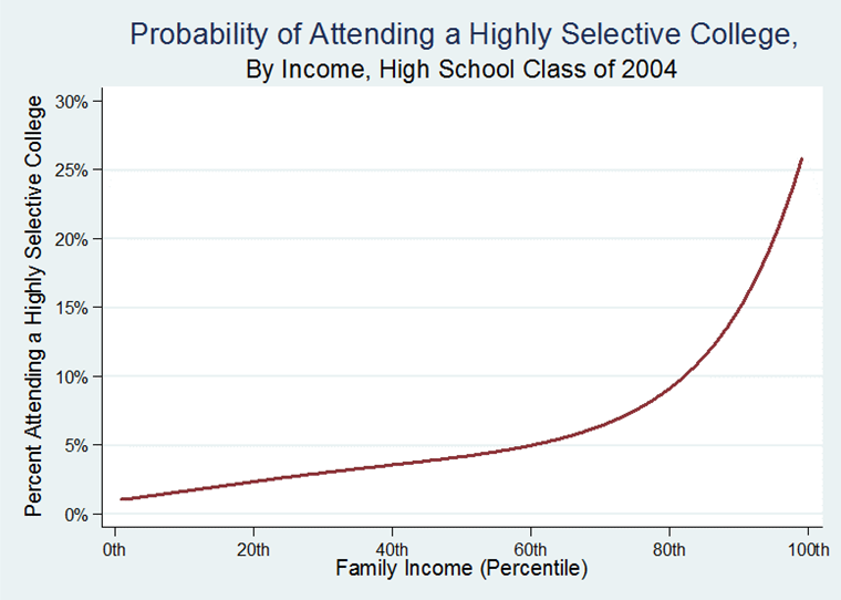
Figure 1. Probability of attending a highly selective college, by income, high school class of 2004. Source: Authors' calculations from ELS:2002. 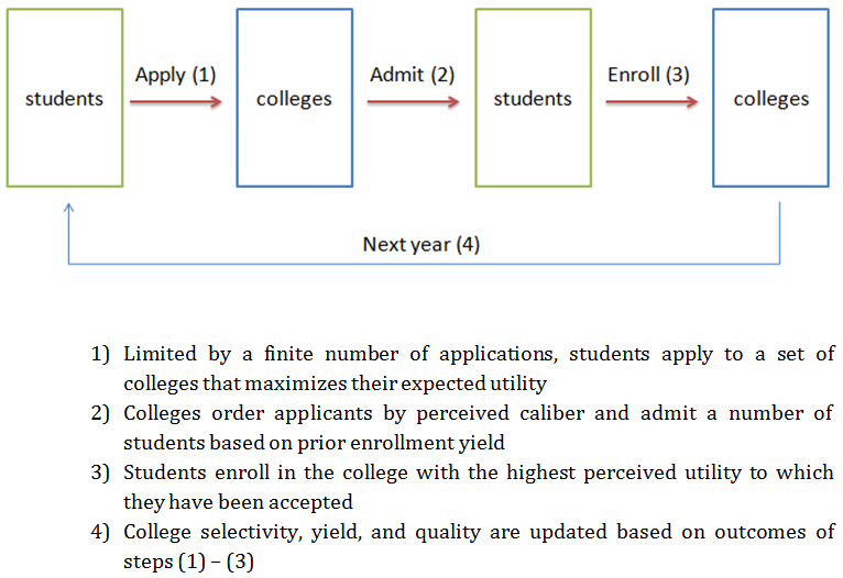
Figure 2. Overview of processes in the agent-based model 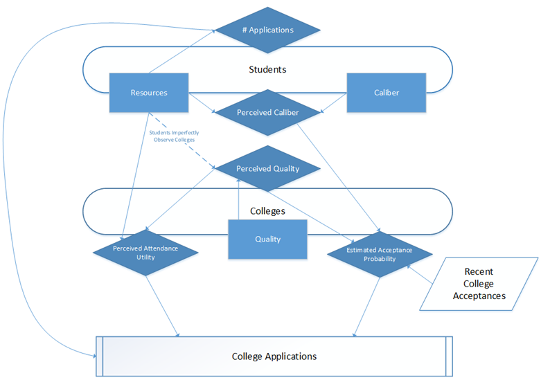
Figure 3. Graphic depiction of the application process in the ABM 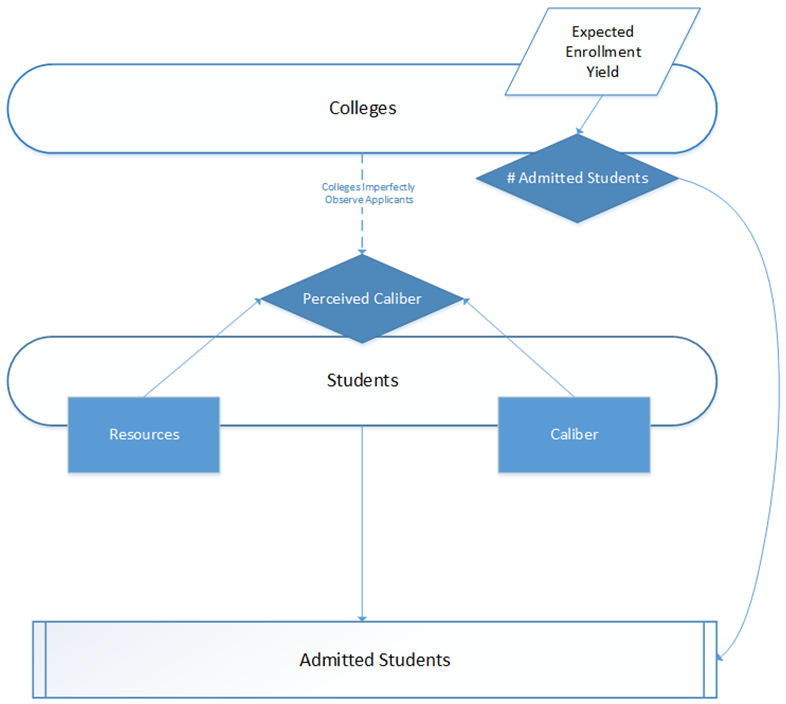
Figure 4. Graphic depiction of the admission process in the ABM 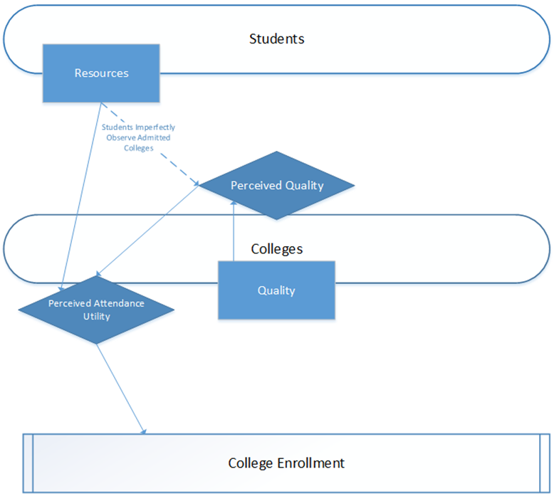
Figure 5. Graphic depiction of the enrollment process in the ABM 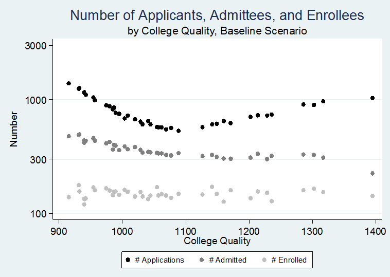
Figure 6. Number of applications, admittees, and enrollees, by college quality, baseline scenario. 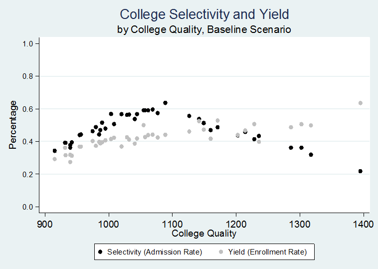
Figure 7. College selectivity and yield, by college quality, baseline scenario. 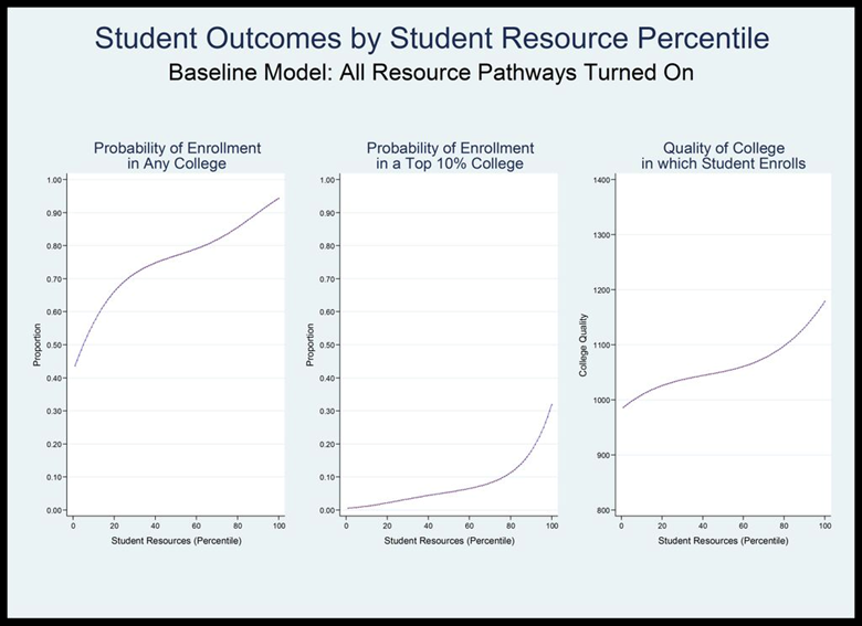
Figure 8. Probability of enrolling in any college, probability of enrolling in a top-10% college and quality of college enrolled in, by student resources percentile, year 30, baseline model. 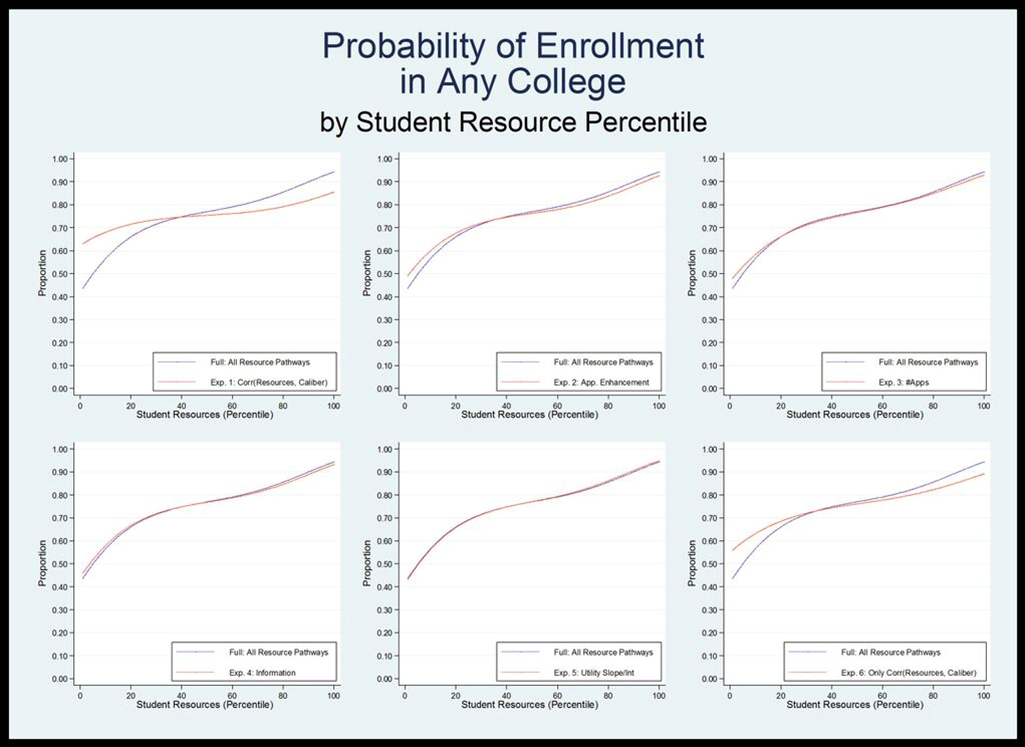
Figure 9. Probability of enrolling in any college, by student resource percentile and resource pathway, year 30. 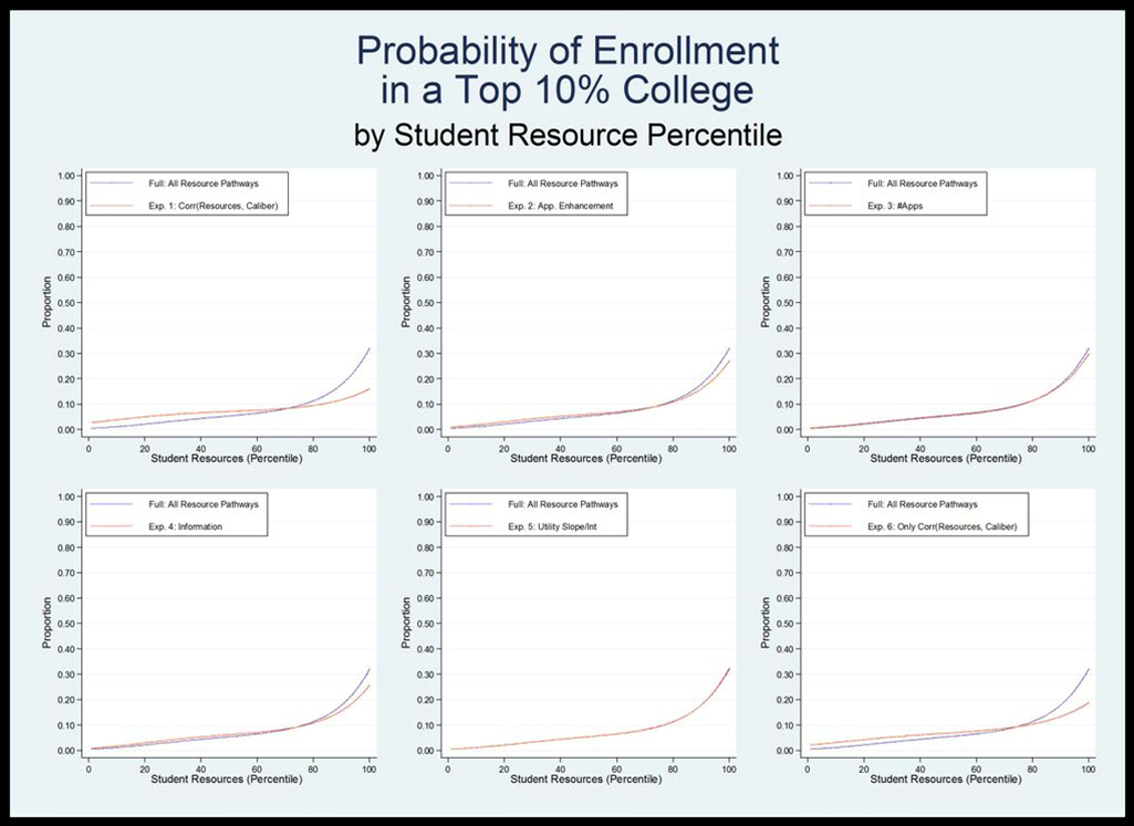
Figure 10. Probability of enrolling in a top-10% college, by student resource percentile and resource pathway, year 30. 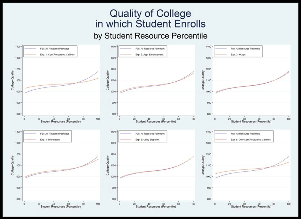
Figure 11. Quality of college enrolled in, by student resource percentile and resource pathway, year 30.
Notes
- 1
Research
from psychology and economics demonstrates
that models of decision making such as this (relying on strict utility
maximization with fully rational actors) are not entirely realistic.
People often exhibit unstable preferences, have inconsistent
preferences over time, and use simplifying heuristics when making
complex decisions (e.g. Simon 1976;
Tversky & Simonson 1993;
Roberts & Lattin 1991;
Swait & Erdem 2007).
We account for this a bit by adding noise to information and
preferences. We don't address the issue of time discounting because the
students in our model have already decided they want to attend college;
they have dealt with the consideration that the returns to college
enrollment are delayed. While a student in our simulation may receive
different returns for attending different colleges, all of the returns
for a given student will be discounted at the same rate.
2 In some ways, using rational decision making in our model provides us with a "best case" scenario. To the extent that real-world students stray from rational decision making, it is likely lower-resource students who stray the most, as they are disadvantaged in part by less access to important college choice information or by constraints on college choices due to finances and mobility. Thus, our rational-choice approach likely understates the stratification our mechanisms contribute to in the real world.
3 The application set selection behavior in our model deviates from selection behavior in the real world. We do this for two reasons. The first is that actual prospective students use a wide variety of different sets of heuristics during the selection process, with actual decision rules both difficult to observe and to satisfyingly quantify. The second is that we believe that there is value in exploring whether, even under simple, "optimal" selection conditions, the resource pathways that we explore can explain observed enrollment patterns. Future models based on this initial, simple model can be constructed to examine the role of more realistic selection behaviors. The algorithm that is used to quickly calculate optimal application portfolios is presented in detail in Appendix D.
4 High school graduates in the U.S. have essentially 3 options – apply to a selective college; apply to a non-selective college (where they are guaranteed admission as long as they meet basic requirements), or don't apply/go to college. Our model simplifies this by eliminating the distinction between selective and non-selective colleges (though the distinction is somewhat murky anyway, since there are minimum requirements even for non-selective schools, so they are in some ways selective, but with a lower bar), and by having all students apply, even those with near 0 chance of admission. In practice, it would matter little if the model didn't allow them to apply since they don't get in/attend
5 By the end of our 30-year model runs, we see stability in college quality values and yield rates as well as student behavior conditional on resources and caliber. Therefore, we believe that focusing on end-run outcomes represents a meaningful analysis of model operation.
6 Many of our parameter estimates come from the Education Longitudinal Study of 2002 (ELS:2002). ELS:2002 is a nationally representative data set collected by The National Center for Education Statistics. It follows 10th grades in 2002 through secondary and postsecondary education and includes high school transcript data, surveys of students and parents, and postsecondary application behavior. We set r to 0.3 in our baseline model, a conservative estimate based on ELS:2002, where the observed correlation between students' SAT scores and the socioeconomic status index is 0.43 (US Department of Education 2006). We set \(b\) to 0.1 based on research that shows that students who take SAT-coaching classes typically raise their SAT scores by approximately 25 points, which is about 12 percent of a standard deviation of SAT scores on the 1600-point SAT scale (Becker 1990; Buchmann et al. 2010; Powers & Rock 1999). We set \(c\) to 0.5 a based on the relationship between the socioeconomic index and the number of schools a student applies to in the ELS:2002 data set (US Department of Education 2006). Finally, we set the ratio of applicants to seats using data from ELS:2002, where the ratio of applicants to seats in very selective colleges (Barrons rankings of 3 or below) is 1.45:1. We tested the sensitivity of our estimates to a range of ratios and found that the number of non-attendees does not drive our results.
7 We were unable to find empirical evidence to guide our selection of several model parameters. Specifically, we were unable to find quantifiable values for the means, minima, and maxima used for the reliabilities with which students perceive their own caliber and college quality; the reliability with which colleges perceive student caliber; and the intercept, \(d\) and \(e\) values used students' evaluation of the utility of attending colleges. However, we attempted to select values that seem sensible: the average student has moderately high, but not perfect, perception of college quality (e.g. familiarity with college rankings) as well as their own caliber (e.g. knowledge of their SAT scores); collectively, college admission officers have quite a bit of experience evaluating students and thus colleges have a highly accurate (but also not perfect) perception of student caliber; and (for example) information and attitudes in their social networks might induce higher-resource students to have a lower evaluation of the utility of attending a low-quality school than their low-resource peers, but also higher evaluations of a high-quality school (Hoxby & Avery 2012). Extensive model testing suggests that our selections of these specific parameter values did not affect the overall interpretation of our results.
8 Like all agent based models, ours is a stylized approximation of individual behavior that is designed to highlight a few key things. In order to fully examine specific facets of this phenomenon (how dynamic processes related to socioeconomic inequality can stratify students among colleges), we have to include simplified models of human behavior. In this case, we have decided to model the relationships between (a) reliability and resources, (b) apparent caliber and resources, and (c) students' evaluation of college utility and resources only as linear relationships (we do not include any higher order polynomials). While a linear relationship seems like a plausible approximation, it's possible that a different functional form would be more appropriate. Our results indicate that these relationships can be important drivers of stratification and future work could explore them in greater depth.
9 Every figure that depicts one of our three main outcomes aggregates all 100 runs, with a line showing a running mean of outcome values by student resource percentiles across runs bounded by a shaded area indicating standard error values.
10 A closer examination of the sets of colleges to which students apply under these different experimental conditions can help to understand these patterns. The figures in Appendix C show the maximum, minimum and mean quality of schools that high and low resource students at all points of the caliber distribution apply to.
Appendix
A
-
Initialization
At the start of each model run, we generate \(J\) colleges with \(m\) available seats per year (for the sake of simplicity, \(m\) is constant across colleges). During each year of the model run, a new cohort of \(N\) students engages in the college application process. Initial college quality (\(Q\)), each student cohort's caliber (\(C\)), and each student cohort's resources (\(R\)) are normally distributed. We allow for a specified correlation between \(C\) and \(R\). The values used for these parameters are specified in Table 1. We select these values to balance computational speed and distribution density as well as to match what we observe from real-world data (ELS:2002).
Submodels
Application. During this stage of our model, students generate an application portfolio, with each student selecting \(n_s\) colleges to which they will apply. Every student observes each college's quality (\(Q_c\)) with some amount of noise (\(u_{cs}\)), which represents both imperfect information and idiosyncratic preferences, and then uses perceived college quality (\(Q_{cs}^\ast\)) to evaluate the potential utility of attendance:
$$ Q_{cs}^\ast = Q_c + u_{cs};\ u_{cs}\sim N(0,\tau_s) $$ (A1) $$ U_{cs}^\ast = a_s + b_s (Q_{cs}^\ast $$ (A2) where \(a_s\) is the intercept of a linear utility function and \(b_s\) is the slope; both intercept and slope may differ between students. Students do not know their own caliber perfectly, but view it with both augmentation and noise:
$$ C_s^\ast = C_s + c_s + e_s;\ e_s\sim N(0,\sigma_s) $$ (A3) where \(c_s\) represents enhancements to caliber that are unrelated to caliber itself (e.g. test preparation, or application essay consultation) and \(e_s\) represents uncertainty. The values that are used for these parameters and their relationships with student resources are listed in Table 1. Based on their noisy observations of their own caliber and college quality, students estimate their probabilities of admission into each college:
$$ P_{cs}= f(C_s^\ast-Q_{cs}^\ast $$ (A4) where \(f\) is a function based on admission patterns over the prior 5 years. In each year \(f\) is estimated by fitting a logit model predicting the observed admissions decisions using the difference between (true) student caliber and college quality for each submitted application over the past 5 years. During the first 5 years of our simulation, the admission probability function has an \(\alpha\) of 0 and a \(\beta\) of −0.015. These values were selected based on observing the admission probability function over a number of model runs; the starting values do not influence the model end-state, but do influence how quickly the function (and the model itself) stabilizes. A student's expected utility of applying to one college is the product of the estimated probability of admission and the estimated utility of attendance.
Students apply to sets of schools that maximize their overall expected utility. For example, if a student chooses to apply to three colleges, then she will select the set of three colleges that they believe has the greatest combined expected utility. In principle, this means that a student agent in the model computes the expected utility associated with applying to every possible combination of three colleges in the model, and then chooses the set that maximizes this expected utility. We develop a fast algorithm, described in Appendix D, that achieves this maximization without requiring the agent to compute and compare all possible application portfolios. The assumption of rational behavior is an abstraction that facilitates focus on the elements of college sorting that we wish to explore. We recognize that real-world students use many different strategies to determine where they apply (e.g. Hoxby & Avery 2012).
Admission. Colleges observe the apparent caliber \((C_s + c_s)\) of applicants with some amount of noise (like the noise with which students view college quality, this also reflects both imperfect information as well as idiosyncratic preferences):
$$ C_{cs}^{\ast\ast} = C_s +c_s + w_{cs};\ w_{cs} \sim N(0,\varphi_s) $$ (A5) Colleges rank applicants according to \(C_{cs}^{\ast\ast}\) and admit the top \(s_c\) applicants. In the first year of our model run, college's expected yield (the proportion of admitted students that a college expects to enroll) is given by:
$$ Yield_c=0.2+.06*College~Quality~Percentile $$ (A6) with the lowest-quality college expecting slightly over 20% of admitted students to enroll and the highest quality college expecting 80% of admitted students to enroll. Colleges thus admit \(m/Yield_c\) students in order to try to fill \(m\) seats. After the first year of a model run, colleges are able to use up to 3 years of enrollment history to determine their expected yield, with \(Yield_c\) representing a running average of the most recent enrollment yield for each college.
Enrollment. Students enroll in the school with the highest estimated utility of attendance (\(U_{cs}^\ast\)) to which they were admitted.
Iteration. Colleges' quality values (\(Q_c\)) are updated based on the incoming class of enrolled students before the next year's cohort of students begins the application process:
$$ Q_c^\prime= 0.9*Q_c +0.1*College~mean~(C_s)$$ (A7) We run our model for 30 years (this appears to be a sufficient length of time for our model to reach a relatively stable state for the parameter specifications that we explore).
Appendix
B
- The following figures are
based on IPEDS
admissions statistics from the
2010–2011 admissions cycle. They were used to help confirm the
calibration of our model. Figures B1
and B2 are intended to be
compared to Figures 3 and 4,
respectively.
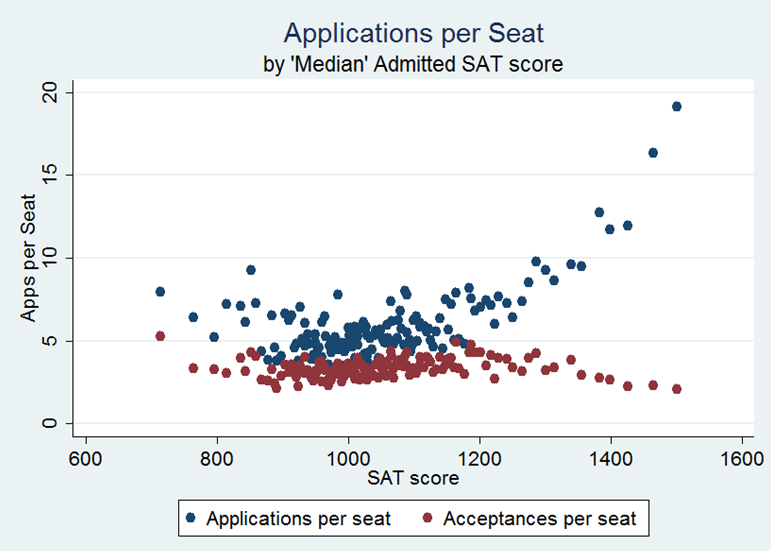
Figure B1. Applications and acceptances per enrolled student, by 'median' admitted SAT score. From IPEDS data from 2010–2011. Median SAT score is approximated usung half of the sum of the 25th and 75th percentile of SAT score. 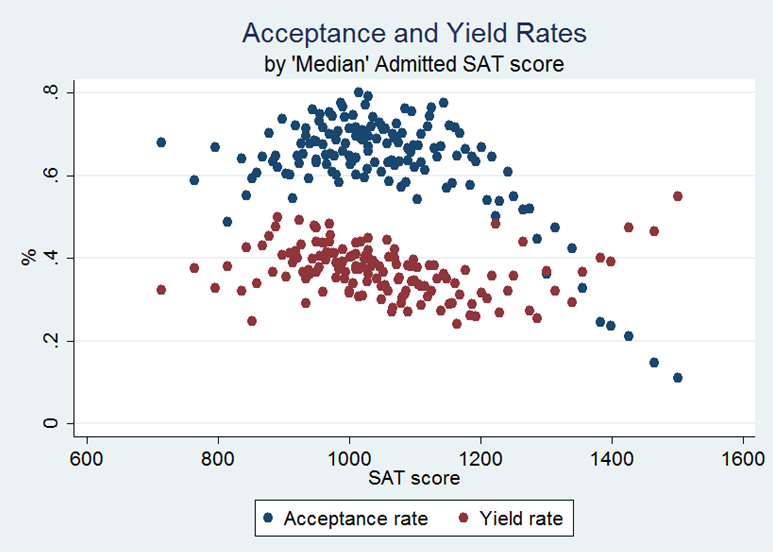
Figure B2. Acceptance and yield rates, by 'median' admitted SAT score. From IPEDS data from 2010–2011Median SAT score is approximated using half of the sum of the 25th and 75th percentile of SAT score
Appendix
C
-
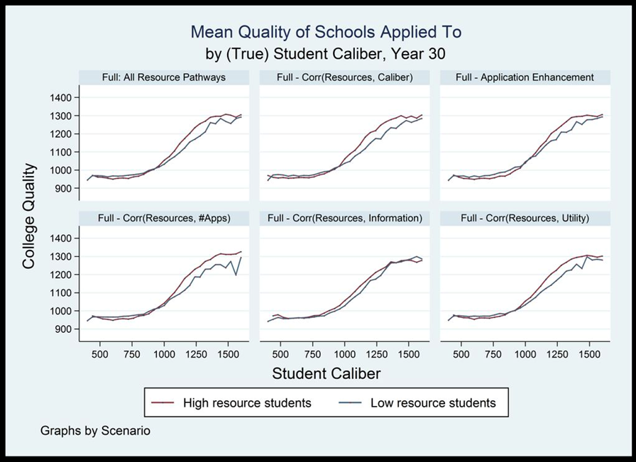
Figure C1. Mean quality of schools applied to, by (true) student caliber and scenario, year 30. Single run. 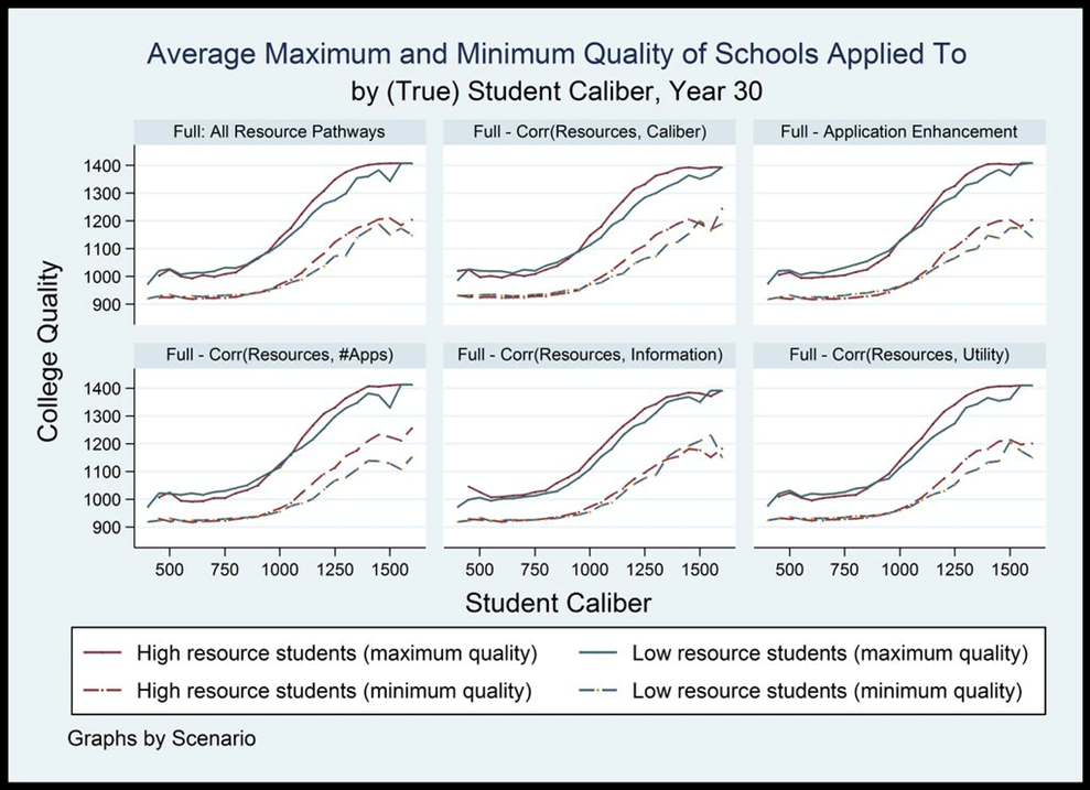
Figure C2. Average maximum and minimum quality of schools applied, by (true) student caliber and scenario, year 30. Single run.
Appendix
D
-
Optimal College Portfolio Algorithm
Notation. Let \(i=1,\ldots,N\) index students and let \(j=1,\ldots,J\) index colleges. Let \(Q_j\) denote the utility of college \(a_j\). Suppose student \(i\) applies to some set \(\mathbf{A}_i=\{a_1,a_2,\ldots,a_n\}\) of \(n\) colleges (where the set is ordered such that \(Q_1< Q_2\cdots< q_n\). Let \(P_{ij}\) indicate the probability that student \(i\) will be admitted to college \(j\), conditional on applying to it. Assume that a student will enroll in the highest utility school to which she is admitted. Denote the utility of this school as \(Q_E\) (and let \(Q_E=0\) if the student is not admitted anywhere).
Now define \(E_i[\mathbf{A}_i]=E[Q_E|\mathbf{A}_i]\). That is, \(E_i[\mathbf{A}_i]\) is the expected value of the quality of the college student \(i\) will enroll in if she is applies to the set of colleges \(\mathbf{A}_i\). Define \(\mathbf{A}_i\backslash a_n = \{a_1,a_2,\ldots, a_{n-1}\}\subset \mathrm{A}_i\); that is, \(\mathbf{A}_i\backslash a_n\) is the subset of \(\mathbf{A}_i\) consisting of all but the college with highest utility. Then \(E_i[\mathbf{A}_i] can be computed recursively as
$$ E_i[\mathbf{A}_i] = P_{in} Q_n + (1-P_{in}) E_i [\mathbf{A}_i\backslash a_n $$ (D1) Now define \(\mathbf{M}_i^n = \{a_1^\ast, \ldots, a_m^\ast\}\) as the set of \(n\) colleges that maximizes \(E_i[\mathbf{A}_i]\). We wish to find this set \(\mathbf{M}_i^n\). Calculating \(E_i[\mathbf{A}_i]\) for all sets \(\mathbf{A}_i\) of size \(n\), however, requires evaluating Equation D1 for \(C_n^J = \frac{J!}{n!(j-n!)}\) possible sets of size \(n\), a prohibitively large number. For example, in our model, where there are \(J=40\) colleges and the typical student applies to 4 colleges, \(C_4^{40} = 91{,}390\); for students applying to 5 or 6 colleges, the numbers are much larger: \(C_5^{40}= 658{,}008\) and \(C_6^{40}=3{,}838{,}380\).
We can find \(\mathbf{M}_i^n\) much more quickly, however. It can be shown that \(\mathbf{M}_i^{n-1}\subset\mathbf{M}_i^n\). That is, the optimal application set of size \(n\) necessarily includes the optimal set of size \(n-1\). This means we can construct \(\mathbf{M}_i^n\) by first identifying \(\mathbf{M}_i^1\), which will contain the college \(a_k\) that maximizes \(E_i[a_k] = P_{ik}Q_k\). Identifying this college requires only \(J\) calculations. Then we can construct the \(J-1\) possible sets that include \(\mathbf{M}_i^1\) plus one additional college. We then find the college \(a_k\) that maximizes
$$ E_i[\{\mathbf{M}_i^1, a_k\}] = P_{ik} Q_k + (1-P_{ik}) E_i [\mathbf{M}_i^1]. $$ (D2) Identifying this college requires \(J-1\) calculations. We then have \(\mathbf{M}_i^2 = \{\mathbf{M}_i^1,a_k\}\). We follow the same process recursively until we have identified \(\mathbf{M}_i^n\), a process that will take only \(\sum_{m=0}^{n-1} (J-m) = n\left(J-\frac{(n-1)}{2}\right)\) calculations. For example, in our model, where there are \(J=40\) colleges, students choosing the optimal sets of 4, 5, or 6 colleges will have to make 154, 190, or 225 calculations under our algorithm, respectively. The recursive algorithm is orders of magnitude faster than the brute force algorithm in this case.
References
- ALON,
S. (2009). The evolution of class inequality in higher education:
Competition, exclusion, and adaptation. American Sociological
Review, 74, 731–755. [doi:10.1177/000312240907400503]
ASTIN, A., & Oseguera, L. (2004). The declining "equity" of American higher education. The Review of Higher Education, 27, 3, 321–341. [doi:10.1353/rhe.2004.0001]
AVERY, C., & Kane, T. (2004). Student perceptions of college opportunities: The Boston COACH Program. In C. Hoxby (Ed.), College choices: The economics of where to go, when to go, and how to pay for it (pp. 355–391). Chicago: University of Chicago Press. [doi:10.7208/chicago/9780226355375.003.0009]
BAILEY, M. J., & Dynarski, S. M. (2011) Inequality in postsecondary education. In Duncan, G. C. & Murnane, R. (Eds.) Whither Opportunity? (pp. 117–132). New York: Russell Sage Foundation.
BASTEDO, M. N., & Jaquette, O. (2011). Running in place: Low-income students and the dynamics of higher education stratification. Educational Evaluation and Policy Analysis, 33, 3, 318–339. [doi:10.3102/0162373711406718]
BECKER, B. J. (1990). Coaching for the Scholastic Aptitude Test: Further synthesis and appraisal. Review of Educational Research, 60, 373–417. [doi:10.3102/00346543060003373]
BELLEY, P., & Lochner, L. (2007). The changing role of family income and ability in determining educational achievement. Journal of Human Capital, 1, 1, 37–89. [doi:10.1086/524674]
BLACK, D., & Smith, J. (2004). How robust is the evidence on the effects of college quality? Evidence from matching. Journal of Econometrics, 121, 99–124. [doi:10.1016/j.jeconom.2003.10.006]
BOUDON, R. (1974). Education, Opportunity, and Social Inequality: Changing Prospects in Western Society. New York: John Wiley & Sons.
BOWEN, W. G., Chingos, M. M., & McPherson, M. S. (2009). Crossing the Finish Line: Completing College at America's Public Universities. Princeton: Princeton University Press.
BREEN, R., & Goldthorpe, J. H. (1997). Explaining educational differentials: Towards a formal rational action theory. Rationality and Society, 9, 3, 275–305. [doi:10.1177/104346397009003002]
BREEN, R., van de Werfhorst, H. G., & Jaeger, M. M. (2014). Deciding under doubt: A theory of risk aversion, time discounting preferences, and educational decision-making. European Sociological Review, 30, 2, 258–270. [doi:10.1093/esr/jcu039]
BRUCH, E., & Atwood, J. (2012). Agent-based models in empirical social research. Working paper.
BUCHMANN, C., Condron, D. J., & Roscigno, V. J. (2010). Shadow education, American style: Test preparation, the SAT and college enrollment. Social Forces, 89, 2, 435–461. [doi:10.1353/sof.2010.0105]
CABRERA, A. F,. & La Nasa, S. M. (2000). Understanding the college-choice process, New Directions for Institutional Research, 107, 5–22. [doi:10.1002/ir.10701]
DALE, S., & Krueger, A. B., (2011). Estimating the return to college selectivity over the career using administrative earnings data. National Bureau of Economic Research Working Paper No. 17159.
DIMAGGIO, P. & Garip, F. (2012). Network effects and social inequality. Annual Review of Sociology, 38, 93–118 [doi:10.1146/annurev.soc.012809.102545]
GRODSKY, E., & Jones, M. T. (2007). Real and imagined barriers to college entry: Perceptions of cost. Social Science Research, 36, 2, 745–766. [doi:10.1016/j.ssresearch.2006.05.001]
HENRICKSON, L. (2002). Old wine in a new wineskin: College choice, college access using agent-based modeling. Social Science Computer Review, 20, 400–419. [doi:10.1177/089443902237319]
HOEKSTRA, M. (2009) The effect of attending the flagship state university on earnings: a discontinuity-based approach. The Review of Economics and Statistics, 91, 4, 717–724. [doi:10.1162/rest.91.4.717]
HOWELL, J. S. (2010). Assessing the impact of eliminating affirmative action in higher education. Journal of Labor Economics, 28, 1, 113–166. [doi:10.1086/648415]
HOXBY, C. M., & Avery, C. (2012). The missing "one-offs": The hidden supply of high-achieving, low income students. National Bureau of Economic Research Working Paper No. 18586.
HOXBY, C. M., & Turner, S. (2013). Expanding college opportunities for low-income, high-achieving students. Stanford Institute for Economic Policy Research Discussion Paper No. 12-014.
KAREN, D. (2002). Changes in access to higher education in the United States: 1980-1992. Sociology of Education, 75, 3, 191–210. [doi:10.2307/3090265]
LONG, M. C. (2008). College quality and early adult outcomes. Economics of Education Review, 27, 588–602. [doi:10.1016/j.econedurev.2007.04.004]
MANZO, G. (2013). Educational choices and social interactions: A formal model and a computational test. Comparative Social Research, 30, 47–100. [doi:10.1108/S0195-6310(2013)0000030007]
MAROULIS, S., Guimerà, R., Petry, H., Stringer, M. J., Gomez, L. M., Amaral, L. A. N., & Wilensky, U. (2010). Complex systems view of educational policy research. Science (Washington), 330, 6000, 38–39. [doi:10.1126/science.1195153]
MCDONOUGH, P. M. (1997). Choosing Colleges: How Social Class and Schools Structure Opportunity. Albany: State University of New York Press.
POWERS, D. E., & Rock, D. A. (1999). Effects of coaching on SAT I: Reasoning test scores. Journal of Educational Measurement, 36, 2, 93–118. [doi:10.1111/j.1745-3984.1999.tb00549.x]
REARDON, S. F. (2011). The widening academic achievement gap between the rich and the poor: New evidence and possible explanations. In Duncan, G.C. & Murnane, R. (Eds.) Whither Opportunity? New York: Russell Sage Foundation.
REARDON, S. F., Baker, R., B., & Klasik, D. (2012). Race, income, and enrollment patterns in highly selective colleges, 1982–2004. Center for Education Policy Analysis.
ROBERTS, J. H., & Lattin, J. M. (1991). Development and testing of a model of consideration set composition. Journal of Marketing Research, 429–440. [doi:10.2307/3172783]
RODERICK, M., Nagaoka, J., Coca. V., & Moeller, E. (2008). From high school to the future: Potholes on the road to college. Chicago: Consortium on Chicago School Research at the University of Chicago.
RODERICK, M., Nagaoka, J., Coca. V., & Moeller, E. (2009). From high school to the future: Making hard work pay off. Chicago: Consortium on Chicago School Research at the University of Chicago.
SEGOVIA-JUAREZ, J. L., Ganguli, S., & Kirschner, D. (2004). Identifying control mechanisms of granuloma formation during M. tuberculosis infection using an agent-based model. Journal of Theoretical Biology, 231, 3, 357–376. [doi:10.1016/j.jtbi.2004.06.031]
SIMON, H. (1976). Administrative Behavior. New York, NY: The Free Press.
SMITH, J. (2013). The Effect of College Applications on Enrollment. The B.E. Journal of Economic Analysis & Policy, 14, 1, 151-188. [doi:10.1515/bejeap-2013-0002]
SWAIT, J., & Erdem, T. (2007). Brand effects on choice and choice set formation under uncertainty. Marketing Science, 26, 5, 679–697. [doi:10.1287/mksc.1060.0260]
TVERSKY, A. & Simonson, I. (1993). Context-Dependent Preferences. Management Sciences, 39, 10, 1179–1189. [doi:10.1287/mnsc.39.10.1179]
US DEPARTMENT OF EDUCATION (2006). National Center for Education Statistics. Education Longitudinal Study (ELS), 2002 and 2006: Base Year through Second Follow-up.