Degrees of Separation, Social Learning, and the Evolution of Cooperation in a Small-World Network

Hide
Article Tools

Smaller Text Bigger

Bookmark:

Export citation

Articles with the same author(s)

Articles with similar keywords

Articles citing this article

Download this article in PDF format

Alert me when this article is cited within JASSS

Send a link to this article to a colleague

Abstract

: We analyze a novel agent-based model of a social network in which agents make contributions to others conditional upon the social distance, which we measure in terms of the “degrees of separation” between the two players. On the basis of a simple imitation model, the emerging strategy profile is characterized by high levels of cooperation with those who are directly connected to the agent and lower but positive levels of cooperation with those who are indirectly connected to the agent. Increasing maximum interaction distance decreases cooperation with close neighbors but increases cooperation with distant neighbors for a net negative effect. On the other hand, allowing agents to learn and imitate socially distant neighbors increases cooperation for all types of interaction. Combining greater interaction distance with greater learning distance leads to a positive change in the total social welfare produced by the agents’ contributions.
Keywords:: Cooperation, Social Networks, Small-World, Modern Society, Simulation, Agent-Based

Introduction

1.1

Cooperation is a fundamental mechanism of all social life, and is, therefore, at the core of social science (Axelrod & Hamilton 1981; Ostrom 1998). Thomas Hobbes speculated that absent some common power capable of compelling tolerance of one another, the constant pain of privation will drive individuals to lie, cheat, steal, and bludgeon for a moment's respite: "Hereby it is manifest, that during the time men live without a common Power to keep them all in awe, they are in that condition which is called Warre; and such a warre, as is of every man, against every man" (Hobbes 1969). Accordingly, he concludes that the advent of such a power, or a Leviathan, was a prerequisite for and thus the basis of all society.

1.2

Once strictly the purview of philosophy, the problem of cooperation has perplexed life scientists since Charles Darwin first elaborated on the principles of the origins of species through natural selection (Darwin 2007). In an influential paper, West et al. (2007, p. 416) defined cooperation as "a behaviour which provides a benefit to another individual (recipient), and which is selected for because of its beneficial effect on the recipient" . This definition seemingly contradicts the theory of evolution by natural selection because, all things equal, such an act should reduce the relative fitness of the cooperator and, therefore, be selected against in favor of more "selfish genes" (Dawkins 1976). Mutual defection, however, is not a foregone conclusion. According to Elinor Ostrom, diverse and decentralized norms in the form of cultural institutions may emerge to prevent resource exhaustion (Ostrom 1990). For comprehensive summaries of the major explanations of evolution of cooperation see Nowak (2006) and Zaggl (2014).

1.3

Our present focus is on evolution of cooperation within a small-world social network model (Watts & Strogatz 1998). Population structures have been known to promote cooperative behavior by means of cooperative clustering and assortative interactions (Epstein 1998; Fu et al. 2007; Jun & Sethi 2007; Kuperman & Risau-Gusman 2012; Lindgren & Nordahl 1994; Macy & Skvoretz 1998; Ohtsuki et al. 2006; Shutters & Hales 2013; Spector & Klein 2006; Xianyu 2012). Our novel contribution is to introduce a realistic—yet previously unexplored—model of cooperation conditional upon the social distance between the agent and others. In our unweighted social network, this social distance can be measured by means of the degrees of separation, defined here as the number of connections (edges) between any two agents (nodes). For example, two people who know each other are separated by one degree. Two people who do not know each other but have a common acquaintance are separated by two degrees, and so on.

1.4

A number of existing models examine the relationship between cooperation and the interaction or neighborhood radius (Jun & Sethi 2007; Shutters & Hales 2013; Spector & Klein 2006). The models show that, in the ring network, increasing the interaction/neighborhood radius decreases cooperation. Notice that according to these approaches, once a neighborhood radius is defined agents do not discriminate between the game partners on the basis of their social distance with that distance (that is, the number of nodes separating them). Introducing strategies conditional upon the social distance is our main contribution and an importance substantive difference between our model and the above approaches. Moreover, we also introduce a "learning distance" parameter which is a measure—separate from interaction distance—of how far an agent looks in order to imitate the payoff-increasing strategies of agents (see below for details).

1.5

Further notice the difference between (a) the strategies conditional upon social distance, and (b) the strategies conditional upon the expectations or the actual behavior of game partner's (Szolnoki & Perc 2012; Xianyu 2012). In the latter case, the idea behind conditional cooperation is based upon the Tit-for-Tat strategy (Axelrod & Hamilton 1981): cooperate if you expect the partner to cooperate, otherwise defect. Cooperation conditional upon social distance allows agents to choose different strategies depending on the degrees of the separation between the game partners.

1.6

To our knowledge, two existing models overlap with our approach the most. Lei et al. (2010) present a model based upon the heterogeneous allocation of funds, in which the size of the contributions is based on the "link weight". Such heterogeneity appears to promote cooperation; however, the interactions occur only between the direct neighbors. In another paper, Chiang proposes cooperative strategies, conditional on the structural attributes of the nodes occupied by actors such as node degree, clustering coefficient, betweenness, and the eigenvector centrality (Chiang 2013). The main result of the paper is that strategies that command one to cooperate with neighbors with either higher or lower nodal attributes are advantageous (Chiang 2013, section 3.1). The result, while interesting, is not easy to interpret substantively. Similarly, it is not obvious how and why the selected network characteristics should matter for a decision whether or not to cooperate with the other player. On the other hand, our approach based on the degrees of separation has a natural and intuitive interpretation: people may be more cooperative with those who are socially close to them.

1.7

We also emphasize that the present model makes no assumptions about genetic relatedness between agents, faculties of memory necessary for either direct or indirect reciprocity, punishment, or group identification allowing for multilevel selection. Further, we do not assume agents alter network structure by disconnecting from defectors (Fu et al. 2007). Agents also do not inherit payoffs from the previous time periods as in Liu et al. (2010a, 2010b). In other words, we offer a minimalist model that is sufficient to explain the evolution of cooperation in a society without using the conventional approaches (Nowak 2006; Zaggl 2014).

1.8

Our goal is two-fold: (a) to model the evolution of cooperation in society, and (b) to examine how cooperation is affected by social distances. Specifically, we study if cooperation propensities are different for interactions with the first, second, third, and fourth degree neighbors. We further explore how the parameters of the computational model and network characteristics affect the behavior. Our research questions include the following:

Does cooperation with strangers come at the cost of cooperation with close neighbors?
Does learning from strangers lead to higher or lower rates of cooperation?
What are the effects of greater interaction and greater learning distances on the accumulated social wealth?
Which social network characteristics improve the prospects of cooperation with the first degree neighbors, second degree neighbors, and so on?

Degrees of Separation and Conditional Cooperation

2.1: In a basic model of cooperation on a social network, individuals interact with their immediate neighbors given the players' types, histories of interaction, reputations, or arbitrary tags. Following the interaction, individuals update their behavior by looking at the payoffs of their immediate neighbors. Although there are many different assumptions with respect to agents' characteristics, behavior, and the rules of the game in general, all existing models—to our knowledge—make the same underlying assumption: local interaction and learning/reproduction are characterized by one degree of separation. While we believe in the idea of local interaction and learning, we do not want to restrict locality to the one degree of separation.
2.2: In the modern world, for instance, we often interact with individuals who are not immediately connected to us. Some of the strangers may be socially close to us (e.g., two degrees of separation); others may be relatively more distant (e.g., three or more degrees of separation). Similarly, it is also possible that we may learn something from strangers, that is, imitate their behavior if we find it attractive. In the real world, the social distance is likely a function of similarity of individual attributes, such as occupation, residence, race and ethnicity, age, income, education, and so on. In the social network model, the social distance is represented by the degrees of separation, which may be considered as a summary of the totality of individual attributes mentioned above. Importantly, much of these attributes are outwardly visible or otherwise detectable (as in manner of speech, dress, symbolic ornamentation, etc). Such "ethnic markers" (Boyd & Richerson 1987) allow for fast and efficient identification of strangers in terms of group memberships and affiliations. With a glance, individuals are thus able to ascertain an actionable approximation of a strangers' social distance and engage preset behavioral strategies during an encounter. We acknowledge that the notion of social distance is much more complicated and nuanced in the real world than in a computational model, which is always a simplification of reality. Nevertheless, we believe that the number of degrees of separation, at the aggregate level, is a useful approximation of the social distance.
2.3: Some readers accustomed to social network analysis may ask: "If an agent interacts with someone at social distance three, isn't their social distance updated to one since they had a direct interaction?" We do not assume this in our model. Rather, in our model degrees of separation may be better understood as ordinal categories ordered along some dimension of social similarity. Within a large population center, as in a city, individuals do not just interact with a fixed number of people. They interact with hundreds of other individuals sometimes on a daily basis, many of whom shall never be encountered again. Naturally, such encounters do not automatically make the latter their "close friends." However, we maintain that despite the pervasiveness of encounters with unknown individuals, ubiquitous cultural and ethnic markers allow individuals to identify others, if not as individuals, but in terms of broad social categories. Further, we hold that individuals perceive such categories along a dimension of social distance, relative to them personally, which are reasonably represented as degrees of separation. This, in turn, is what allows them to engage behavioral strategies assuming a certain degree of familiarity, even when none truly exists.
2.4: Thus, the main difference between our model and other models of cooperation on a social network is the fact that agents can interact and learn from strangers (two or more degrees of separation). There are four major consequences of this modeling approach.
2.5: First, individuals in the model may have different probabilities of cooperation for different degrees of separation. Therefore, each individual needs a vector of cooperation probabilities as opposed to a single value.
2.6: Second, we need to decide how often the individuals in the network interact with the first, second, third, and fourth degree neighbors. We assume that each agent randomly chooses a social distance; then the agent randomly chooses a game partner given the social distance. In the real world, an individual is more likely to interact with a first degree neighbor than a fourth degree neighbor. On any small-world network with a rewiring factor greater than 0.0 (i.e., a "broken" ring), the number of nodes at distance d is increasing in d. Accordingly, our random matching algorithm reproduces this phenomenon since any given individual at higher degrees of social distance is rendered less likely to be chosen than any given individual at lower degrees of distance. Thus, while agents interact with more closely related individuals more frequently than more distantly related individuals, the total number of interactions with first degree neighbors and fourth degree neighbors will be the same by construction, given our assumptions. This is especially important for us since we want to compare cooperation propensities for the different degrees of separation for the same frequency of interactions, i.e., without making first degree cooperation potentially more appealing.
2.7: Third, we need a simple yet plausible model of social learning. We chose a model, in which individuals imitate behavior of the individual with the highest payoff. This is a simple, conservative assumption that has already been used by other scholars (Helbing & Yu 2009), which is known to favor defection (Ohtsuki et al. 2006).
2.8: Finally, we need to examine a larger parameter space than in the model characterized by a binary choice (cooperate or defect) and interaction with immediate neighbors. In the latter case, the choice of a parameter interval is guided by a goal to find a threshold value in the interval that would affect the agents' cooperative behavior. In our model, agents may have four different probabilities of cooperation for each social distance (one, two, three, and four degrees of separation), thus, potentially requiring four separate threshold values and much larger parameter interval.

Agent-Based Model

3.1

In recent years agent-based modeling has becoming increasingly recognized as a useful tool for generating insights into complex sociological phenomena (Eguíluz et al. 2005; Hedström & Ylikoski 2010; Macy & Skvoretz 1998). This is in large part due to the unique capability simulations provide us to glimpse the emergence of macro-level patterns from micro-level foundations in interpersonal interaction. To examine conditional cooperation for a large set of parameters we create an agent-based computational model and conduct multiple simulation runs. The model is based on a population of N agents which form a social network such as the small-world network (Watts & Strogatz 1998). To construct the small-world network, it is necessary to place N agents (nodes) on a circle, add k connections (edges) to the closest neighbors, and rewire some of the close connections to random agents in the network depending on the rewiring probability p. Thus, any small-world network is created as a graph G[N, k, p]. For each simulation run, the social network parameters are drawn from a uniform probability distribution.

3.2

Each agent \(i\) is given a conditional strategy \(S\) defined as \(S(i)[P(d)]\), where \(P(d)\) is a vector describing \(i\)'s propensity to cooperate with its neighbors separated by (\(1, \ldots, d\)) degrees of separation. The number of elements in the vector is equal to the exogenous interaction distance (\(ID\)). For example, for \(ID = 2\), the strategy profile is \(S(i)[p(1), p(2)]\). The initial propensity to cooperate for all types of neighbors is drawn randomly from the uniform probability distribution \(U[0, 1]\).

3.3

For t generations, agents interact with each other in a continuous Prisoner's Dilemma game. Agents' matching is determined probabilistically by first randomly choosing a "social distance" \(d\) and then randomly choosing an available partner, given \(d\). Notice that since the number of neighbors is increasing in \(d\), this matching rule implies more frequent interactions with any given neighbor at lower social distances than higher. The payoff to an agent \(i\) interacting with agent \(j\) is defined as \(U(i, j) = b*S(j)[d]- c*S(i)[d]\), where \(b\) and \(c\) are the benefit and cost of cooperation (\(b>c\)), and \(S(i)[d]\) and \(S(j)[d]\) are the agents \(i\)'s and \(j\)'s propensities to cooperate with a neighbor separated from them by \(d\) degrees of separation. Notice that \(d\) is always the same for both agents since it is the number of degrees of separation between them.

3.4

At the end of each generation, agents evaluate the relative success of their strategies by comparing their own payoffs to the payoffs of other agents in their vicinity, the radius of which is equal to their learning distance. We acknowledge the recent contributions of Wang et al. (2013), whose innovative model of imitation demonstrates that cooperation increases if agents are allowed to take into account payoffs to other individuals' neighbors. The mechanism by which this appears to work seems to be a built-in bias, disposing agents to imitate the strategies of agents embedded in cooperative clusters. This may, in fact, be a plausible supposition. However, we maintain that the standard approach—i.e., that agents appraise others' fitness levels based solely on their own payoffs—makes a harder, more vetted test of our hypotheses.

3.5

In addition to imitation, agent strategy profiles are also subject to random mutation. Random mutation is rare in our simulation, as in nature, however even small mutation rates are sufficient to prevent model convergence on local minima. In this model, mutation rate mut is a random parameter in \([0, 0.005]\). Each time period with probability mut an agent's strategy profile is regenerated according to the same initial probability distribution.

3.6

Table 1 provides a detailed description of a single run of the computer model. The actual "ready-to-run" Python code is presented in the Appendix.

Table 1: Agent-based model. Structure of the model.

1. Define simulation parameters
         T                - number of time periods in one run
         degs           - maximum possible interaction distance
         maxlearn   - learning distance
         N                - number of agents in the network
         K                - average number of neighbors in the network
         P                - rewiring probability
         R                - number of games per individual per time period
         SF              - starting fitness
         Cmin         - initial contribution minimum
         Cmax         - initial contribution maximum
         c                - cost of cooperation, to self
         b                - benefit of cooperation, to the other
         mut            - mutation rate

2. Create arrays to store population data: pop (current time period), pop2 (next time period).
First column (pop[:,0]) stores fitness values for each individual
Subsequent columns (pop[:,1:]) store contribution strategies for each degree of separation

3. Generate starting fitness and initial contribution strategies given degs, Cmin, and Cmax

4. Create small world network given N, K, and P

5. Generate three dimensional array popD describing neighborhood structure:
         - dimension 1: degree of separation (degs)
         - dimension 2: agents in the network (N)
         - dimension 3: index values of the neighbors for a given degree of separation

6. Model interactions, given T and R:
         - for each individual i, randomly choose a degree of interaction rdeg
         - given rdeg, choose a random partner j from the list of possible partners in popD
         - update players payoffs given i's and j's strategies for their degree of separation, saving the payoffs to pop2

7. Model imitation for each individual i assigning values to pop2 (next generation strategies):
         - if mutation takes places (mutation probability is mut), generate a completely new random set of strategies for the individual
         - in the absence of mutation, examine all neighbors of the individual, given maxlearn
         - imitate the strategy of the neighbor with the highest payoff/fitness

8. Reset fitness of all individual given SF

9. Assign next generation values pop2 to the current population data matrix pop

10. Save data into data array and proceed to the next time period

11. Generate figures and save data to a file

Results

Illustrative examples

4.1

In this section, we provide several examples to illustrate our results; each example is based on the average of 100 runs for a chosen set of parameters. The following parameters were held constant: \(N=400\), \(K=4\), \(P=0.1\), \(R=1\), \(SF=0\), \(Cmin=0\), \(Cmax=1\), \(c=1\), \(mut = 0.001\). Our primary focus was to examine contribution behavior for benefits of cooperation \(b\), and interaction (\(ID\)) and learning (\(LD\)) distances. In the following section, we present a more systematic examination of the parameter space and other variables based on Monte Carlo experiments and regression analysis of 30,000 simulation runs.

4.2

First, we use our model restricting both interaction and learning distance to one degree of separation. As expected (Nowak 2006; Ohtsuki et al. 2006), the benefit of cooperation \(b\) determines if the cooperative behavior is selected (Figure 1). Specifically, for a small-world network with 4 neighbors (\(K=4\)) and the rewiring probability \(P=0.1\), average contributions converge to 0.0 for \(b=2\), 0.42 for \(b=3\), 0.70 for \(b=4\), and 0.88 for \(b=6\).

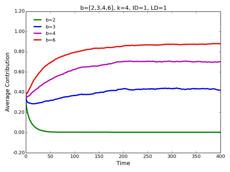
Figure 1. Average contributions for different benefits of cooperation in a basic model.

4.3

Our main interest is to examine how contribution behavior may change if we allow agents to interact with and learn from distant neighbors. Our most immediate finding is based on the fact the conditional strategies lead to robust evolution of [conditional] cooperation (Figures 2 and 3). While the agents contribute most to the immediate neighbors (one degree of separation), the contributions decrease for the neighbors who are separated by two or more degrees. Notably, contributions to the second degree neighbors are consistently greater than contributions to the third degree neighbors; contributions to the third degree neighbors are greater than contributions to the fourth degree neighbors, and so on.

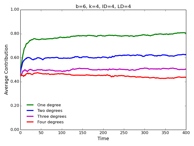
Figure 2. Average contributions for high benefit of cooperation, and high interaction and learning distances.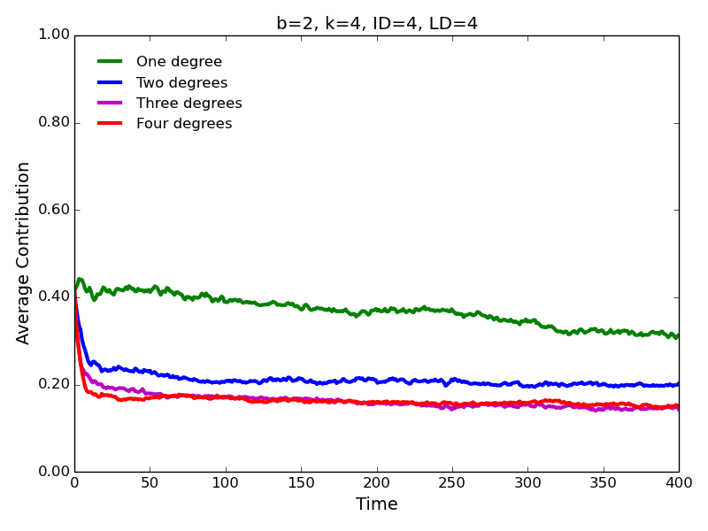

Figure 3. Average contributions for low benefit of cooperation, and high interaction and learning distances.

4.4

The same pattern is observed for the high (\(b=6\)) and low (\(b=2\)) benefits of cooperation. Not surprisingly, the levels of cooperation are lower in the latter case. Surprising is the fact that, contrary to the approach characterized by ID=1 and LD=1 (Figure 1), we observe substantial levels of cooperation for \(b=2\), especially, for the interaction with the immediate neighbors. Notice that cooperation evolves despite the fact that \(b/c < k\) (\(2/1 < 4\)), i.e., contrary to the simple rule for the evolution of cooperation (Nowak 2006; Ohtsuki et al. 2006).

4.5

Increasing interaction distance leads to a slightly lower contributions to the first degree neighbors (Figure 4) and slightly higher contributions to the second and third degree neighbors (Figure 5)—we confirm these results for a larger parameter space in the section below.

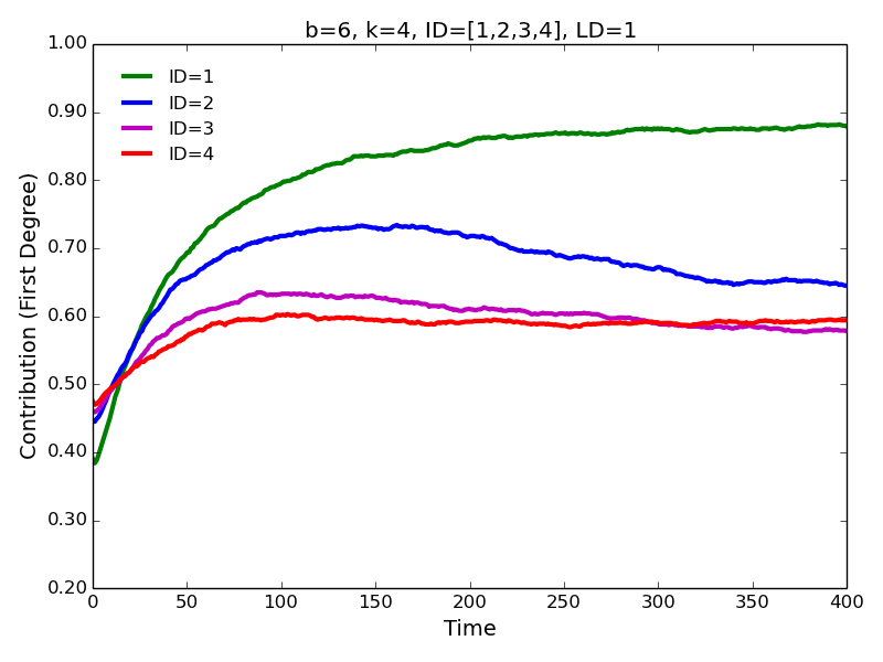
Figure 4. First degree contributions for different values of interaction distance.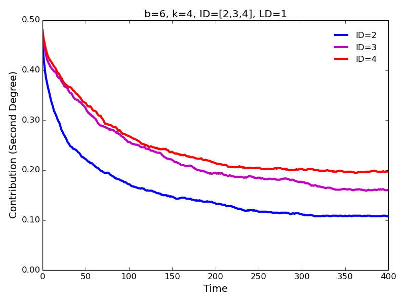

Figure 5. Second degree contributions for different values of interaction distance.

4.6

On the other hand, increasing learning distance has a large positive effect on contributions to all types of neighbors (using Monte Carlo experiments we confirm this finding as well). The most dramatic increase in cooperation is observed for when learning distance is increased from 1 to 2. The magnitude of the impact appears to be comparable for the first and second degree contributions.

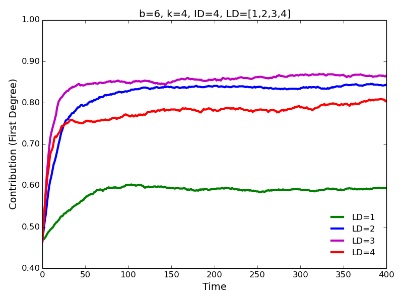
Figure 6. First degree contributions for different values of learning distance.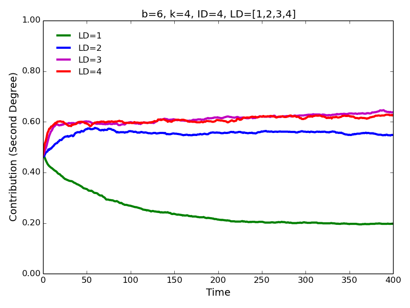

Figure 7. Second degree contributions for different values of learning distance

4.7

In the following section we examine these and other results using a larger parameter space by means of Monte Carlo experiments and a more systematic approach by means of regression analysis. We also offer substantive explanations behind our findings.

Monte Carlo experiments

4.8

To examine the relationship between the parameters of the model and the emerging levels of conditional cooperation, we conducted 30,000 simulations. Each simulation lasted 1,000 time periods to ensure convergence (in most cases, convergence occurred between 100 and 400 time periods). Notice that in the presence of mutation, complete convergence of strategies was not possible.

4.9

Interaction distance (\(ID\)) was drawn randomly from a uniform discrete distribution \([1, 4]\). 10,000 runs were conducted for learning distance \(LD = 1\); 10,000 for \(LD = 2\), and 10,000 for \(LD = 3\). Other simulation parameters were chosen randomly from a parameter space large enough to obtain a large variance in behavior (i.e., different values of contributions for all possible degrees of separation).

4.10

In generating Watts-Strogatz random graphs, it is necessary to specify the parameter \(k\), representing the number of direct connections to other agents, or edges, each node possesses. Parameter \(k\) is supported by the discrete set [2, 4, 6].

4.11

Another factor to take into account is that due to random rewiring, it is possible for some Watts-Strogatz random graphs to be disconnected; i.e., to have multiple connected components. This probability is increasing in the probability of rewiring \(p\), and decreasing in the number of connections per node \(k\). To keep account of this during the Monte Carlo simulation, we store a value (componqty) representing the number of connected components in the output data file. In 24,168 of 30,000 cases (80.6%), our random networks contained only a single connected component. In 3,553 cases (11.9%) of the remaining cases there were exactly two connected components, and in 1,628 cases (5.4%) there were exactly three. In 651 cases (2%) there were more than 3 connected components. While we observe a small but significant correlation between first-degree cooperation and componqty (\(-0.07\), \(p < 0.001\)), the correlations between componqty second, third, and fourth degree cooperation were not significantly different from zero. It is important to keep in mind, however, that insofar as these effects are interesting, they are interesting because they are expressions of the parameters \(p\) and \(k\). It is also important to note that the presence of multiple connected components does not change the mechanics of the simulation. Rather, in cases of multiple connected components we are merely observing smaller networks. Since the data vector population size only records the global population \(n\), this coefficient could be biased downwards. This is, in fact, what we observe. Not including componqty in the regression model reduces the coefficient on population size from 0.00616 to 0.00574. However and again, insofar as this result is interesting, it is because these are the effects of \(k\) and \(p\) (i.e., few connections and greater rewiring produce smaller connected networks).

4.12

In light of these considerations, we do not include componqty in our regression model. This leaves the interpretations of population size \(n\), \(k\) and \(p\) as straightforward as possible, while also promoting parsimony since there remains only exogenous parameters of the simulation on the right-hand side of the equation.

Average propensity to cooperate and social distance

4.13

Similar to the illustrative examples (described above), we observe that the average propensity to cooperate during the final time period (\(t = 1000\)) over the 30,000 runs was highest with the first degree neighbor: \(p(1)=0.747\). That is, an average agent was willing to incur 74.7% of the cooperation cost while providing 74.7% of the cooperation benefit to the first degree neighbor. The average cooperation propensities for the second, third, and fourth degree neighbors were, respectively, \(p(2)=0.408\), \(p(3)=0.237\), and \(p(4)=0.191\).

4.14

To examine the impact of other simulation parameters on the propensity to cooperate with neighbors of different degrees (our set of dependent variables) we conduct regression analysis (Table 2).


Table 2: The impact of simulation parameters on the conditional cooperation.

	First Degree	Second Degree	Third Degree	Fourth Degree
Max interaction distance	-1.114** (0.112)	1.143** (0.167)	2.664** (0.284)	n/a
Max learning distance	11.86** (0.154)	24.63** (0.167)	14.11** (0.174)	8.095** (0.211)
Number of agents	0.00574** (0.000483)	0.00730** (0.000525)	0.00287** (0.000547)	-0.000621 (0.000668)
Average number of neighbors per agent	1.418** (0.0768)	-0.0346 (0.0832)	0.0172 (0.0870)	0.385** (0.105)
Rewiring probability	-71.91** (4.354)	-14.92** (4.711)	8.823 (4.907)	9.586 (5.924)
Number of games per agent per generation	0.297** (0.0485)	0.212** (0.0526)	-0.0899 (0.0548)	-0.144* (0.0665)
Cooperation benefit/cost ratio	6.713** (0.0485)	6.780** (0.0526)	4.366** (0.0548)	2.989** (0.0664)
Mutation rate	-620.2** (86.74)	217.7* (93.98)	-446.5** (98.27)	-665.7** (119.6)
Constant	8.404** (0.773)	-57.21** (0.927)	-40.46** (1.282)	-14.48** (0.984)
Observations	30,000	22,456	15,003	7,508
R-squared	0.465	0.635	0.469	0.321

Standard errors are in parentheses. Significance levels: ** \(p < 0.01\), * \(p < 0.05\). The different number of observations is due to the fact that the maximum interaction distance was a random parameter between 1 and 4.

Interaction distance

4.15

First, we observe that maximum interaction distance has a negative significant impact on cooperation with the first degree neighbor and a positive significant impact on cooperation with the second and third degree neighbors. In other words, when agents begin interacting with strangers, they are [relatively] less likely to cooperate with those who are close to them and [relatively] more likely to cooperate with their distant neighbors. For example, when the possibility of interaction with the fourth degree neighbor is introduced, ceteris paribus, this has a negative impact on the first degree relationship and a positive impact on second and third degree relationships. The agents exhibit a behavior as if they understand that the second and third degree neighbors (former "strangers") become relatively closer to them when the fourth degree neighbors are introduced. This in turn leaves agents less dependent on the continued cooperation of their direct connections, affording them greater flexibility to experiment with defection, undermining that (first degree) relationship. While empirically plausible, none of these behaviors are hardcoded in the computer simulation. Instead, the result is entirely the product of the agents' simple local interaction and imitation algorithms.

Learning distance

4.16

Second, we confirm the positive and significant impact of maximum learning distance, which increases cooperation propensities with all types of neighbors. The regression coefficients also support the descriptive observation that the impact is largest for the propensity to cooperate with second degree neighbors. We consider this finding to be one of the most important results in the paper and return to it in the Discussion section below.

4.17

Using descriptive statistics we clearly observe that the maximum learning distance had a major impact on the propensity to cooperate with all types of neighbors. When agents could imitate only the first degree neighbors, the average cooperation propensities were \(p(1)=0.57\), \(p(2)=0.16\), \(p(3)=0.12\), and \(p(4)=0.11\). Increasing maximum learning distance by one degree of separation increased cooperation propensities by \(\Delta p(1)=0.23\), \(\Delta p(2)=0.33\), \(\Delta p(3)=0.13\), and \(\Delta p(4)=0.07\). Further increases in learning distance resulted in even higher levels of cooperation for all types of interaction, although the change was marginal for the first degree cooperation due to the ceiling effect.

Number of agents

4.18

Third, the number of agents has a positive and significant effect on the propensity to cooperate, except for the fourth degree cooperation (when it is insignificant). The structure-free models of collective action typically focus on the negative impacts that larger groups have on the provision of public goods (Olson 1965). In the present network model, the effect is the opposite since we model two-player interactions and since a larger number of agents (i.e., larger population) increases the likelihood of the emergence of cooperative clustering (due to chance). The average number of direct, first-degree neighbors in the present model significantly increases cooperation with the first and fourth degree neighbors but insignificant for the second and third. The positive impact of the number of neighbors on the first degree cooperation will likely be unexpected for the scholars who are used to the (\(ID=1\), \(LD=1\)) models of cooperation in social networks.

Rewiring probability

4.19

The rewiring probability in a small-world network model is a parameter that describes the probability that an agent would "rewire" one of its close connections (recall that the basis of a small world network is a circle) to a random, potentially distant, connection. In other words, the rewiring probability parameter has an effect of "loosening" social networks, allowing individuals to interact with socially distant agents at higher rates. From a technical standpoint, this not only expands one's own social network to include a larger number of socially distant others, but it dramatically increases the "bandwidth" of the connections between them—that is, the probability that two socially distant agents will share a common relationship to a third individual. "Bandwidth" is an appropriate term here because in the context of our model it corresponds to the volume of information exchange in the network.^[1] We observe a negative significant (\(p<0.01\)) coefficient on rewiring probability for the first and second degree cooperation and positive but insignificant (\(p<0.1\)) coefficient for the third and fourth degree cooperation. Thus, greater rewiring probability marginally improves the prospects of cooperation with distant neighbors at the substantial cost to the relationship with closer neighbors. Distant connections, therefore, can present a problem for the local cooperative clustering based on cooperation with the first and second degree neighbors. The impact is more destructive for the relationship with the first degree neighbors (coef. = \(-71.91\), \(p < 0.01\)) than the second degree neighbors (coef. = \(-14.92\), \(p < 0.01\))

Number of games per agent per generation

4.20

The number of games per agent per generation improves cooperation for the first and second degree neighbors, has no significant impact on cooperation with the third degree neighbor, and has a negative significant impact on cooperation with the fourth degree neighbor. The result is based on the fact that the first and second degree relations are primarily characterized by mutual cooperation, in aggregate, while the third and fourth degree relations are more characterized by exploitation (lower levels of cooperation). The number of games per agent per generation amplifies these tendencies since there will be a purer signal of agents' cooperative propensities. For example, in a single interaction a cooperating agent may get lucky with a probable defector who happens to cooperate, profit accordingly and be emulated by others. However, adding multiple games per generation reduces the noise establishing an "average behavior" closer to the "true value" of an agent's cooperation propensity. The net effect is to increase the speed of evolutionary selection.

The cooperation benefit-to-cost ratio

4.21

The cooperation benefit-to-cost ratio has the expected positive effect on the propensity to cooperate for all degrees of separation. The magnitude of the effect is largest for the immediate connections and diminishes with the social distance (but remains positive and statistically significant).

Mutation rate

4.22

Within the literature, the relationship between mutation rates and rates of cooperation has been shown to be contextually dependent. Notably, Spector & Klein (2006) find an inverted u-shaped relationship with the moderate rates of mutation producing the greatest levels of cooperation. We find only a negative, linear effect of mutation on the prospect of cooperation for all degrees of separation. Likely, key differences in our respective models are responsible for the divergent outcomes. While both models rely upon random pairings of agents within a given radius on a social network, our agents do not always interact with others within that radius, but probabilistically interact with agents at multiple levels of distance. Additionally, these distances are only comparable in size at the very low end of the range for Spector and Kline, in which the interaction radius may be as large as 100 (our maximum is 4). The characteristics of the Small-World network ensure that on average agents will interact with more closely related partners at higher rates than those more distantly related. Accordingly, whereas all agent pairings are equally likely for Spector and Kline, probabilities of agent pairings in our model are weighted by social distance. In the least, this difference makes the two models difficult to directly compare. One other point worth mentioning is that in spatial and quasi-spatial models, cooperative clustering can be critically important in insulating cooperators from defection at their periphery. However, any mutant defector occurring within a cooperative cluster increases the likelihood of the cluster collapsing. Consistent with this expectation, we find that a consistently negative relationship between rates of mutation and cooperation. Since in our model relies on a more nuanced model of space (with gradation of social distance), it is reasonable to surmise this complex dynamic could be playing out a bit differently.

4.23

Our final task in this paper is to examine how the model parameters affect the social wealth, calculated as the sum of agents' accumulated payoffs for all generations. Readers should note that we also conducted this examination using an alternative measure of wealth based on payoffs at the end of the simulation, which lead to essentially identical results.

Conditional cooperation and social wealth

4.24

Finally, we draw attention to the impact of interaction and learning distances on the accumulated social wealth, which is the sum of payoffs of all individuals in the society. As shown in Table 3, the maximum interaction distance has a negative significant impact while the maximum learning distance has a positive significant impact on the accumulated social wealth. Interestingly, the magnitude of the two effects is very similar and the direct comparison is appropriate since in both cases we are estimating the impact of a distance for one extra degree of separation in the network. This result is not surprising. As opportunities to interact with a greater number of socially distant others increase, so do opportunities for defection and consequently the risk of exploitation. Our basic theoretical analysis above (Figure 1) implies that increasing interaction distance but holding imitation distance constant at one degree leads to the dominant strategy profile [C, D]. When the sphere of imitation increases, the integrity of the "cooperate with direct neighbors, defect against all others" strategy undergoes transformation as the more distant neighbors become a part of the agent's community. On an intuitive level, this is reminiscent of the wealth generating advantages observed in ethnic enclaves embedded within larger societies, where social norms encourage imitation of successful individuals only within the enclave.


Table 3: Accumulated social wealth and simulation parameters.

	Accumulated Social Wealth
Max interaction distance	-6.139** (0.0740)
Max learning distance	6.600** (0.101)
Number of agents	0.00335** (0.000319)
Average number of neighbors/agent	0.449** (0.0507)
Rewiring probability	-2.982 (2.876)
Number of games per agent per generation	6.218** (0.0320)
Cooperation benefit/cost ratio	7.852** (0.0321)
Mutation rate	-208.2** (57.30)
Constant	-47.81** (0.511)
Observations	30,000
R-squared	0.784

Standard errors are in parentheses. Significance levels: ** \(p < 0.01\), * \(p < 0.05\).

4.25

The impacts of the number of agents, average number of neighbors, number of games per agent per generation, and benefit-to-cost ratio all have the expected positive significant impact on the accumulated social wealth by increasing the number of opportunities that the agents have to generate the wealth on the basis of mutual cooperation. The mutation rate has a negative impact on wealth since it is decreasing cooperation by potentially destroying cooperative clustering.

4.26

On the basis of the regression analysis, we observe that increasing interaction distance by one degree of separation decreases the accumulated social wealth by \(-6.139\) payoff units (\(p < 0.01\)). On the other hand, increasing learning distance by one degree of separation increases the accumulated social wealth by 6.600 payoff units (\(p < 0.01\)). Since the independent variable is measured in degrees of separation in both cases, we can conclude that increasing the size of an agent's social community—if defined by the interaction and learning distance—leads to a positive (0.461) net effect in terms of accumulated social wealth.

Conclusion

: Why is there cooperation in general?
5.1: The robustness of conditional cooperation may be explained as follows. Cooperation, conditional on social distance, allows agents to maintain mutually beneficial relations with close neighbors while free-riding against distant neighbors. On the other hand, if an agent \(i\) free-rides against a close neighbor \(j\), then agent \(i\)'s close neighbors may imitate this strategy (if agent \(i\) has a large payoff), which will hurt agent \(i\) in the long run and, potentially, undermine the cooperative cluster. To the contrary, if agent \(i\) free-rides against a distant neighbor \(j\) and agent \(i\)'s close neighbors imitate this strategy, that will not pose as much of a threat for the agent \(i\). In other words, defecting against distant agents will not necessarily undermine the local cooperative cluster.
Why is learning distance increasing cooperation?
5.2: We believe that the positive effect of learning distance on the propensity to cooperate is due to an increased risk of "blowback" in case of defection against a distant neighbor. A community is a group of individuals who imitate each other, most visibly resulting in distinct patterns of norms, beliefs, dress, and speech vernacular shared among the group (Boyd & Richerson 1987). When an individual defects against another within his community, he runs a risk of that behavior reverberating through his social network and influencing the cooperative relationships he is counting on. Defection against a person in your community is like "sawing off the branch you are sitting on." You may profit in the short run but lose in the long run since your neighbors may imitate your [selfish] strategy. By increasing the maximum learning distance, we are effectively including the distant neighbors in the community, making it maladaptive to defect against them.
Necessity and choice
5.3: While greater interaction distance may be seen as an inevitable characteristic of the modern world, greater learning distance may be seen as a choice. In our daily routines, we have to interact with a lot of strangers of various degrees. Yet it is mostly a choice to learn from strangers about their lives: what they do and in what conditions they live. Our results, suggest that the modern world characterized by a variety of interactions with strangers puts a stress on our cooperative relationships with the people who are close to us, the first-degree neighbors. At the same time—and this is a normative argument—social cooperation for all types of interaction and the resulting social wealth are improved, if individuals in the modern society expand their horizons and choose to learn from people outside of their immediate social environment.

Notes

: ¹This is an emergent property of the Watt-Strogatz random graph, though we are not aware of it receiving particular attention in the literature. We wrote a script to collect descriptive statistics that gauge this effect and found that the rewiring probability dramatically increases the probability that any two agents of distance \(d\) share a mutual relationship with a third agent at a social distance greater than one.

Appendix

: # ------------------------------------------------------------------------------------------------------------------
# ready-to-run Python code, generating and saving data and figures
import networkx as nx
import matplotlib.pyplot as plt
import numpy as np
import os
os.chdir("C:\simulation")
runs = 10\(\hspace{10mm}\)# number of runs per set of simulation parameters
T = 400\(\hspace{12.3mm}\)# number of time periods in one run
degs = 4\(\hspace{11mm}\)# maximum possible interaction distance
maxlearn = 4\(\hspace{3mm}\)# learning distance
N = 400\(\hspace{11.8mm}\)# number of agents in the network
K = 4\(\hspace{16mm}\)# average number of neighbors in the network
P = 0.1\(\hspace{13.2mm}\)# rewiring probability
R = 1\(\hspace{16mm}\)# number of games per individual per time period
SF = 0\(\hspace{14mm}\)# starting fitness
Cmin = 0\(\hspace{9.5mm}\)# initial contribution minimum
Cmax = 1\(\hspace{8.7mm}\)# initial contribution maximum
c = 1\(\hspace{17mm}\)# cost of cooperation, to self
b = 6\(\hspace{17mm}\)# benefit of cooperation, to the other
mut = 0.001\(\hspace{5mm}\)# mutation rate
rundata = np.zeros((runs,T,1+degs))\(\hspace{3mm}\)# array to store data for all runs
mdata = np.zeros((T,1+degs)) \(\hspace{12.3mm}\)# array to store the mean values
for run in range(runs): \(\hspace{25.3mm}\)# single run starts here
\(\hspace{5mm}\)data = np.zeros((T,1+degs))\(\hspace{11.7mm}\)# matrix to store single run data
\(\hspace{5mm}\)pop = np.zeros((N,1+degs))\(\hspace{11.7mm}\)# population data: [0] fitness, [1:] cooperation
\(\hspace{5mm}\)pop2 = np.zeros((N,1+degs))\(\hspace{9.9mm}\)# population data for the next time period
\(\hspace{5mm}\)pop[:,0]=SF\(\hspace{37.9mm}\)# starting fitness assignment
\(\hspace{5mm}\)for i in range(1,degs+1):\(\hspace{17.2mm}\)# initial random cooperation for each degree of separation
pop[:,i]=np.random.uniform(Cmin,Cmax,N)
\(\hspace{5mm}\)W = nx.watts_strogatz_graph(N,K,P)\(\hspace{3mm}\)# generating small world network
\(\hspace{5mm}\)popN = [] \(\hspace{48.8mm}\)# list of lists of lists to store neighborhood data
\(\hspace{5mm}\)j=0
\(\hspace{5mm}\)for i in range(N):
\(\hspace{10mm}\)neighborhood = [[] for deg in range(degs)]
\(\hspace{10mm}\)ext_network = nx.single_source_shortest_path(W,j,cutoff = degs)
\(\hspace{10mm}\)j+=1
\(\hspace{10mm}\)for d in range(degs + 1):
\(\hspace{15mm}\)for e in ext_network:
\(\hspace{20mm}\)if len(ext_network[e]) == d + 2:
\(\hspace{25mm}\)neighborhood[d].append(e)
\(\hspace{10mm}\)popN.append(neighborhood)
\(\hspace{5mm}\)maxDim=1
\(\hspace{5mm}\)for i in range(N):\(\hspace{50mm}\)# calculate the maximum number of neighbors
\(\hspace{10mm}\)for d in range(1,degs+1):
\(\hspace{15mm}\)m = len(popN[i][d-1])
\(\hspace{15mm}\)if m > maxDim: maxDim=m
\(\hspace{5mm}\)popD=np.zeros((degs,N,maxDim),dtype="int32")
\(\hspace{5mm}\)for i in range(N):\(\hspace{50mm}\)# data on all connections for all individuals
\(\hspace{10mm}\)neis = len(popN[i][0])
\(\hspace{10mm}\)popD[0,i,0:neis]=popN[i][0]
\(\hspace{10mm}\)popD[0,i,0:neis]+=1
\(\hspace{5mm}\)for d in range(1,degs):
\(\hspace{10mm}\)if degs>d:
\(\hspace{15mm}\)for i in range(N):
\(\hspace{20mm}\)neis = len(popN[i][d])
\(\hspace{20mm}\)popD[d,i,0:neis]=popN[i][d]
\(\hspace{20mm}\)popD[d,i,0:neis]+=1
# ------------------------------------------------------------------------------------------------------------------
# single run interactions start here
\(\hspace{5mm}\)start = time.time()
\(\hspace{5mm}\)for t in range(T):
\(\hspace{10mm}\)for i in range(N):
\(\hspace{15mm}\)for r in range(R):
\(\hspace{20mm}\)rdeg = np.random.randint(0,degs)\(\hspace{15mm}\)# random interaction distance given degs
\(\hspace{20mm}\)maxn = len(np.nonzero(popD[rdeg,i])[0])
\(\hspace{20mm}\)rnei = np.random.randint(0,maxn) \(\hspace{13mm}\)# random partner given rdeg
\(\hspace{20mm}\)neipopnum = popD[rdeg,i,rnei]-1\(\hspace{15mm}\)# id of the partner
\(\hspace{20mm}\)i_strat = pop[i,rdeg+1]\(\hspace{33mm}\)# first player contribution
\(\hspace{20mm}\)j_strat = pop[neipopnum,rdeg+1]\(\hspace{15.2mm}\)# second player contribution
\(\hspace{20mm}\)pop[i,0]+=j_strat*b - i_strat*c\(\hspace{20mm}\)# first player payoff
\(\hspace{20mm}\)pop[neipopnum,0]+=i_strat*b - j_strat*c\(\hspace{2.8mm}\)# second player payoff
\(\hspace{10mm}\)for i in range(N):
\(\hspace{15mm}\)if np.random.uniform(0,1,1) < mut:\(\hspace{17.2mm}\)# mutation
\(\hspace{20mm}\)pop2[i,1:]=np.random.uniform(Cmin,Cmax,degs)
\(\hspace{15mm}\)else:
\(\hspace{20mm}\)maxFit, maxStrat = pop[i,0], pop[i,1:]
\(\hspace{20mm}\)# total number of neighbors to learn from; add all neighbors for degs
\(\hspace{20mm}\)for d in range(maxlearn): \(\hspace{28.2mm}\)# calculate the number of observable agents
\(\hspace{25mm}\)maxn = 0
\(\hspace{25mm}\)maxn = len(np.nonzero(popD[d,i])[0])
\(\hspace{25mm}\)for j in range(maxn):\(\hspace{32mm}\)# imitate strategy of the highest fitness agent
\(\hspace{30mm}\)neipopnum = popD[d,i,j]-1
\(\hspace{30mm}\)if maxFit<pop[neipopnum,0]:
\(\hspace{35mm}\)maxFit=pop[neipopnum,0]
\(\hspace{35mm}\)maxStrat=pop[neipopnum,1:]
\(\hspace{20mm}\)pop2[i,1:]=maxStrat
\(\hspace{10mm}\)pop[:,0]=SF\(\hspace{62mm}\)# reset fitness for the next time period
\(\hspace{10mm}\)pop[:,1:]=pop2[:,1:]\(\hspace{48.5mm}\)# assign next time period data to current
\(\hspace{10mm}\)for d in range(1,degs+1):
\(\hspace{12.5mm}\)data[t,d]=np.mean(pop[:,d])\(\hspace{32.5mm}\)# mean population strategy
end = time.time()
print "Simulation time: ", end-start
rundata[run,:,:] = data\(\hspace{55.5mm}\)# record run data
mdata = np.mean(rundata,axis=0)\(\hspace{35.5mm}\)# calculate mean data
# ------------------------------------------------------------------------------------------------------------------
# the code below is to produce and save a figure
x = np.linspace(0, T, T)
fig, ax = plt.subplots()
ax.plot(x, mdata[:,1], 'g-', linewidth=3, label='One degree')
if degs>1: ax.plot(x, mdata[:,2], 'b-', linewidth=3, label='Two degrees')
if degs>2: ax.plot(x, mdata[:,3], 'm-', linewidth=3, label='Three degrees')
if degs>3: ax.plot(x, mdata[:,4], 'r-', linewidth=3, label='Four degrees')
ax.set_xlabel('Time',fontsize=14)
ax.legend(loc='lower left', fancybox=True, borderaxespad=1,
fontsize=12).get_frame().set_alpha(0)
ax.set_ylabel('Average Contribution',fontsize=14)
ax.axis([0, T, 0, 1])
locs,labels = plt.yticks()
plt.yticks(locs, map(lambda x: "%.2f" % x, locs))
plt.title('b=6, k=4, ID=4, LD=4')
plt.tight_layout()
plt.show()
plt.savefig('b6_k4_id4_ld4.png',dpi=100,facecolor='w',edgecolor='w',orientation='portrait',
papertype=None,format=None,transparent=False,bbox_inches=None,pad_inches=0.01,frameon=None)
np.savetxt("b6_k4_id4_ld4.txt", mdata, delimiter='\t')
# ------------------------------------------------------------------------------------------------------------------

References

AXELROD, R., & Hamilton, W. (1981). The evolution of cooperation. Science, 211(4489), 1390–396. doi: 10.1126/science.7466396

BOYD, R., & Richerson, P. J. (1987). The Evolution of Ethnic Markers. Cultural Anthropology, 2(1), 65–79. [doi://dx.doi.org/10.1525/can.1987.2.1.02a00070]

CHIANG, Y.-S. (2013). Cooperation Could Evolve in Complex Networks when Activated Conditionally on Network Characteristics. Journal of Artificial Societies and Social Simulation, 16(2), 6 https://www.jasss.org/16/2/6.html

DARWIN, C. (2007). On the Origin of Species: By Means of Natural Selection Or the Preservation of Favored Races in the Struggle for Life: Cosimo, Incorporated.

DAWKINS, R. (1976). The Selfish Gene: Oxford University Press.

EGUÍLUZ, V. M., Zimmermann, M. G., Cela-Conde, C. J., & Miguel, M. S. (2005). Cooperation and the Emergence of Role Differentiation in the Dynamics of Social Networks. American Journal of Sociology, 110(4), 977–1008. [doi://dx.doi.org/10.1086/428716]

EPSTEIN, J. M. (1998). Zones of cooperation in demographic prisoner's dilemma. Complexity, 4(2), 36–48. [doi:10.1002/(SICI)1099-0526(199811/12)4:2<36::AID-CPLX9>3.0.CO;2-Z]

FU, F., Chen, X., Liu, L., & Wang, L. (2007). Promotion of cooperation induced by the interplay between structure and game dynamics. Physica A: Statistical Mechanics and its Applications, 383(2), 651–659. [doi://dx.doi.org/10.1016/j.physa.2007.04.099]

HEDSTRÖM, P., & Ylikoski, P. (2010). Causal Mechanisms in the Social Sciences. Annual Review of Sociology, 36(1), 49–67. [doi://dx.doi.org/10.1146/annurev.soc.012809.102632]

HELBING, D., & Yu, W. (2009). The outbreak of cooperation among success-driven individuals under noisy conditions. Proceedings of the National Academy of Sciences. [doi://dx.doi.org/10.1073/pnas.0811503106]

HOBBES, T. (1969). Leviathan, 1651. Menston, England: Scolar Press.

JUN, T., & Sethi, R. (2007). Neighborhood structure and the evolution of cooperation. Journal of Evolutionary Economics, 17(5), 623–646. [doi://dx.doi.org/10.1007/s00191-007-0064-6]

KUPERMAN, M. N., & Risau-Gusman, S. (2012). Relationship between clustering coefficient and the success of cooperation in networks. Physical Review E, 86(1), 016104.

LEI, C., Wu, T., Jia, J.-Y., Cong, R., & Wang, L. (2010). Heterogeneity of allocation promotes cooperation in public goods games. Physica A: Statistical Mechanics and its Applications, 389(21), 4708-4714. [doi://dx.doi.org/10.1016/j.physa.2010.06.002]

LINDGREN, K., & Nordahl, M. G. (1994). Evolutionary dynamics of spatial games. Physica D: Nonlinear Phenomena, 75(1–3), 292–309. [doi://dx.doi.org/10.1016/0167-2789(94)90289-5]

LIU, R.-R., Jia, C.-X., & Wang, B.-H. (2010a). Effects of heritability on evolutionary cooperation in spatial prisoner's dilemma games. Physics Procedia, 3(5), 1853–1858. [doi://dx.doi.org/10.1016/j.phpro.2010.07.029]

LIU, R.-R., Jia, C.-X., & Wang, B.-H. (2010b). Heritability promotes cooperation in spatial public goods games. Physica A: Statistical Mechanics and its Applications, 389(24), 5719–5724. [doi://dx.doi.org/10.1016/j.physa.2010.08.043]

MACY, M. W., & Skvoretz, J. (1998). The Evolution of Trust and Cooperation between Strangers: A Computational Model. American Sociological Review, 63(5), 638–660. [doi://dx.doi.org/10.2307/2657332]

NOWAK, M. A. (2006). Five Rules for the Evolution of Cooperation. Science, 314(5805), 1560–1563. [doi://dx.doi.org/10.1126/science.1133755]

OHTSUKI, H., Hauert, C., Lieberman, E., & Nowak, M. A. (2006). A simple rule for the evolution of cooperation on graphs and social networks. Nature, 441(7092), 502–505. [doi:10.1038/nature04605]

OLSON, M. (1965). The Logic of Collective Action. Cambridge, MA: Harvard University Press.

OSTROM, E. (1990). Governing the Commons: The Evolution of Institutions for Collective Action: Cambridge University Press.

OSTROM, E. (1998). A Behavioral Approach to the Rational Choice Theory of Collective Action: Presidential Address, American Political Science Association, 1997. The American Political Science Review, 92(1), 1–22. [doi://dx.doi.org/10.2307/2585925]

SHUTTERS, S. T., & Hales, D. (2013). Tag-Mediated Altruism is Contingent on How Cheaters Are Defined. Journal of Artificial Societies and Social Simulation, 16(1), 4 https://www.jasss.org/16/1/4.html

SPECTOR, L., & Klein, J. (2006). Genetic Stability and Territorial Structure Facilitate the Evolution of Tag-Mediated Altruism. Artificial Life, 12(4), 553–560. [doi://dx.doi.org/10.1162/artl.2006.12.4.553]

SZOLNOKI, A., & Perc, M. (2012). Conditional strategies and the evolution of cooperation in spatial public goods games. Physical Review E, 85(2), 026104.

WANG, Z., Wu, B., Li, Y.-p., Gao, H.-x., & Li, M.-c. (2013). Does coveting the performance of neighbors of thy neighbor enhance spatial reciprocity? Chaos, Solitons & Fractals, 56(0), 28–34. [doi: //dx.doi.org/10.1016/j.chaos.2013.05.018]

WATTS, D. J., & Strogatz, S. H. (1998). Collective dynamics of /`small-world/' networks. Nature, 393(6684), 440–442.

WEST, S. A., Griffin, A. S., & Gardner, A. (2007). Social semantics: altruism, cooperation, mutualism, strong reciprocity and group selection. Journal of Evolutionary Biology, 20(2), 415–432. [doi://dx.doi.org/10.1111/j.1420-9101.2006.01258.x]

XIANYU, B. (2012). Prisoner's Dilemma Game on Complex Networks with Agents' Adaptive Expectations. Journal of Artificial Societies and Social Simulation, 15(3), 3 https://www.jasss.org/15/3/3.html

ZAGGL, M. A. (2014). Eleven mechanisms for the evolution of cooperation. Journal of Institutional Economics, 10(02), 197–230. [doi://dx.doi.org/10.1017/S1744137413000374]