
 Abstract
- This paper presents an agent-based model that simulates the dynamics of child maltreatment and child maltreatment prevention. The developed model follows the principles of complex systems science and explicitly models a community and its families with multi-level factors across the social ecology. Each agent includes behavioral/cognitive modeling to account for the behavioral/cognitive process of child maltreatment. Simulation of child maltreatment prevention is also supported to evaluate the impacts of different prevention/intervention strategies. We describe the model and show experiment results to evaluate and demonstrate the agent-based model.
- Keywords:
- Child Maltreatment, Child Maltreatment Prevention, Social Ecology
Introduction
- 1.1
- Child maltreatment (CM) is a serious problem in magnitude and burden in the United States and around the world. In the United States likely over one million children are maltreated each year and over $20 billion are spent on Child Protective Services (CPS) each year (The Future of Children 2009). Total direct (e.g., hospitalization, chronic health problems, social service system) and indirect (e.g., special education, lost productivity to society) costs of CM in the U.S. were estimated at $103.8 billion annually in 2007 (Wang & Holton 2007). CM has substantial negative consequences for individuals and society well beyond the acute effects of CM. Studies suggest that progress in preventing the nation's worst health problems – such as obesity, diabetes, and heart disease – can be made by investing in programs that promote raising infants and young children in healthy, safe, stable, and nurturing surroundings (Mercy & Saul 2009).
- 1.2
- Despite the importance of CM prevention, many of the current methodologies employed to understand and prevent maltreatment have not fully advanced the field to the point of making a significant impact at the population level. In addition, funding, safety, and ethical issues prohibit engaging in research of this scope. The work of CM prevention is challenging due to the dynamic and complex nature of this phenomenon. This complexity results from a system containing multi-level (individual, relationship, community, and societal) factors across the social ecology, diversity of actors (such as families, schools, government agencies, and service providers) that potentially affect maltreatment, and multiplicity of mechanisms and pathways that are not well studied or well understood. Complex systems science and agent-based modeling offer great promise in this area because they provide a way to study systems' dynamic behavior and have proven to be a powerful framework for exploring systems with similar characteristics (Hammond 2009; Systems science 2014).
- 1.3
- This paper presents an agent-based model (ABM) that simulates the dynamics of CM and CM prevention. The ABM incorporates various factors across the social ecology of CM, with a focus on factors at the individual, relationship, and community levels. Each agent includes behavioral/cognitive modeling to account for the behavioral/cognitive process and underlying mechanisms that cause CM. The developed model aims to simulate how different factors interacting with each other and working together affect the rate of child maltreatment. It also supports simulating the impacts of different CM prevention/ intervention strategies as they influence agents and their connections in different ways. The goal is to explore the possible dynamics of CM and to help studying CM prevention/intervention strategies. A unique feature of the ABM is that it makes it possible to examine family heterogeneity within a community and how the family heterogeneity influences CM outcomes. Development of this model was a result of an iterative modeling process, with inputs from domain experts in CM research. To our knowledge, this is one of the first agent-based models employing systems science methodologies to study CM and CM prevention, based on which we hope to inspire further modeling work in this field. An earlier version of this agent-based model of CM was described in Hu and Puddy (2010), which later was modified to include cognitive modeling of individual agents (Hu & Puddy 2011). Preliminary results about using the agent-based model to help optimizing parent training resource allocation were reported in Keller and Hu (2013). This paper extends previous work by further developing the model to include factors and dynamics at both individual/relationship and community levels, and by integrating CM prevention modeling. Experiment results are provided to evaluate and demonstrate different aspects of the ABM. A web-based interface that allows users to run simulations based on the model is available at http://www.cs.gsu.edu/sims/CMSimulation/applet/, where the source code can also be downloaded. Below we describe the theoretical grounding of model development, present details of the ABM, and show experiment results covering different aspects of the ABM.
Theoretical Grounding
- 2.1
- To understand the benefits of a systems science-informed approach, it is useful to first consider that the field of CM prevention has adopted the Social Ecological Model (SEM) as an organizing conceptual framework for its work (Belsky 1980; National Research Council 1993; Dahlberg & Krug 2002). The SEM is a systems perspective meaning that attention should be directed both to distinguishable parts and interconnections. Factors at the individual level are related to factors at the community and societal levels. Strategies need to be targeted at all four levels of the social ecology (individual, relationship, community, societal) to ultimately impact the rate of CM at a population level. Despite this conceptual understanding, it is typical for programs to only focus on one level or part of the social ecology at a time (Kelly 2006; Stokols 1992). Those programs are predominately at the individual and relationship levels (Freisthler et al. 2006).
- 2.2
- The developed ABM includes behavioral/cognitive modeling of CM in order to adequately model the dynamics and complexity of the system. The behavioral/cognitive modeling is inspired from several theories and models from cognitive science and CM psychology, including the theory of planned behavior (Ajzen 1985, 1991), self-efficacy theory (Bandura 1977, 1994), and models of parenting stress (Belsky 1984; Hillson & Kuiper 1994). The Theory of Planned Behavior (TPB) was proposed by Ajzen and has been applied to studying the relations among beliefs, attitudes, behavioral intentions and behaviors (Ajzen 1985, 1991). TPB postulates three conceptually independent determinants of behavioral intention. The first is the attitude toward the behavior and refers to the degree to which a person has a favorable or unfavorable evaluation or appraisal of the behavior in question. The second predictor is a social factor termed subjective norm; it refers to the perceived social pressure to perform or not to perform the behavior. The third antecedent of intention is the degree of perceived behavioral control which refers to the perceived ease or difficulty of performing the behavior and it is assumed to reflect past experience as well as anticipated impediments and obstacles (Ajzen 1991). The attitude towards the behavior and the subjective norm reflect the social-culture environment and the social context (e.g., neighborhood). The perceived behavioral control is originated from the self efficacy theory (Bandura 1977, 1994).
- 2.3
- Self-efficacy is a construct derived from social cognitive theory. Bandura defined self-efficacy as the conviction that one can successfully execute the behavior required to produce the outcomes (Bandura 1977). Efficacy expectations often determine whether people will initiate coping behavior and how much effort they will expend in the face of obstacles and adverse experiences. A strong sense of efficacy enhances human accomplishment and personal well-being, whereas a low sense of efficacy leads to low aspirations and weak commitment to the goals (Bandura 1994). A person's self-efficacy can be developed by four main sources of influence: experience in personal accomplishments; vicarious experiences provided by social models; social persuasion; and physiological state (e.g., anxiety). Cognitive appraisal and integration of these different sources of influence determine the induced self-efficacy level (Bandura 1982). In accordance with this view, Gist and Mitchell (1992) proposed a model to define the formation of self-efficacy from three types of assessment processes that work together: an analysis of task requirements, e.g., the difficulty of the task; an attributional analysis of past experience; and an assessment of the availability of specific resources and constraints for performing the task. For the phenomenon of CM, a specialized type of self-efficacy, parental efficacy, can be defined as the extent to which parents believe they can influence the context in which their child is growing (Shumow & Lomax 2002). If parents are highly efficacious in regards to their parenting skills and resources, they are more likely to engage in effective parenting. The reverse is true for parents with low levels of efficacy. This concept of parental efficacy is used in our model to influence the perceived behavioral control.
- 2.4
- The stress level of caregivers plays a critical role in determining child maltreatment (Hillson & Kuiper 1994). Belsky (1984) has suggested that there are three contextual sources of stress: the marital relationship, social networks, and employment that can affect parenting behavior. Besides the contextual sources of stress, parenting stress (i.e., stress specific to the parenting role) also directly and indirectly affected parenting behavior (Rodgers 1998). Parenting stress results from the disparity between the apparent demands of parenting and the existing resources to fulfill those demands (Abidin 1995). In recognizing the importance of caregiver stress, Hillson and Kuiper (1994) proposed a stress and coping model of child maltreatment. These works inspired us to incorporate stress as an essential component in cognitive modeling of child maltreatment.
Model Description
-
Overview
- 3.1
- The ABM models a community of agents, each of which corresponds to a family unit and includes a parent-child relationship. For simplicity our model does not distinguish between parents, but rather considers their child care decisions to be made as one. For the same reason we do not distinguish between individual children, but rather combine children into one scalar we call "child need." The terms "family", "parent(s)", and "caregiver(s)" will be used interchangeably and the terms "child" and "children" will be used interchangeably in this paper. The ABM adopts a resource-based conceptual view and models child maltreatment as a phenomenon where parents do not or cannot meet their children's needs. Based on this conceptual view, each agent includes cognitive modeling to account for the behavioral/cognitive process and underlying mechanisms that cause CM. The cognitive modeling is needed because the occurrence of CM is a result of a cognitive process that impacts parents' decisions to engage in aggression toward children (Milner 1993, 2000). Besides cognitive modeling, the model also incorporates community level factors such as social network and community stress that influence child maltreatment. The developed ABM aims to provide an explanatory, process-oriented model of CM, incorporating causality relationships and feedback loops from different factors in the social ecology of CM.
- 3.2
- Figure 1
shows the major model elements of a single agent. In the figure, the
solid arrows represent the relationships between different model
elements and the dashed arrows indicate the feedback loops. A
significant portion of the model deals with how to compute the perceived behavioral control that is needed to calculate the behavioral intention of parents. The perceived behavioral control is the result of parental efficacy modulated by the stress level. The parental efficacy is contributed from resource-based efficacy and experience-based efficacy, and the stress level includes parenting stress and contextual stress.
Agents are embedded in a community and connected through a social
network. The community influences individual agents through multiple
pathways, including perceived community resource, social normative beliefs/social norm, community stress (part of contextual stress), and providing resources when parents are responsive to child need
and seek social support. The behavior and outcome of child care at one
time step influence an agent's experience-based efficacy, parenting
stress, and community openness at the next time step through feedback loops.
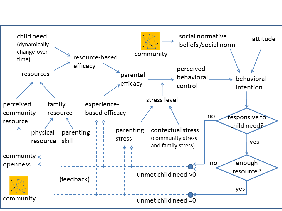
Figure 1. Model of A Single Agent - 3.3
- The
model uses a child's unmet need as a measure of child maltreatment.
Unmet need is the difference between the child need and the child care
provided. Throughout this paper we will use the terms "child
maltreatment" and "unmet need" interchangeably for readability. We do
not differentiate between different forms of child maltreatment, but
our resource-based approach is most applicable to studying child
neglect as oppose to other types of child maltreatment such as
emotional abuse and sexual abuse. Note that although each agent is
modeled in detail through the cognitive modeling, the main focus of the
developed model is on studying the macro-level behavior, i.e., how the
interaction of these agents results in communities with different
levels of CM. Also note that the purpose of this paper is to present a
model that explores the possible dynamics of CM without an attempt to
have fidelity to real world observations (model calibration and
validation from real world data will be an effort of future work).
Because of this, some parameter values used in the model are
empirically determined based on what we think are reasonable within the
context of CM. Due to the same reason, we simplify the quantification
of all the elements of our model by representing them on an arbitrary
scale of 0–100 (except for parenting stress and contextual stress). The
units of the scale are purposely not specified in order to simply
represent relative values of the variables under study. Below we
describe the model elements in detail.
Child Need and Family Resource
- 3.4
- The child need represents
the amount of care a child or children require in a family. To model
that different families have different child need, we use a child need base, denoted as Nbase,
to represent the average of an agent's child need. For example, a
family with a child with a developmental disability will have a higher
child need base, than another family without a disabled child. Also,
families with more children will have higher overall child need, which
is represented with a higher child need base. Although children have an
average level of need, their actual day to day needs fluctuate. To
model this, an agent's actual child need (denoted as Nchild) in a time step is dynamically generated by oscillating within a range (denoted as Nrange)
based on its child need base. In the current model, the child need is
generated following a uniform distribution within the range, as denoted
below:
Nchild ∼ [Nbase − Nrange/2, Nbase + Nrange/2] (1) - 3.5
- The family resource
represents the resources of a family for taking care of children. A
family's resources are affected by a family's social and economic
situation. In general, a family is considered to have more resource if
there are two parents living in the house to help with the child care
(compared to one parent, such as a single mom); a family has more
resource if the family's economic condition is supportive for providing
care. In our model, we refer to the resources related to social and
economic situations as physical resource, denoted as Rphysical.
Besides the physical resources, the skills of parents (i.e., parenting
skill) are also considered as part of the internal resources of a
family (Hillson & Kuiper 1994).
Parenting skill represents how efficiently the physical resources are
used for child care. To model this, we define parenting skill as a
coefficient, denoted as kparentingskill, and model a family's resource Rfamily as the product of the family's physical resource and its parenting skill coefficient.
Rfamily = Rphysical × kparentingskill (2) - 3.6
- Both
the child need and family resource are individualized properties of an
agent. Different agents of the same community have different child need
and family resource, reflecting that families are different. In the
current model, Nbase, Rphysical, and kparentingskill
are initialized in the beginning of the simulation and do not change
over time (unless a specific CM prevention program, e.g., parent
training to improve parenting skill, is implemented). To set up an
"artificial community" to run simulations, agents can be created with
randomly generated Nbase, Rphysical, and kparentingskill
based on overall characteristics of the community, e.g., average number
of children per household, average number of parents per household, and
average parenting skill.
Social Network and Community Openness
- 3.7
- The ABM views a community not only as a living environment, but also a potential resource for obtaining support in providing child care. A community's social structure is defined by the social network. Each agent is connected to some other "neighbor agents" through its social network. In the current implementation, the social network among agents is a scale-free network. It is generated using the preferential attachment algorithm of Barabasi and Albert (1999) in which the probability a new node links to existing nodes is increasing in the number of links the existing node already has, creating a positive feedback loop through which popular nodes become even more popular. The community social structure can be modeled in other types of networks, e.g, a small world network, that may better reflect the network structure among families in the CM context (this will be explored in future work). The social network structure is initialized in the beginning of the simulation and does not change over time. However, a CM prevention program, e.g., the "build social connections" program described later, can change the social network over time.
- 3.8
- Some families are more receptive to interacting with their neighbors than other families. The degree to which families are willing to interact with their neighbors is represented in our model by the community openness variable, denoted as γ . The community openness influences the likelihood of an agent to ask for support from its neighbors in order to meet its child need. In general, the higher an agent's community openness is, the more likely the agent will ask for support from neighbors if needed. In our model, this likelihood is specified by a community involvement probability (denoted as α), which is calculated based on the agent's community openness ( α = 0.01 * γ). Note that it is possible for an agent to have no neighbors (socially isolated). In this case, the agent is not able to ask for support.
- 3.9
- As a
simulation proceeds, an agent's community openness is dynamically
updated based on the agent's experience in the community (a feedback
mechanism). An agent's community openness is updated at a time step
only when it asks for community support. Specifically, if the agent
asks for support and successfully gets enough support to meet its child
need, it increases γ; otherwise if the agent asks for support but
receives no support or does not get enough support to meet its child
need, it decreases γ. The dynamically changing community openness will
then influence the agent's likelihood of community involvement in the
future. Equation (3) shows how the community openness γ is updated. The
number 0.3 and 0.15 represent the amount of change – they are
relatively small because the change happens in every step of the
simulation. Note that the decrease of γ in the second case is less than
that in the third case because in the second case the agent receives
support from neighbors even though it still has unmet child need.
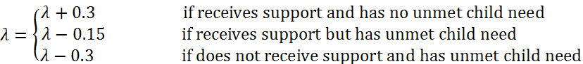
(3) Parental Efficacy
- 3.10
- An agent's parental efficacy (denoted as Eparental),
defines the agent's belief about its capability of taking care of its
children (i.e., meeting child need). In our work, an agent's parental
efficacy is formed from two sources: the resource-based efficacy (denoted as Eresource) and the experience-based efficacy (denoted as Eexperience).
The resource-based efficacy captures the portion of efficacy induced
from the available resources compared to the child need. In our model,
the total resource of an agent perceived to be available for child care
includes the family resource Rfamily (defined in Equation (2)) and the resources perceived as being available in the community. The latter is referred to as the perceived community resource (denoted as Rperceived). To calculate Rperceived,
an agent estimates the spare resources of its neighbors (if any) by
evaluating how many resources it expects them to have after handling
their own children. The expected surplus resources of a neighbor are
determined from the difference between that neighbor's family resource
(denoted as
 ) and child need base (denoted as
  ).
The neighbor resource is the sum of surplus resources from all
neighbors. The perceived community resource of an agent depends on not
only the neighbor resource, but also the willingness of the agent to
utilize the neighbor resource. This willingness is captured by the
agent's community involvement probability α, which depends on the
community openness γ of the agent. If an agent's community openness is
low, its Rperceived will be low even though there may be a high level of available resources from neighbors. Overall, an agent's Rperceived is computed as the product of the agent's community involvement probability and the neighbor resource.
).
The neighbor resource is the sum of surplus resources from all
neighbors. The perceived community resource of an agent depends on not
only the neighbor resource, but also the willingness of the agent to
utilize the neighbor resource. This willingness is captured by the
agent's community involvement probability α, which depends on the
community openness γ of the agent. If an agent's community openness is
low, its Rperceived will be low even though there may be a high level of available resources from neighbors. Overall, an agent's Rperceived is computed as the product of the agent's community involvement probability and the neighbor resource.

(4) - 3.11
- The total resource Rtotal of an agent is the sum of the agent's family resource Rfamily and the perceived community resource Rperceived. The resource-based efficacy Eresource
of a time step depends on the difference between the total resource and
child need at that time step – the larger the difference, the higher
the resource-based efficacy. This relationship is described by the
equations below, which shows how the resource-based efficacy is
calculated from the difference between resource and child need. In our
model, we scale the disparity between total resource and child need by
1.25 and add 50 to bring its numerical value in line with the other
parameters. When the total resource equals to the child need, the
resource-based efficacy is 50, which is half of the full resource-based
efficacy.
Rtotal = Rfamily + Rpercieved (5) Eresource = 50 + (Rtotal − Nchild) × 1.25 (6) - 3.12
- Different
from the resource-based efficacy, the experience-based efficacy
captures the portion of efficacy induced from the agent's past
experience of child care. The experience-based efficacy changes over
time and is dynamically updated in each time step based on the agent's
experience of meeting the child need. In general, if the agent
successfully meets the child need, its experience-based efficacy
increases; otherwise, its experience-based efficacy decreases. The
following equations show how the experience-based efficacy is increased
or decreased in a time step based on whether the child need is met or
not in that time step. In equation (8), the amount of unmet child need
of that time step is denoted as Nunmet. Nunmet=0 means there is no unmet child need and Nunmet>0 means there exists unmet child need. The coefficient kceiling
is used to model the ceiling effect when increasing experience-based
efficacy: as the experience-based efficacy becomes larger, the increase
rate of the experience-based efficacy becomes slower.
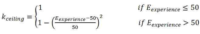
(7) 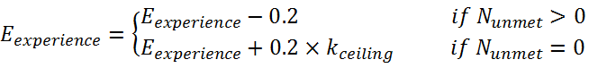
(8) - 3.13
- The
parental efficacy is the weighted sum of the resource-based efficacy
and experience-based efficacy, as shown in Equation (9). We assign a
slightly larger weight for the experience-based efficacy because we
consider parent-child interactions as routine events. Under routine
circumstances, an individual may well utilize the previous performance
level (obtained from experience) as the primary determinant of
self-efficacy (Gist & Mitchell 1992).
Eparental = 0.6 × Eexperience + 0.4 × Eresource (9) Stress Level
- 3.14
- An agent's stress level (denoted as Stotal) comes from two different sources: contextual stress, (denoted as Scontextual) and parenting stress (denoted as Sparenting). Multiple contextual sources of stress are discussed in Belsky (1984). In our work, contextual stress is composed of community stress (denoted as Scommunity) and family stress (denoted as Sfamily) as shown in equation (10). The community stress represents stressors such as crime in the neighborhood and the family stress represents
stressors such as divorce. During a simulation, all agents in the same
community share the same community stress, but different agents have
different family stress levels. The values of the community stress and
family stress of an agent are initialized in the beginning of the
simulation and are assumed to be unchanged throughout the simulation.
Scontextual = Scommunity + Sfamily (10) - 3.15
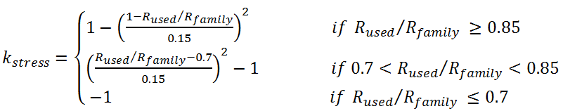
- The parenting stress Sparenting is influenced by the disparity between the demands of parenting and the resources to fulfill those demands (Abidin 1995).
The parenting stress is dynamic in nature. It is updated in each time
step based on the amount of resource that is used (denoted as Rused, defined in section 3.6) in that time step compared to the overall family resource of the agent. More specifically, when Rused is much less than the family resource, the parenting stress decreases over time; otherwise when Rused
is close to the full capacity of family resource, the parenting stress
increases over time. Equation (12) shows how the parenting stress is
updated based on the ratio of used resource and family resource. In the
equation, 0.85 is the threshold ratio (denoted as Sthreshold).
We use this threshold ratio to model how a parent changes his/her
parenting stress: when more than 85% of the family resource is used,
parenting stress increases; otherwise parenting stress decreases. In
the equation, the coefficient kstress defines the
increase or decrease rate based on the distance to the threshold ratio.
For example, a family that only barely crosses the 0.85 threshold for
used resource will increase its parenting stress much less than a
family that uses all of its family resources.
(11) 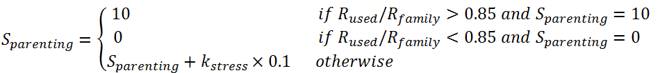
(12) - 3.16
- In
our model, the parenting stress is in the range of 0 to 10. The
contextual stress is in the range of 0 to 20 to account for the two
sources of contextual stress: Scommunity and Sfamily, each of which is in the range of 0 to 10. We chose to use the 0 to 10 scale for Scommunity, Sfamily, and Sparenting
to make tuning the model more intuitive. An agent's total stress level
is the sum of its contextual stress and parenting stress as shown in
equation (13), where the coefficient 10/3 converts the total stress
level to the 100 scale to be consistent with the scale we use for our
other variables.
Stotal = (Scontextual + Sparenting) × 10/3 (13) Behavioral Intention
- 3.17
- The Theory of Planned Behavior (TPB), proposed by Ajzen (1991)
is used to calculate an agent's behavioral intention of taking care of
its children. According to TPB, the behavioral intention is determined
by the attitude towards child care, the social norms surrounding child
care in the community, and the perceived behavioral control (denoted as
PBC). The perceived behavioral control (PBC) represents how much
control parents think they have over their child's wellbeing. In our
model, PBC is the result of parental efficacy Eparental modulated by the stress level Stotal. This is shown by equation (15), where kefficacy
is the stress-based coefficient that modulates the parental efficacy
into the PBC. In general, the higher the stress level, the smaller the
stress-based coefficient. Equation (14) shows how kefficacy is calculated based on the stress level.
kefficacy = 1 − (Stotal/100)2 (14) PBC = kefficacy × Eparental (15) - 3.18
- Based
on TPB, an agent's behavioral intention is calculated from the
perceived behavioral control (PBC), attitude (denoted as AT), and
social norm (denoted as SN), multiplying by their corresponding
weights. The attitude indicates a family's general tendency or
orientation towards parenting behavior. The social norm reflects the
social context of the agent. In our model, social norm is set as the
average attitude of the entire community. The weights wattitude, wsocialnorm, wPBC
define the relative percentages of contribution of the three elements:
attitude, social norm, and PBC in computing the behavioral intention.
In our model, these weights are determined based on the level of PBC:
when an agent has high level of PBC (higher than 70 in our model), the
attitude, social norm, and PBC have about the same weight (0.35, 0.35,
and 0.3, respectively); as the level of PBC drops, the weight for the
PBC becomes larger. This approach, to some extent, incorporates the
idea of "hot" cognition (Abelson 1963),
which is a motivated reasoning phenomenon in which a person's responses
(often emotional) to stimuli are heightened. Equation (16)–(18) show
how the three weights are calculated.
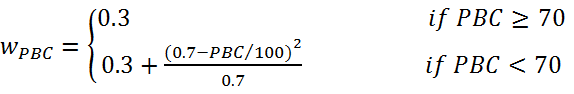
(16) wattitude = (1 − wPBC)/2 (17) wsocialnorm = (1 − wPBC)/2 (18) - 3.19
- Based
on its attitude, social norm, and PBC, an agent's behavioral intention
(denoted as I, in the range of 0 to 100) is the weighted sum of them as
shown in Equation (19). This intention determines the agent's
probability (denoted as prob, see Equation (11)) of choosing the "responsive to child need"
behavior. The higher the intention level, the more likely the agent
will be engaged in the parenting behavior for meeting the child need.
I = wattitude × AT + wsocialnorm × SN + wPBC × PBC (19) prob = I/100 (20) - 3.20
- If
the "responsive to child need" behavior is chosen, the next step is to
check if the agent actually has the resources (family resource plus
community resource) to meet its child need. In our model, parents who
are responsive to their children's needs will make every attempt to
take care of them. Parents who are not responsive will only provide
care according to the intention level (which may or may not meet the
child need). The next two sub-sections describe how an agent does when
it is responsive to its child's needs and how it does when it is not.
Responsive to Child Need
- 3.21
- Parents who are responsive to their children's needs will make every attempt to take care of them, including using their own family resource and seeking support from neighbors in their social network. In order not to significantly increase the parenting stress (see section 3.5), we assume an agent only wants to use its own family resource up to a "comfortable level" if it can also get neighbor or community support. Only when the "comfortable level" of care from its own family resource plus the neighbor support (if any) together cannot meet the child need, the agent uses its family resource beyond the comfortable level. Note that if child need is very high, an agent may have to use all its family resource but still cannot meet the child need.
- 3.22
- Specifically, when an agent chooses the "responsive to child need" behavior, it goes through the following three steps to compute the amount of child care for meeting the child need.
- 3.23
- Step 1: calculate the "comfortable level" of care (denoted as CAREcomfortable). If CAREcomfortable is greater than child need Nchild, this means the "comfortable level" of care is enough to meet the child need. In this case, the child need is met (Nunmet=0), i.e., there is no unmet child need for this step. The agent skips the next two steps. Equation (21) shows how CAREcomfortable is calculated. In the equation, Sthreshold is the threshold ratio above which the parenting stress increases (discussed in Section 3.5). Since Sthreshold is 0.85 in our model, CAREcomfortable is equal to 92.5% of Rfamily.
This means that parenting stress will increase even when a comfortable
level of care is provided, which is in keeping with our observation
that child care is stressful.
CAREcomfortable = Rfamily * (0.5 + Sthreshold/2) (20) - 3.24
- Step 2: If an agent's comfortable level of care is less than child need (CAREcomfortable < Nchild), the next step is to check if the agent can get support from neighbors through its social network. An agent does not get any neighbor support if it either has no neighbor or it is not willing to ask for support (an agent's willingness of asking for support is determined by its community involvement probability α defined in section 3.3). If an agent does ask for support, it asks for help from its neighbors in a random order until it is either able to completely meet its child need, or it runs out of neighbors to ask. A neighbor that is asked for support decides whether to offer resource by looking at how much resource it has already used. Specifically, it checks the used family resource (denoted as Rused) and compares it with its "comfortable level" of care CAREcomfortable defined in equation (21). If the used resource is less than CAREcomfortable, it provides support up to CAREcomfortable; otherwise it does not provide support. If an agent gets enough support from neighbors to meet its child need, the child need is met (Nunmet=0) and the agent skips the next step.
- 3.25
- Step 3: If after asking neighbors for support an agent still has unmet need, then it will use up its remaining resource on child care. If the remaining resource is able to meet the child need, the child need is met (Nunmet=0). Otherwise, there exist unmet child and Nunmet is equal to the difference between the child need and the total care, which is the amount of care from both the agent's own family resource and from neighbor support.
- 3.26
- After all these steps, an agent's overall used family resource Rused is the resource used in taking care of its own children plus the resource used to support neighbors. The Rused influences how the agent's parenting stress is updated (see section 3.5).
Unresponsive to Child Need
- 3.27
- Even when
families are neglectful they still provide some child care. In our
model, if the "responsive to child need" behavior is not chosen, the
agent is not committed to be responsive to child need. In this case,
the agent simply provides what we call intention-based care (denoted as CAREintention) and will not seek neighbor support. The CAREintention
is proportional to the child care behavioral intention as shown in
equation (22). With the intention-based care, the unmet child need Nunmet is equal to the difference between the child need and CAREintention; the Rused is equal to CAREintention.
We note that although intention-based care is given when a family is
not responsive to child need, it is still possible (although unlikely)
that it is enough to meet the agent's child need (in that case, Nunmet=0).
CAREintention = Rfamily * (I / 100) (22) CM Prevention Modeling
- 3.28
- The ABM can also be used to support simulating the impact of different CM prevention or intervention programs. To model a CM prevention/intervention program, the basic idea is to identify the pathways for the program to exert influence in the system. Different CM preventions/intervention programs influence families and their connections through different pathways. For example, community resource center influences the system by providing resources to families in the community. To model CM prevention, special types of agents may be developed to carry out the pathways of influence or to represent entities involved in the prevention/intervention programs (e.g., service providers, social workers). For example, to model a community resource center, a "community resource center" agent can be developed and added to the system. This agent is connected to all family agents in the community, reflecting that it is accessible to all families in the community.
- 3.29
- As
illustrative examples of CM prevention modeling, we modeled three basic
CM prevention strategies in our work and evaluated their impacts
through experiments (experiment results are shown in section 4.4). The three strategies are: community resource center, neighborhood development to reduce community stress, and build social connections. Each of these strategies targets a particular influential model component. The three strategies are described below.
- Community resource center. This preventive strategy provides resources to families in the community in each time step. The community resource center is specified by a capacity that represents the maximal number of families it can support in each time step. To model this strategy, a "community resource center" agent is created to provide resource to family agents who request support until its capacity is reached. We note that for simplicity we assume when the community resource center helps a family, its resource is committed to the family for only one time step (instead of a period of time). The resource is available to all family agents in the next time step. Also note that when a community resource center has limited resources, simulations can be carried out to study how different ways of prioritizing families for receiving the support may impact the overall outcome of CM (Keller & Hu 2013).
- Neighborhood development to reduce community stress. This preventive strategy reduces the community stress (which is part of the contextual stress of families) through neighborhood development such as reducing crime rate. This strategy takes place over time. It is specified by a target community stress reduction rate (denoted as Rate) and a time for the strategy to reach its full target result, also called time to full result (denoted as Time, in number of days). For example, Rate = 70% and Time = 365 mean the original community stress level will be reduced by 70% in one year. To model this strategy, in each time step (up to time step T) the community stress is reduced by an amount that is equal to the original stress level times the daily reduction rate (which is Rate/Time).
- Build social connections. This preventive strategy adds social connections between families. Similar to the above strategy, this strategy takes place over time. It is specified by a target improvement rate (denoted as Rate) and a time to full result (denoted as Time, in number of days). For example, Rate = 30% and Time = 365 mean the total number of social connections of the community will be increased by 30% in one based on the initial number of social connections in the social network. To model this strategy, in each time step (up to time step T) a number of new social connections will be added. The number of new connections to be added in each step is equal to the total number of new connections to be added divided by T.
Simulation Procedure and Dynamics of the Model
- 3.30
- Simulation of the ABM runs in a step-wise fashion, where each time step represents one day. In every time step, for each agent a child need is dynamically generated based on the agent's child need base and oscillating range (section 3.2). The parental efficacy is then computed from the experience-based efficacy and resource-based efficacy, which is based on the difference between family resource and child need in that time step (section 3.4). The stress level is also computed from the contextual stress and the parenting stress in that time step (section 3.5). Then the perceived behavioral control and the behavioral intention are calculated to determine the probability of choosing "responsive to child need" behavior (section 3.6). After that the corresponding steps (including seeking for support from neighbors if needed) for the "responsive to child need" or "unresponsive to child need" behaviors are carried out to determine if there is unmet child need (section 3.6.1 and section 3.6.2). Finally, due to the feedback loops, the parenting stress, experience-based efficacy, and community openness are updated and the simulation proceeds to the next time step.
- 3.31
- There are three direct feedback loops in the current model. The first one is related to parenting stress: if in a time step the ratio of used resource compared to the overall family resource (Rused/Rfamily) is higher than a threshold, the parenting stress increases; otherwise the parenting stress decreases (section 3.5). The second one is related to experience-based efficacy: if in a time step there is no unmet child need (Nunmet=0), that is, no child maltreatment, the experience-based efficacy increases; otherwise it decreases (section 3.4). The third one is related to community openness. If in a time step an agent receives support from neighbors and has no unmet child need, its community openness increases. Otherwise the community openness decreases (section 3.3). These feedback loops at multiple levels of the social ecology together with the fluctuations of child need in each time step result in dynamic and complex behaviors of the ABM.
Experiment Results
-
Simulation Setup
- 4.1
- We carry out a series of experiments to evaluate and to demonstrate the utility of the ABM. Before a simulation starts, an "artificial community" with multiple family agents needs to be created. Different agents can have different properties, reflecting that families are different in the real world. Below we describe how we assign agents' properties when an agent is created. In all our experiments (unless otherwise noted), an agent's child need base Nbase is drawn from a uniform distribution over the range [75, 85]. This is denoted as Nbase ∼ [75, 85] (the same notation is used for other properties whose values are drawn from uniform distributions). Its child need oscillating range Nrange = 10; family physical resource Rphysical ∼ [76, 92], parenting skill coefficient kparentingskill ∼ [0.5, 0.7], community openness γ ∼ [50, 70], initial experience-based efficacy Eexperience = 60 (note: Eexperience changes over time during the simulation), family stress Sfamily = 5, initial parenting stress Sparenting = 0 (note: Sparenting changes over time during the simulation), attitude AT =80, community stress Scommunity = 4 (for low risk community), 8 (for high risk community). All other model parameters are the same as those described in the previous model section. Note that in this paper we choose to use the uniform distribution to draw values from a range. A different choice would be a normal distribution, which will be considered in future work. There are 100 families (agents) in the community and each community is simulated for 1000 time steps. Each experimental result is the average of 100 simulations. The experiments were carried out using Repast version 3 (http://repast.sourceforge.net), which is a Java agent-based modeling toolkit.
- 4.2
- For the purposes of our experiments, we consider two types of communities, named as a high stress community and a low stress community, where stress refers to the community stress level. In the high stress community, community stress Scommunity is set to 8, whereas in the low stress community it is set to 4. All other parameters are the same between the two communities, so as to study the impact of community stress on child maltreatment. To measure child maltreatment outcome, we define a family that has unmet child need (Nunmet>0) in more than 350 steps of the 1000 time steps as being a high risk family (HRF). We use the phrase "high risk" to describe the families because they do not meet their child needs for significant number of time steps during the simulation and thus have a high risk of child maltreatment. In presenting the aggregated results of a community or subgroup, we use the fraction of high risk families, defined as the ratio of the HRF number over the total family number, in the entire community or subgroup as a measure of child maltreatment risk of the community or subgroup. For readability we will use the phrases "fraction of high risk families (HRF fraction)" and "child maltreatment (CM) risk" interchangeably.
- 4.3
- We carry out experiments to evaluate and demonstrate different aspects of the model. The first experiment (section 4.2)
aims to study the parameter sensitivity for four important model
parameters: parenting skill, initial experience based efficacy, initial
community openness, and community stress. The second experiment
(section 4.3) examines family
heterogeneity in a community and shows how the heterogeneity influences
child maltreatment outcomes. The third experiment (section 4.4) simulates the impacts of different CM prevention strategies and compares their results.
Parameter Sensitivity
- 4.4
- Parenting skill,
initial experience based efficacy, initial community openness, and
community stress are four important variables. To study these variables
we ran experiments over their entire range of values in increments
equal to 1/100th of their ranges. When we vary the value of one
parameter, we make all agents share the same value for that parameter
and fix the values for all other parameters using their default values
described in section 4.1. For example,
when simulating the impact of parenting skill with value 0, the
parenting skill coefficient of all agents is set to 0. When studying
parenting skill, initial experience based efficacy and initial
community openness, the community stress is set to be 4 (a low stress
community). For each possible value we ran 100 trials and averaged the
HRF fraction in the communities. The plots for these four variables are
shown in figure 2 below. Recall that parenting
skill coefficient is in [0, 1], initial experience based efficacy is in
[0, 100], initial community openness is in [0, 100], however, community
stress is in [0, 10], which is why we use the "% of maximum range" as
the x-axis scale.
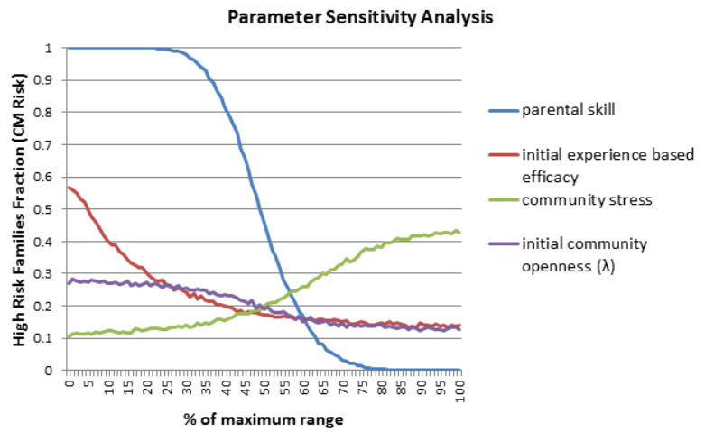
Figure 2. Parameter sensitivity for parental skill, initial experience-based efficacy, initial community openness (λ), and community stress - 4.5
- The first thing to observe is that the general patterns for all four parameters are as expected. As parenting skill, initial experience-based efficacy, or initial community openness increases child maltreatment risk decreases. As community stress increases, so does child maltreatment. Parenting skill, initial community openness, and community stress all have non-linear "s curves." Parenting skill has the largest impact on child maltreatment risk because it has the largest change in HRF fraction when going from 0% to 100% of its maximum value. The significance of parenting skill is understandable because the increase of parenting skill results in higher family resource (see Equation (2)). When parenting skill is low, the HRF fraction maintains at a high level because families are categorized as high risk families as long as they have unmet child need in more than 350 time steps. The increase of community stress impacts all families by increasing families' stress level, and thus decreasing families' perceived behavioral control through the modulation mechanism described in Equation (14). The results in Figure 2 show that when parenting skill is extremely low (or community stress is extremely high), a small increase of parenting skill (or decrease of community stress) does not have a significant impact.
- 4.6
- The impact of
initial experience based efficacy follows a different pattern. Recall,
that experience based efficacy reflects a family's assessment of their
ability to take care of their children based upon prior child care
experiences. Unlike parenting skill and community stress, which
maintain invariant during the simulation, experience based efficacy is
given an initial value (initial experience based efficacy) when a
simulation starts and is then dynamically updated as the simulation
progresses. Figure 2 shows that when families have
a low experience based efficacy to start with, they has a high chance
to have child maltreatment. This mirrors the literature on efficacy by
showing the significant impact that an agent's level of "confidence"
can have on their ability to complete a task, which is in this case
child care. A reinforcing loop means that the effect of a particularly
low or high initial experience based efficacy persists throughout the
simulation. The results also show that when the initial experience
based efficacy is extremely low, even a small increase of it (e.g.,
through interventions) can make a real difference. Similar to the
experience-based efficacy, an agent's community openness is also
dynamically updated over time depending on if the agent receives
support from neighbors and if it has unmet child need (Equation (3)).
Nevertheless, the impact of the initial community openness is
relatively small compared to the three other parameters. Even when
agents' initial community openness is low in the beginning, the overall
HRF fraction is still less than 30%. This is because the community
under study is a low stress community, and agents are able to either
satisfy their own child need or increase their community openness over
time.
Family Heterogeneity in a Community
- 4.7
- The advantage of agent-based modeling is that we can look at intra-community heterogeneity. In this experiment, we examine family heterogeneity in a community and shows how the heterogeneity influences child maltreatment outcomes. Families can be classified according to their number of social resources (the number of neighbors they have), and their ratio of family resources to child need. These two categorization schemes are appropriate, because families can help their children on their own, or they can get help from neighbors. Two families can have the same amount of family resources, but different child need, so only the ratio of family resource to child need fully captures how easily a family can meet its child need before seeking outside assistance from neighbors or other sources. We define the ratio as Rfamily/Nbase. Whenever the ratio is above 1 it can be thought of as the % extra resources, so for example, if the ratio equals 1.1, then the % extra resource is 10%. The 0% extra resource group means the family resources of these families are less than their child need base.
- 4.8
- We chose three groupings for the number of neighbors and four groupings for the % extra resources. Figure 3
shows the groupings and their proportions (number of families in each
group) for a typical community simulated in our experiment. Note that
there are total 100 families in the community.
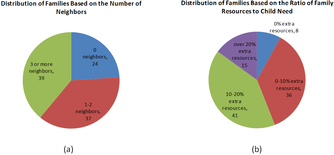
Figure 3. Heterogeneity within a Community. (a) Grouping by number of neighbors. (b) Grouping by % extra resources. - 4.9
- If
these groupings are significant then we would expect to see different
CM rates across them. More specifically, the more neighbors and the
more extra resources a family has the lower its rate of CM should be.
Additionally, a high stress community with a community stress of 8
should have more CM risk across all categories of families than a low
stress community with a community stress of 4. These expectations are
confirmed in figure 4 below. Figure 4(a) shows the proportion of high risk families in subgroups determined by the number of neighbors a family has. Figure 4(b) shows the proportion of high risk families in subgroups defined by the % extra resources. In figure 4,
the blue bar represents the results from the low stress community, and
the red bar represents the results from the high stress community. The
last category, "all families", represents the proportion of high risk
families in the entire community.
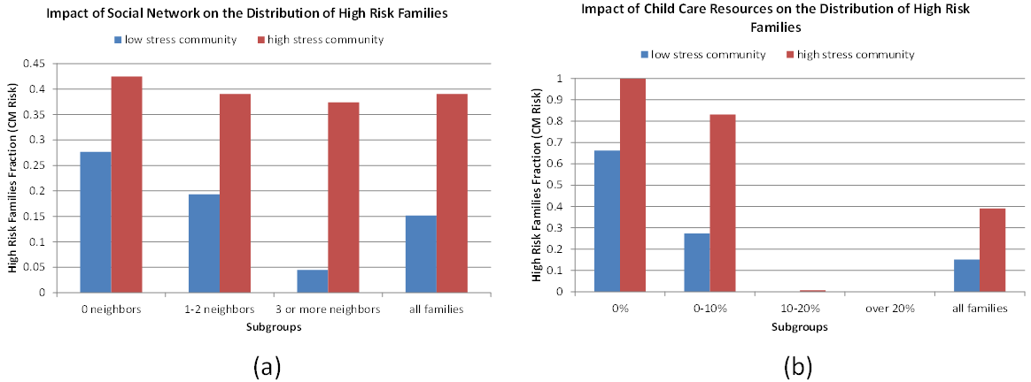
Figure 4. Impact of Family Heterogeneity on CM outcome: (a) number of neighbors (b) % extra resources - 4.10
- In all cases the high stress community had the same or higher rates of CM than the low stress community. This is expected because the community stress is shared by all families in the community and impacts all subgroups. For a particular community type (low stress community or high stress community), the different subgroups have different CM risk outcomes. As expected, more neighbors lead to lower HRF fraction, and more % extra resources lead to lower HRF fraction. When % extra recourse is 10-20% or more, the HRF fraction is zero (or close to zero) for both communities.
- 4.11
- The amount of difference of the results among the subgroups, however, is different for the two communities. In the low stress community, the difference among the subgroups is more significant. For example, for the subgroups of "1-2 neighbors" and "3 or more neighbors", in the low stress community the HRF fraction changes from 19% to 4% (a 15% change). But in the high stress community, the change is from 38% to 36% (only a 2% change). The same can be seen for the subgroups based on % extra resources. When the % extra resource changes from 0% to 0–10%, for the low stress community the HRF fraction change from 65% to 26% (a 39% change). But for the high stress community, it is changed from 100% to 82% (only a 18% change). This difference between the low stress community and high stress community is because in the high stress community families have high stress levels. Based on the model, families with high stress levels tend not to fully exploit their family resources and/or social connections (due to low behavioral intention). Thus even families may have extra resources or social connections, they do not fully exploit these resources and thus the difference among the subgroups is less significant. When the community stress is reduced as in the low stress community, families with more social connections or more family resources can significantly reduce the HRF fraction because they begin to exploit these resources. Families with less resource/social connections "benefit" in a limited way because they have limited resources to exploit.
- 4.12
- This
experiment shows that sub-dividing the community based on the number of
neighbors and the % extra resources results in qualitatively different
distributions of CM among the subgroups. The results show that
heterogeneity in a community matters. They also indicate that when a CM
prevention or intervention program (e.g., reducing community stress
from high to low) is implemented, it can have different levels of
impacts on different subgroups in the community.
CM Prevention Simulation
- 4.13
- We model three
CM prevention strategies and simulate their impact on CM outcome. We
carry out the simulations using the high stress community (community
stress =8). The three prevention strategies are community resource
center, neighborhood development to reduce community stress, and build
social network. They are described in section 3.7.
For the community resource center strategy, we vary its capacity from 0
to 20 (0 means no prevention). For the reduce community stress and
build social network strategies, we use 1 year (365 time steps) as the time to full result
and vary the target rate from 0 to 100% (0 means no prevention). In all
cases, we measure the HRF fraction of the whole community. Figure 5(a) shows the results for the reduce community stress and build social network preventions, and Figure 5(b) shows the community resource center prevention. In Figure 5(a)
the x-axis represents the target reduction rate or improvement rate of
the preventions. When the target rate equals 1, the community stress is
reduced to 0 (if the reduce community stress prevention is being
studied) and the total number of social connections of the community
doubles (if the build social network prevention is being studied).
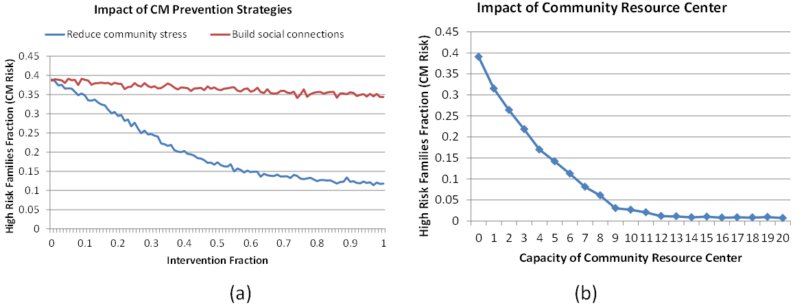
Figure 5. Impact of CM preventions: (a) reduce community stress and build social network; (b) community resource center - 4.14
- Figure 5(a) shows that as the prevention target rate increases, the HRF fraction decreases for both the reduce community stress and build social network preventions. The impact of the community stress reduction is non-linear; there is a point of diminishing returns around the 50% community stress decrease point. It is important from a policy perspective to be aware and then try to identify the point of diminishing returns for the reduce community stress prevention. The result from the build social network prevention shows a modest decrease in the HRF fraction in the community. This means that by increasing the interconnection of families CM risk can be reduced even if the total resources in the community are not increased. For this community, it is unsurprising that decreasing community stress has a greater impact than building the social network, because this is a high stress community. As discussed earlier, when the community stress is high, families tend not to fully exploit the social connections, thus building social connections has a limited impact in this case. However, as shown in Figure 4(a), in a low stress community, when social connections increase from "1-2 neighbors" to "3 or more neighbors", the HRF fraction decreases from 19% to 4%. This means for such a community the build social network prevention can have a much greater impact.
- 4.15
- The results of the community resource center are shown in figure 5(b). The x-axis represents the capacity, i.e., the number of families that can be helped in each simulation step. As can be seen, when the capacity is 0, which means no prevention is applied, about 38% out of 100 families are high risk families. Figure 5(b) shows that there is no need to have a capacity of 38 to reduce the HRF rate to 0. In fact, when the capacity reaches 10 the number of high risk families in the community is almost zero. This is due to the following reasons caused by two feedback loops existing in the system. On one hand, at the individual family level, when a family's unmet child need drops to zero as a result of getting help from a community resource center its experience-based efficacy increases, which makes it more likely to take care of its children using its own family resource in the future, which will in turn increase its experience-based efficacy further. On the other hand, at the community level, when families benefit from the community resource center, they increase their community openness, which in turn makes it more likely for families to support each other through social network and thus reduces the need of support from the community resource center.
Conclusions
- 5.1
- This paper presents an agent-based model for simulating the dynamics of child maltreatment and child maltreatment prevention, and shows experiments results covering different aspects of the model. Development of this model was a result of an iterative modeling process, with inputs from domain experts in CM research. To our knowledge this is one of the first agent-based models employing systems science methodologies to study CM and CM prevention. Future work includes model validation from empirical data and applying the model to supporting CM prevention research. The purpose of this work is to present a model that explores the possible dynamics of CM and helps studying CM prevention/intervention. Computer models of child maltreatment do not replace field studies, but they can provide useful information for advancing child maltreatment prevention. We hope this work can inspire further modeling work in this field.
Acknowledgements
- This work was supported in part by a CDC-GSU seed grant. We thank Richard Puddy, PhD, and Charlyn H. Browne, PhD, for their collaboration in developing the model.
References
-
ABELSON, R. P. (1963). Computer simulation of "hot cognition", Computer simulation of personality, 277–302
ABIDIN, R. R. (1995). Parenting Stress Index: Professional Manual (3rd ed.). Odessa, FL: Psychological Assessment Resources, Inc.
AJZEN, I. (1985). From intentions to actions: A theory of planned behavior. In J. Kuhl & J. Beckman (Eds.), Action-control: From cognition to behavior (pp. 11–39). Heidelberg: Springer.
AJZEN, I. (1991). The theory of planned behavior. Organizational Behavior and Human Decision Processes, 50, 179–211. [doi:10.1016/0749-5978(91)90020-T]
BANDURA, A. (1977). Self-efficacy: Toward a unifying theory of behavioral change. Psychological Review, 84, 191.215. [doi:10.1037/0033-295X.84.2.191]
BANDURA, A. (1982). Self-efficacy mechanism in human agency. American Psychologist, 37, 122–147. [doi:10.1037/0003-066X.37.2.122]
BANDURA, A. (1994). Self-efficacy. In V. S. Ramachaudran (Ed.), Encyclopedia of human behavior (Vol. 4, pp. 71–81). New York: Academic Press. (Reprinted in H. Friedman [Ed.], Encyclopedia of mental health. San Diego: Academic Press, 1998).
BARABASI, A. L. & R. Albert. (1999). Emergence of scaling in random networks. Science, 286(5439), 509–512.
BELSKY, J. (1980). Child maltreatment: An ecological model. American Psychologist, 35(4), 320–335. [doi:10.1037/0003-066X.35.4.320]
BELSKY, J. (1984). The determinants of parenting: A process model. Child Development, 55, 83–96. [doi:10.2307/1129836]
DAHLBERG, L. L. & Krug, E. G. (2002). Violence a global public health problem. In: E. Krug, L. L. Dahlberg, J. A. Mercy, A. B. Zwi, & R. Lozano, eds. World Report on Violence and Health. Geneva, Switzerland: World Health Organization, 1–56.
FREISTHLER, B., Merritt, D. & LaScala, E. (2006). Understanding the ecology of child maltreatment: A review of the literature and directions for future research. Child Maltreatment, 11, 263–280. [doi:10.1177/1077559506289524]
GIST, M. E. & Mitchell, T. R. (April 1992), Self-Efficacy: A Theoretical Analysis of Its Determinants and Malleability, The Academy of Management Review, 17(2), 183–211.
HAMMOND, R. A. (2009). Complex systems modeling for obesity research. Preventing Chronic Disease: Public Health Research, Practice, and Policy, 2009; 6(3).
HILLSON, J. M. C. & Kuiper, N. A. (1994). A stress and coping model of child maltreatment. Clinical Psychology Review, 14, 261–285 [doi:10.1016/0272-7358(94)90025-6]
HU, X. & Puddy, R. (2010). An Agent-based Model for Studying Child Maltreatment and Child Maltreatment Prevention, Proc. 2010 International Conference on Social Computing, Behavioral Modeling, & Prediction (SBP10), pp. 189–198, 2010
HU, X. & Puddy, R. (2011). Cognitive Modeling for Agent-based Simulation of Child Maltreatment, Proc. 2011 International Conference on Social Computing, Behavioral Modeling, & Prediction (SBP11), pp. 138–146.
KELLER, N. & Hu, X. (2013). Parent Training Resource Allocation Optimization Using an Agent-based Model of Child Maltreatment, Proceedings of the 2013 International Conference on Social Computing, Behavioral Modeling, & Prediction (SBP13)
KELLY, J. G. (2006). Becoming ecological: An expedition into Community Psychology.New York, United States: Oxford University Press.
MERCY, J. A. & Saul, J. (2009). Creating a healthier future through early interventions for children. Journal of the American Medical Association, 301, 1–3. [doi:10.1001/jama.2009.803]
MILNER, J. S. (1993). Social information processing and physical child abuse. Clinical Psychology R&W, 13, 275–294. [doi:10.1016/0272-7358(93)90024-G]
MILNER, J. S. (2000). Social information processing and child physical abuse: Theory and research. Nebraska Symposium on Motivation, 45, 39–84.
NATIONAL RESEARCH COUNCIL. (1993). Understanding Child Abuse and Neglect. Washington, DC: The National Academies Press.
PREVENTING CHILD MALTREATMENT. (Fall 2009). The Future of Children, 19(2).
RODGERS, A. Y. (1998). Multiple sources of stress and parenting behavior. Children and Youth Services Review, 20, 525–546. [doi:10.1016/S0190-7409(98)00022-X]
SHUMOW, L. & Lomax, R. (2002). Parental efficacy: Predictor of parenting behavior and adolescent outcomes. Parenting, Science and Practice, 2, 127–150. [doi:10.1207/S15327922PAR0202_03]
STOKOLS, D. (1992). Establishing and maintaining healthy environments: Toward a social ecology of health promotion. American Psychologist, 47, 6–22. [doi:10.1037/0003-066X.47.1.6]
SYSTEMS SCIENCE. (2014). Retrieved June 20, 2014, from http://obssr.od.nih.gov/scientific_areas/methodology/systems_science/
WANG, C.T. & Holton, J. (2007). Total estimated cost of child abuse and neglect in the United States. Prevent Child Abuse America, Economic Impact Study.