Abstract

College drinking is a problem with severe academic, health, and safety consequences. The underlying social processes that lead to increased drinking activity are not well understood. Social Norms Theory is an approach to analysis and intervention based on the notion that students' misperceptions about the drinking culture on campus lead to increases in alcohol use. In this paper we develop an agent-based simulation model, implemented in MATLAB, to examine college drinking. Students' drinking behaviors are governed by their identity (and how others perceive it) as well as peer influences, as they interact in small groups over the course of a drinking event. Our simulation results provide some insight into the potential effectiveness of interventions such as social norms marketing campaigns.

Keywords:

Group Formation, Peer Influence, Identity Control Theory, Social Norms, College Drinking

Introduction

1.1

College drinking in the United States is a problem with severe academic, health, and safety consequences. Around 25 percent of US college students cite alcohol as a reason for missing classes and falling behind or reduced performance in their coursework. Some 599,000 US students receive accidental injuries during alcohol use, with approximately 1825 US students dying from such events. Around 690,000 US students are assaulted by a student who had been drinking, and over 97,000 sexual assaults are alcohol-involved. These statistics, as reported by the US National Institute on Alcohol Abuse and Alcoholism (NIAAA) ("College Drinking" 2014), illustrate some of the challenges of alcohol use on US college campuses.

1.2

Heavy episodic or "binge" drinking, which has been defined (Wechsler & Nelson 2001) as five or more drinks "in a row" for men and four or more drinks in a row for women, is a particularly difficult aspect of college drinking in the US. Drink is meant as the US "Standard Drink:," which contains 10 grams of ethanol, approximating the rule of thumb that one (12oz) beer equals one (5oz) glass of wine equals one (1.25oz) shot of distilled spirits. The Harvard College Alcohol Survey (Wechsler et al. 2002), a nationally representative sample of over 54,000 students at 120 US four-year colleges and universities in four different years, shows that students who drank in this manner once or twice in a two-week period were nearly five times more likely to have missed class, 3 times more likely to have engaged in unprotected sex, and more than 2.5 times more likely to have suffered an injury than are students who do not engage in heavy episodic drinking. Students engaging in heavy episodic drinking three or more times in a two-week period were more than 16 times more likely to have missed class, 6 times more likely to have engaged in unprotected sex, and more than 8 times more likely to have suffered an injury. This style of drinking is much more common in college students than in their non-college peers (Slutske 2004). These are among the reasons that many US college presidents view drinking as an important problem on their campuses (Wechsler et al. 2004; CSPI 2008; Biden 2000) and that so much effort is focused on intervention.

1.3

Intervention, however, has proved to be a challenging process, and attempts to change the culture of college drinking have mixed results. A number of strategies have been applied, including intensive, multiple session face-to-face interventions (Carey et al. 2007), brief motivational interventions (Borsari & Carey 2000), computer-based electronic interventions (Elliott et al. 2008), and social norms marketing campaigns (Perkins & Wesley 2002; Neighbors et al. 2006; Perkins et al. 2005; DeJong et al. 2006; Schulenberg et al. 2001). Each of these has its advantages and disadvantages, and some show significant promise. Understanding the circumstances under which these strategies will be effective is quite a challenging task.

1.4

In fact, intervention has become such a difficult issue in recent years that some in the United States have advocated for the reduction of the minimum legal drinking age (MLDA), repealing federal legislation passed in 1984 that effectively raised the MLDA to 21 nationally. Over 120 college presidents across the US have signed the Amethyst Initiative statement ("Amethyst Initiative Statement" 2014) that "twenty-one is not working." A primary reason given by the Amethyst Initiate group is that, since drinking is illegal for them, college students are unable to model drinking behavior on more healthy behaviors. Forced to hide their drinking, students instead adopt dangerous drinking styles, with heavy episodic or binge drinking becoming a cultural rite of passage. European drinking laws are used as an argument as well, but research demonstrates that young people in Europe are not more responsible than their American counterparts (Friese & Grube 2010). A reduction of the minimum legal drinking age in the US would be a very large-scale social experiment with major political, economic and public health consequences that are extremely difficult to forecast.

1.5

To gain some insight into the problem of college drinking on US college campuses, we have embarked on an agent-based modeling effort to examine the impact of social interactions on alcohol consumption. Distinct from compartmental models (Scribner et al. 2009; Ackleh, et al. 2009; Rasul et al. 2011; Fitzpatrick et al. 2012) and other agent-based models (Garrison & Babcock 2009; Gorman et al. 2006; Giabbanelli & Crutzen 2013), the model we have developed is a simple model of a single drinking event that incorporates Identity Control Theory and Peer Influence as social mechanisms affecting drinking rates. The deterministic compartmental models of Scribner and colleagues partition the college population into four drinking styles (abstainer, social, problem, and binger) and use contact transitions to model the dynamics of the population as in an epidemic model. The result is a drinking structure of the population evolving over multiple academic years (Scribner et al. 2009; Ackleh et al. 2009; Rasul et al. 2011; Fitzpatrick et al. 2012). Garrison and Babcock (2009) model an academic year but treat the motivation to drink based on the agent's "use rate," the agent's attitude toward drinking, and peer pressure. Garrison and Babcock (2008) observed that drinker behaviors evolved into cyclical events, with periods of lots of drinking followed by periods with little to no drinking. Our work also differs from the work of Gorman et al. (2006) where they had modeled drinking status (susceptible, current drinker, or former drinker) as a function of contacts with current drinkers and internal tendencies to resist drinking or to engage in drinking behavior. The researchers had found that contacts rates can affect the rate at which agents convert from susceptible drinkers to current drinkers. The model of Giabbanelli and Crutzen (2013) is an interesting social network model relying on a peer influence model much like the one presented herein and on a selective interaction model of network ties, in which agents with similar drinking styles are potentially more likely to interact. The peer influence portion of that model involves a construct that binge drinkers have a stronger influence than non-binge drinkers. The simulation operates like a game-theoretic model of repeated play in which agents are selected from a large population and paired with drinking confederates for a single interaction. In our current model, we are modeling a single drinking event with a limited number of participants that interact multiple times with several other agents over a relatively short time period. This has allowed us to build a fine-grained model that integrates some intriguing and important social theories.

1.6

A central issue distinguishing college drinking, especially underage drinking, is that students interact in an unsupervised manner in the absence of responsible role models. Indeed, this is the primary argument for reducing the minimum legal drinking age in the US. To gain some understanding into what might be happening within such drinking events, we have developed a simple mathematical and computer model of some key social theories that lead from social interactions to immediate changes in drinking behavior at an event. Computational models of human behavior are of course fraught with challenges, and any simulation such as the one we discuss in this paper distills human agency into a small set of actions, in an attempt to balance accuracy and feasibility with coarse approximations. Our model does include a number of interesting features, however, most notably computational implementations of Identity Control Theory (Burke 1991; Stets & Burke 2000) and peer influence (PI) as a form of Social Influence (Friedkin & Johnsen 2011; Mason et al. 2007), which we have put into action as simple feedback loops. As students congregate at an event, they mingle, giving out and receiving information from their interaction partners. We supplement these models with mechanisms to investigate misperceptions and overestimations that students may have about peer drinking, finding that both of these models can lead to increased drinking. While we envision this one-day, one-party model as a component of a larger-scale simulation with consequences and learning, even with this simple model we can look, at least partially, into the inverse problem of reducing misperceptions and the corresponding levels of reductions in drinking.

1.7

The remainder of this article is organized as follows. In Section 2, we provide an overview of the single-event model, describing the relevant social theories, the agent attributes, and the basic functional units of the simulation. In Section 3, we discuss the details and operation of the group formation unit. In Section 4, we describe the experimental design of the study, and we present the results. We close in Section 5 with some observations pertaining to policy, interventions, and potential for survey and observational research, as well as some thoughts about the larger project of simulating many events with additional longer term considerations.

Social Norms Theory, Identity Control Theory, and Peer Influence

2.1

Alcohol use on college campuses is a very complex problem, involving a number of demographic and environmental factors. The College Alcohol Survey (CAS) (Wechsler et al. 2002) observes the importance of gender, ethnicity, parental educational attainment, economic status, residential status, physical availability, and other variables as significantly related to student drinking behavior. Social factors are also thought to be key: college drinking is seen as fundamentally a social phenomenon. In fact a majority of students reported in the CAS that celebrating and that having good times with friends were either important or very important reasons for drinking. An interesting question is the extent to which students modify their drinking behavior as part of a social experience. Here we consider three social theories, how they might be modeled computationally, and what their implications are for a drinking event.

Social Norms Theory

2.2

Social Norms Theory (SNT) has earned a prominent position in the research literature on college drinking. Simply put, social norms theory states that individual behavior is influenced by misperception of peer behavior (Berkowitz 2005). Misperceptions among college students about college drinking are quite pervasive (Borsari & Carey 2003; Wechsler et al. 2002; Baer et al. 1991; Perkins et al. 2005; Scribner et al. 2011).

2.3

Data from the Social Norms Marketing Research Project (SNMRP) (DeJong et al. 2006; Scribner et al. 2011) shows that students' perceptions are nearly across the board higher than the actual drinking reported. In the study, 32 college campuses were invited to participate in a study. At each university, 300 students were randomly sampled to participate in the study. Approximately 150 students responded to the survey from each campus. Over a four year period, 19,838 student surveys were collected in total. Figure 1 shows the empirical cumulative distribution function (ECDF) of the responses to two questions from this survey. In this figure, we contrast students' actual drinking behavior ("When you party, how many drinks do you usually have"), with the perceived drinking behavior of their peers ("How many alcoholic drinks do you think students at this school have when they party (Males)?"). For simplicity, we have only included males in the subset of this figure.

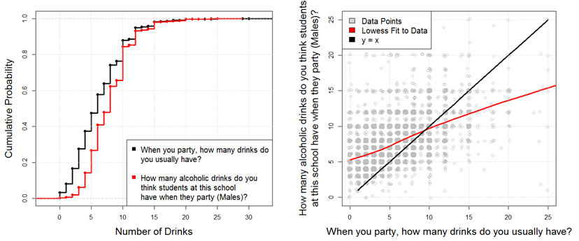
Figure 1. ECDF (left) and scatterplot (right) of the "number of drinks when you party" and "How many drinks do you think students at this school have when they party?"

2.4

As we can see from Figure 1, on the left, a comparison of the two distributions indicates that the distribution "How many alcoholic drinks do you think students at this school have when they party" is uniformly shifted to the right of the actual drinks students tend to consume. While not shown on the figure, this shift in distributions is observed among 31 of the 32 universities in the SNMRP sample. On the right, we plot perception of drinking versus actual drinking: each of the gray circle data points represents individual student drinking and opinion of the drinking of others. In the right panel, the reader should note that the actual survey data is ordered pairs of integers. Were we to plot integral values, the data points would obscure each other, so we have added a small amount of random noise to ("jittered") each data point so that the density can be more easily seen. In the right panel, we see that students that drink less than 10 drinks (approximately 85% of the population) tend to overestimate the level of drinking that occurs. While the variables are moderately correlated (Spearman rho=0.5260), it is clear that most of the data points are above the line y=x, indicating that most students have a tendency to over-perceive, with the exception of the heaviest drinkers in the population.

2.5

As mentioned previously, social norms theory suggests that perception of drinking behavior leads students to approximate that behavior (Berkowitz 2005). The scatterplot (right) of Figure 1 indicates a positive correlation between actual and perceived drinking levels, leading us to this question: "why is the perceived behavior not eventually attained?" If we consider a simple dynamical system in which drinking rates change in accordance with the discrepancy between the actual drinking level and the perceived norm, we might expect the actual drinking level to tend toward the perceived norm (Lapinski & Rimal 2005). Since the perceived norm remains higher, we are left wondering about the nature of the dynamics.

2.6

SNT in this form does not address the issue of dynamics. How individuals choose reference systems or groups to moderate individual behavior and how reference systems change remain to be resolved. In order to elaborate on the SNT model, we integrate some key insights from Identity Control Theory, a dynamic model of social interaction. Identity Control Theory provides a foundation that naturally allows the incorporation of misperception and the wa

2.9

y in which it enters drinking behavior dynamics.

Identity Control Theory

2.7

Identity Control Theory (ICT) states that identities are formed by a set of meanings that serve as a reference or standard for defining who one is (Burke 1991; Stets & Burke 2000; Burke & Stets 2009). An individual's self comprises a number of identities, any of which may be salient in a given context or situation (Stryker & Burke 2000). When an identity becomes salient in a social situation, the individual or agent perceives appraisals from others. If the appraisals are not in line with the agent's meanings, the agent experiences distress. This distress may lead to behavioral changes in the agent. Burke and Stets (2009) use the analogy of engineering feedback control systems that monitor inputs from their environments and apply control signals to bring the system outputs into agreement with a reference or tracking signal. Inputs are generally meant as direct or indirect social cues that are referred to as appraisals from agents in the social environment (Burke 1991), and the controls are an agent's behavior. A conceptual diagram of ICT (slightly adapted from Burke 1991) is provided in Figure 2.

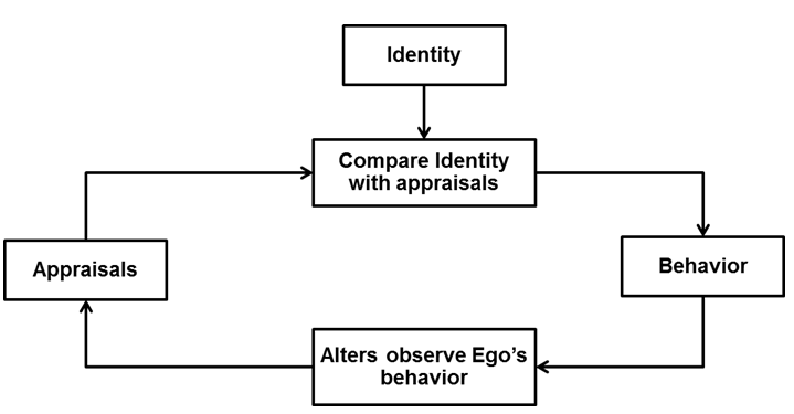
Figure 2. Block diagram of ICT appraisal processing and behavior adaptation.

2.8

All this is certainly not to say that humans operate exactly as an aircraft's flight control system or chemical plant's mixing reactor. As noted by Burke and Stets (2009), the control system is but one component of Identity Theory. Cognitive and emotional processes are also involved in identities, and conscious thought and action play vital roles in how we act and what we do. Humans also have multiple identities (e.g., father, student, activist, soccer enthusiast, waitress) with complex salience and prominence hierarchies suggesting which identities may become activated and which identities are preferred by the agent (Stryker 1968, 1980; McCall & Simmons 1966). The control system analogy serves here as a simple basis for constructing a small-scale computational society in which agents interact and modify their behaviors in response to interactions.

2.10

A brief illustration of the identity control process may serve to show how the model works. Consider "Joe," an 18 year old freshman in college. Joe wants to join the most exclusive fraternity on campus. This fraternity has the reputation of being hard drinkers. In order to join the fraternity, Joe develops a set of meanings of what it means to be a fraternity member. These meanings may define how he dresses, how he acts, who he socializes with, among other things. In addition, he also incorporates meanings that define what kind of drinker he should become. This drinker identity serves as a standard for his drinking behavior.

2.11

As Joe interacts with his friends, while consciously or not, he monitors the appraisals from his peers about his own drinking behavior. If the appraisals that he receives suggest that he is not drinking enough, then he consumes more alcohol. If those appraisals suggest that he is drinking too much, then he slows down his rate of consumption. The key notion here is that individuals monitor appraisals and adjust behavior so that the appraisals that he receives from his peers are consistent with how he sees himself. In essence, individuals modify their behaviors so that their identities are verified in their interaction encounters. We refer to this form of feedback control as Identity Verification (IV).

2.12

The "tracking error" in this control model is referred to as distress. Distress is a central concept in Identity Control Theory, since it is believed that individuals will modify their behaviors in order to reduce the distress, or the discrepancy between their identity standard (their set of meanings for that identity) and the inputs that they receive from their interaction partners.

2.13

We also note that, while modifying behavior to reduce distress is the simple control model we adopt here, other ways of coping with distress are possible. Another way is to change identity (Burke 2006; McFarland & Pals 2005), so that behavior and appraisals are consistent with the new identity standard. Alternatively, one can engage in selective interaction strategies by finding interaction partners that are more likely to verify an identity (Robinson & Smith-Lovin 1992). In the present model, we make the simplifying assumption that agents only reduce distress by modifying behavior.

2.14

Experimental evidence for this model includes the teamwork exercise to explore a "dominant person" identity (Swann & Hill 1982) and other laboratory and survey research (see, Burke and Stets 2009, and the references therein). Recent results of Stets and Burke (2014) suggest that distress reduction may contain some nonlinearities. The simplest computational interpretation of behavioral change to bring appraisals into agreement with identity meanings is a linear feedback of the distress, as measured by "appraisals minus meanings." Stets and Burke observed in experimental settings that when an identity implies positive and negative connotations (such as, being a good employee or being an "honest" person) appraisals that are more positive may lead to an enhancement effect of good feelings as well as the expected consistent effect of distress over unmatched feedback. What this experimental result suggests is that appraisals that "overshoot" an identity meaning may not lead to the same level of distress as appraisals that "undershoot." That is, an agent may work harder or faster on behavior to alleviate negative appraisal discrepancies than s/he would to reduce positive ones. In this regard we are most certainly simplifying the identity control process. Emotional and cognitive thought processes thus impact the control loop in ways we do not fully understand. With these caveats in mind, we take this first step in implementing ICT into a computer simulation of a college drinking event.

Peer Influence

2.15

ICT provides an important complementary process to classical Social Influence Theory (Abelson 1964; Friedkin & Johnsen 2011; Isenberg 1986; Mason et al. 2007). We consider in this work a peer influence (PI) model of social influence as a second form of feedback control of drinking behavior. The distinction from IV is that PI models a behavioral change in which individuals seek approval by adopting the behavior of others. Peer influence can encompass a number of control actions (Borsari & Carey 2001). Within the college drinking context, peer influence can range from direct offers of drinks to indirect modeling of others' behaviors to that of identity control. Indeed, ICT involves an element of peer influence, as peers provide appraisals that an individual processes to examine identity. Our PI model is the indirect sense of an individual attempting to model the behavior of peers, much like attitude and opinion dynamics of Abelson (1964). Indeed the simple feedback model we define below closely follows the dynamics of Abelson's attitude model. As noted in Borsari and Carey (2001), this indirect sense involves an individual matching the concurrent drinking of peers within the drinking event: past observations do not tend to enter into the control model. Moreover, this control behavior appears to be independent of the individual's awareness of the peer influence. Experiments (DeRicco & Garlington 1977; DeRicco 1978) have tended to corroborate the notion that agents are influenced by indirect PI within a drinking context. Osgood and colleagues (2013) also observe not only significant relationships between individual and peer behavior in alcohol use but also strong tendencies for friendship selection based on similar drinking behavior.

2.16

Together, the PI and IV models form our social influence model of drinking behavior, which is illustrated in Figure 3. It is interesting to note that IV and PI have different impacts on group, and hence aggregate, behavior. Both PI and IV affect the individual agent's behavior, but the agent's behavior becomes a component of the group behavior, which creates a loop back to the individual through the PI model.

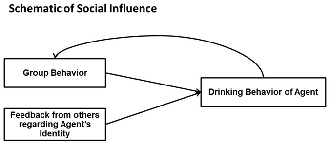
Figure 3. Drinking behavior adaptation from ICT appraisal feedback and peer influence.

2.17

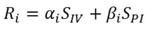
Together the IV process and the PI process can be applied to explain the drinking rate of the individuals. Figure 4 is a conceptual representation of how these two processes intermingle. Since individuals may weigh identity appraisals and the group influence differently, we suggest weighting factors (a and ß) that are used to define an agent's commitment to his/her drinker identity; that is, those agents that are highly committed to their drinker identity will weigh the appraisals that they receive more heavily than those that have a low commitment to their identity. The concept of commitment is an important component in the identity control process (Burke & Reitzes 1991). While the impact of social influence in the PI model is the act of modifying behavior to match the drinking rate of a person's peers, the form of influence that results from an interaction encounter results from a person's desire to meet verification needs.

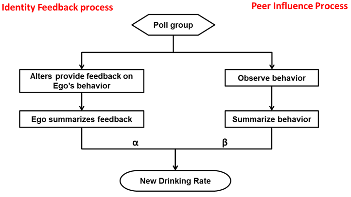
Figure 4. Adaptation of Identity Verification needs and Peer influence.

2.18

By focusing on drinking identities, we are of course abstracting the problem down from the many complex issues that make up a population of college students. Gender, ethnicity, socio-economic status (including parental educational attainment as well as income), and other identities all have impacts on a student's drinking behavior (Wechsler et al. 2002).

Interacting Groups at the Party

2.19

Generally speaking, party events do not involve a single large group of individuals who are simultaneously interacting with everyone else, nor do they involve singletons behaving as if alone. Rather, parties and social events tend to involve smaller clusters of interaction partners within the larger event (Bakeman & Beck 1974; Ingram & Morris 2007). One of the primary challenges with this particular aspect of the model is that little empirical research exists on how small groups form and break up at short-time social events such as parties. Interesting technical innovations (see, e.g., Cattuto et al. 2010; Setti et al. 2013) including Radio Frequency Identification (RFID) chips and computer vision systems offer new means of tracking groups and clustering at parties and other events, but empirical studies using these for social sciences purposes are quite few. A number of more mathematical approaches (Kelly 2011; Wilenski 1997) have also been developed.

2.20

There is, on the other hand, a great deal of empirical research on many aspects of the evolution of groups and of social networks and their dynamics. Much of this work is focused on a longer time-scale than is at issue for a single party or drinking event, but the network structure and dynamics provide some insight into friendship networks. The Framingham Heart Study Social Network (see Christakis & Fowler 2007; Rosenquist et al. 2010) shows the importance of friendship ties in health behaviors over a long time period, wherein a "three degree of separation" emerges as a strong indicator of related behaviors. Rosenquist et al. (2010) note that both social network and interpersonal effects are important in alcohol consumption behaviors and observe that social network effects may have both positive and negative impacts on drinking behavior, a result in line with the IV and PI components of our model.

2.21

We should note that there are interesting longer term effects of the interplay between drinking behavior, friendships, and groups, which are not modeled in the present work. Our short-time model of an individual drinking event involves a group formation dynamic based on a friendship network and trait similarity (homophily) which is not correlated with drinking rates. Osgood et al (2013) demonstrates correlations between drinking rates and interaction partners. Over time, we might expect a learning process to engage, in which agents modify their friendship networks based on similar drinking behavior as well as trait similarity. Modeling this more complex longer term process may be rather challenging: Shalizi and Thomas (2011) note teasing out the causality of events arising from homophily and social influence is quite difficult.

A Simulation Model of a Drinking Event

3.1

A single college drinking event ("party" hereafter) can range from a few friends meeting up in a dorm room to a large party hosted by a Greek organization (fraternities or sororities, which are social organizations common to US universities) to a pre- or post-game gathering around a large sporting event. The basic properties we take for a party include a number of participants (agents), access to alcohol, and a limited duration for the party. During the party, agents form groups dynamically, and individuals may depart to join other groups or split along with others to form new groups. Friendships and trait similarities govern the manner in which groups form and break apart. Also during the party, individuals consume alcohol based on the feedback models of ICT and PI.

3.2

The party operates with a pre-determined number of agents, N, and for a pre-determined number of hours, H. We run a discrete time simulation with a fixed clock ticking every ?t hours. A drink is the so-called "standard drink," which contains 10 grams of ethanol, approximating the rule of thumb that one beer equals one glass of wine equals one shot of liquor. During the party, as noted above, the agents consider their groups and their drinking rates.

3.3

A few primary processes are needed to instantiate the agents and implement their behaviors in a simulation.

1. Agents assort themselves into interacting groups. For this simple model, a friendship network and a trait attribute are used to simulate the dynamics of grouping together and breaking apart. Agents assess their similarity in terms of friendships and traits with members of groups to decide whether to remain in a group or move on to another. The grouping governs the interaction partnerships, which in turn govern the drinking signals.
2. Agents observe the drinking in the group. This indirect PI process contributes to the agent's decisions on how much to drink.
3. Agents give to and receive from members of their group appraisals about drinking behavior. Drinking behavior is an identity, instantiated as a categorical drinker type. Each agent attaches a quantitative drinking rate "meaning" to each drinking identity type, and the appraisals an individual receives are coded as these drinking rate meanings. These IV appraisals also contribute to an agent's decisions on how much to drink.

3.4

Three key parameterizations are involved in the drinking processes (B) and (C):

1. Each agent weights the IV (C) and PI (B) drinking rate information to make a decision concerning her/his drinking rate. We denote these weights by a and ß respectively.
2. Each agent has an identity, which is a qualitative categorical symbol of her/his drinker type. Associated with this identity, the agent has a meaning that denotes an actual numerical drinking rate that the agent connects to her/his identity.
3. Each agent has a set of meanings that s/he attaches to each the identity types as s/he perceives them to apply to others. These meanings are actual numerical drinking rates for each identity type. In view of SNT's ideas related to misperception, these identity meanings (which form the basis of appraisals the agent will provide to others) may be positively biased away from "truth" (which we infer from SNMRP survey responses).

3.5

Before drilling down into the group and drinking blocks, we describe the agent attributes needed to model the dynamics.

Agent Attributes and Model Parameters

3.6

Agents in the model are relatively simple actors with a small number of attributes. We delineate them below. A number of attributes are random quantities whose distribution models require some flexibility. We will discuss those details when we specify parameter values and provide simulation examples in Section 4. Modeling the dynamic process also requires the selection of functional forms for a number of decision computations. As is often the case in agent-based modeling of social systems, we have little in the way of hard data to choose these forms, and here we make selections based on directionality (do the relationships go in the right direction?) and simplicity.

1. Agent ID number: we assign each agent a unique number ID_i from 1 to N, where N is the number of agents attending the party.
2. Agent trait: each agent is assigned a random trait T_i from a uniform distribution on the interval [0,1]. This quantity is an abstract trait meant to provide a means of agents finding other agents with similar interests for the grouping process (A).
3. Agent drinking identity: each agent is randomly assigned a category D_i, one of the five drinking types. The likelihoods of the five types are specified as a simple probability mass function, and this distribution is flexible. This attribute determines the agent's identity as in (C).
4. Agent identity definitions: for an agent to define his/her identity and to provide appraisals to others, the agent must have an idea of what level of drinking is compatible with each type. Each agent is assigned five drinking level perceptions, R¹_i, R²_i, R³_i, R⁴_i, R⁵_i, one for each category. These levels are drawn from lognormal distributions (this distribution is discussed more below) whose parameters are flexible. The agent sets as R^*_i the drinking level from these five levels that corresponds to his/her identity. This attribute provides the meaning an agent attaches to her/his identity (and in the absence of SNT misperception to the identities of others). These numbers provide simple, specific meanings to the identities as in (C).
5. Agent identity misperception: the parameter e^j_i = 0, j=1,2, …, 5 is added to the identity definitions R_i^j as a means to model SNT misperception. This parameter may be set to 0 or sampled from one of a choice of distributions. The use of a non-negative misperception derives from empirical research (see, e.g., Borsari & Carey 2003).
6. Agent appraisal feedback: the parameter F^j_i = R^j_i + e^j_i is the appraisal agent i provides to group members of the 5 drinking identity types. These quantities are not independent attributes: rather they are determined directly from attributes 4 and 5. It is an important feature of the model that an agent may provide higher appraisal feedback to others than s/he might expect for him/herself. These feedback appraisal drinking rates are the meanings an agent attaches to the identities of other agents.
7. Agent commitment to identity: a number a_i between 0 and 1 is assigned to each agent, governing (as described in Subsection 3.3 below) how strongly the agent responds to appraisal feedback on identity, relating to (C) above. How much of an agent's drinking rate is based on IV is governed by this parameter. The assigning distribution is flexible.
8. Agent responsiveness to peer pressure: a number ß_i between 0 and 1 is assigned to each agent, governing (as described in Subsection 3.3 below) how strongly the agent responds to peer pressure to conform to the group drinking rate, relating to (B) above. We require a_i + ß_i = 1 for each agent. How much of an agent's drinking rate is based on IV is governed by this parameter.
9. Friendship network: encoded as an array (called an adjacency matrix), C_ij with indices denoting two agent ID numbers, the friendship network is defined by C_ij = 1 when agents i and j are friends and 0 if they are not. This matrix is undirected. This may be initialized as 0 for a freshman mixer model or any other network construct. The friendship network impacts the dynamics of groups as in (A) above.

3.7

With the individual agent attributes in hand, we define parameters and model functions that are fixed for all the agents for the party simulation.

10. Size of party: N is the number of agents attending the party.

11. Duration: H is the party duration in hours.

12. Time step: ?t is the time step in hours at which simulated actions are taken.

13. Group similarity model parameters: to determine an agent's "fit" within a group, Agent i computes the dynamic quantity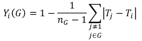

(1)

for each group G (with i added to G if i is not a member). This quantity is the trait similarity score for Agent i, which in turn becomes the overall similarity score

(2)

In Equations (1) and (2), we use the following notation: T_k denotes the trait of Agent k; n is the number of individuals in the group; F_pop is the fraction of the population that the agents have identified as friends (this is a vector); and F_i = F_i (G) is the fraction of the group that the agents have identified as friends (also a vector). Equation (1) provides a simple trait-discrepancy based score for how well the agent fits into a group. The similarity score of Equation (2) allows the agent to weight friendships and trait similarity. If the agent has few friends at the party as a whole, then the agent is more attracted to a group containing friends. If the agent has many friends at the party, the agent becomes more likely to seek groups of individuals with similar traits.

14. The probability of departing a group due to dissimilarity is the dynamic quantity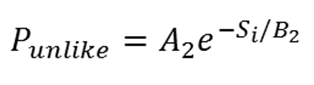

(3)

For the purposes of the simulation, we set A₂ = 0.6, B₂ = 0.15. Equation (3) provides a simple functional form to the idea that as the similarity score increases, the individual becomes more likely to leave the group in search of another.

15. Group entropy model parameters: groups may split up from "entropy" as well as dissimilarity. The model is a probability of departing that depends on group size: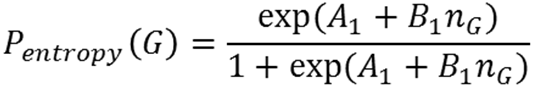

(4)

in which the dynamic quantity n_g denotes the number of individuals in the group, and the constants are set as A₁ = -7.00, B₁ = 0.50. Equation (4) provides a simple functional form that increases and saturates with the number of individuals in the group.

16. Identity appraisal statistic: each individual receives appraisals from group members concerning the drinking rate deemed appropriate for the individual's identity. The agent forms a statistic S_IV, which may be set as the median, the mean, or a weighted average of the feedback appraisals the agent receives from the other members of the group. The statistic can be flexibly selected but takes the same functional form for all agents.

17. Peer influence statistic: each individual observes the drinking rates of the group members. The agent forms a statistic S_PI, which may be set as the median, the mean, a weighted average, or the maximum, of the rates of the other group members. The statistic can be flexibly selected but takes the same functional form for all agents.

18. Blood Alcohol Content (BAC) statistic: as a simple means of introducing a reasonable upper bound on consumption, we use Widmark's function (Snyder 1992) for BAC in terms of drinks (D) and the elapsed time in hours since consumption (h):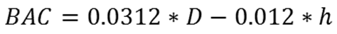

(5)

The constants are empirically determined (and in general depend on body mass and gender, Snyder 1992). Individuals pass out at a BAC of 0.30 and die at a BAC of 0.40.

The Group Formation Model

3.8

As agents enter the party, they form into groups. The process of grouping is illustrated in the flow diagram of Figure 5.

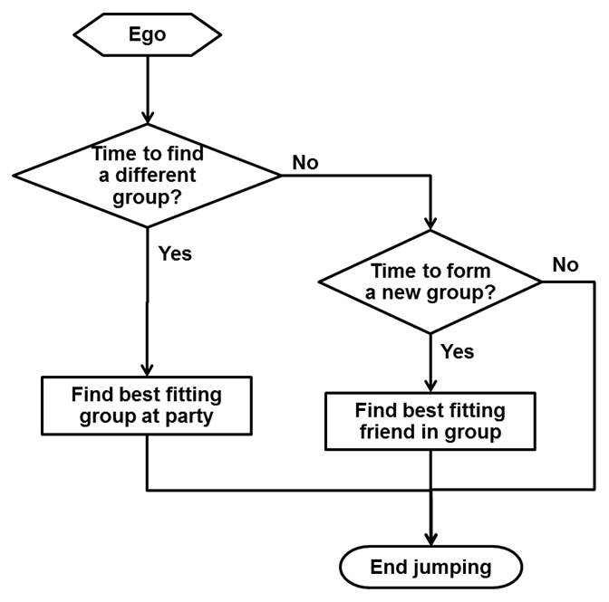
Figure 5. Block diagram of group formation.

3.9

We outline the process as follows. At a given simulation time step, we perform the following operations.

1. Loop through the agents in randomized order to select the "ego" agent.
2. Compute trait similarity score for the current group and other groups.
3. If there is a better group, jump to that one with probability P_unlike.
4. Compute the entropy probability and depart with closest trait similarity scoring group member to form a new two person group with that probability.

After the agents consider their peers in this group formation model, they consider their drinking rates.

The Drinking Model

3.10

The drinking model has agents consuming alcohol in terms of standard drinks over the party duration. The rate at which agents consume will impact their BAC and hence their basic state of being active, passed out, or deceased. In the end, the model's primary output is the number of standard drinks each student has consumed. The process of drinking is illustrated with a block diagram in Figure 6.

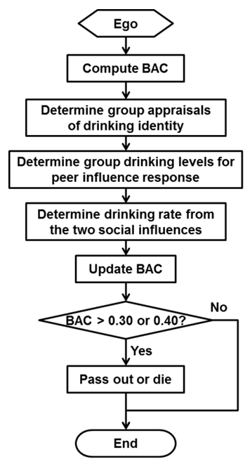
Figure 6. Drinking Component

3.11

We outline the process as follows. At a given simulation time step, we perform the following operations.

1. Loop through the agents in randomized order to select the "ego" agent.
2. Compute the statistic S_PI for the members of ego's group.
3. Compute the statistic S_IV from the members of ego's group.
4. Compute ego's new drinking rate:

   (6)

Having checked for groups and adjusted the drinks, the time step is complete. 1. 2. 3. 3.1. 3.2. 3.3.

The Friendship Formation Model

3.12

As agents participate in groups, they may encounter other agents they do not directly know either entering a new group or staying with a group that gains new participants. In this module, agents that were selected to consider jumping will loop through the members in their group for the possibility of gaining new friends. In our simple model, we use the trait attribute to model similarity for the purposes of friendship. If two individuals i and j are not friends, then the agent will compute how similar the two agents are with respect to their traits values: pairwise trait similarity between agents i and j is U_i,j = 1- |T_i - T_j|, where T_i and T_j correspond to the trait values of agents Ego and Alter. The probability that these two agents would become friends is given by the following logistic function:

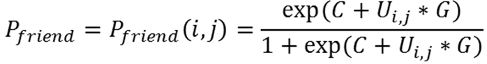
(7)

where C and G are numeric constants set to -5 and 2. We choose the logistic as a model for the "befriending" decision due to its simple functional form, increasing with horizontal asymptotes at 0 to the left and 1to the right.

3.13

We note that, in this simple model of a dynamic friendship network, friendships form but do not break. We also note that the formation of new friendships will have an impact on group assessments and dynamics. That is, when an agent considers a decision to remain in her/his current group or move to another group, that agent's friendship network plays an important role.

The Simulation Model "At A Glance"

3.14

We close this section by summarizing the model in a list of computational steps, integrating the attribute and dynamic blocks into a single procedural outline.

1. Initialize the event, by choosing the time duration and the number of agents.
2. Initialize the agent population:

1. Assign each agent a trait variable from a uniform distribution.
2. Assign each agent an identity from a discrete distribution of identity types, namely abstainer, infrequent, light, moderate, or heavy.
3. Assign each agent an identity meaning, which is a drinking rate, from a lognormal distribution associated with the agent's identity type.
4. Assign each agent five identity meanings to be used when providing feedback appraisals to other agents.
5. Assign each agent commitment levels (a and ß) to IV and PI processes, from uniform distributions (and normalized to sum to 1).
6. Build an initial friendship network as a random graph.

3. Loop over time to allow the event to run. At each time step

1. Check the grouping. Agents will decide (with probability from Equation 3) to consider moving to another group. If a "considering" agent finds a group that has higher similarity (as determined by Equation 2), then the agent may join that group. If a considering agent does not find a higher similarity group, that agent may (with probability determined by Equation 4) decide to take a friend in the current group and split off into a new group.
2. Check friendships. Agents who have considered moving to a new group will also examine individuals with whom they are not currently friends. The "considering" agent will add not-current-friends to their friendship network with a probability that depends on trait similarity, from Equation (7).
3. Check the drinking. Agents will decide (at a random rate) to consider drinking more. The "considering" agent will obtain appraisals from group members and observe the drinking rates of group members, forming a new drinking rate according to Equation (6). The agent will then check BAC from Equation (5).

4. When the time loop of Step (3) completes, the party is over.

3.15

We move now to running the simulation to investigate the effects of misperception, social influence, and identity control on aggregate drinking outcomes.

Simulation Analysis

4.1

Having discussed the model's design and parameterization, we conduct a suite of simulation studies to investigate the collective behavior of students drinking at a party. As noted above, there are a number of parameters relating to the IV and PI modeling. The impact of these model specifications on the system is of great interest, both for the design of surveys and other data collection efforts and the development of policy actions that may mitigate problem outcomes.

Parameter Specification

4.2

For the purposes of this exposition, we simulate the behavior of N = 20 students at a party of duration H = 4 hours under a number of parametric configurations. A number of parameters defined in the Agent Attributes and Model Parameters section as "flexible" need to be specified.

4.3

First, the proportions of agents in each identity type are given in Table 1. The identity labels are taken from Wechsler et al. (2002), and the proportion values are loosely based on the CAS results described therein. Respondents to the CAS were asked to self-identify as one of seven types (these five plus Abstainer-in-Recovery and Problem Drinker). It is important to note that students were not given definitions of these terms: rather, the respondents chose the term felt to be most self-descriptive.

Table 1: Probabilities of agents being assigned to each drinking identity
Drinking Type	Proportion
Abstainer ~ D1 Infrequent ~ D2 Light ~ D3 Moderate ~ D4 Heavy ~ D5	0.1697 0.3138 0.2255 0.2477 0.0433

4.4

Second, the drinking levels for each of these five types are specified in Table 2. In order to assign a level of drinking to each of these identities, we examined the number of drinks consumed at a drinking event by individuals who self-identified in each of the five types in the CAS survey. From these data we obtain five probability distributions to model the individual drinking levels. Thus, we tie these self-selected identity terms to the amount the individual is likely to consume at a drinking event. The lognormal distributional form we use to fit these data is commonly used for modeling drinking rates (see, e.g., Ledermann 1956; Skog 1985; Nahas et al. 1999). The choice of the lognormal relates to the nonnegative, left skew, relatively long tail behavior it exhibits that is typically seen in observations of drinking rates across a population. Figure 7 shows the lognormal densities having these parameter specifications.

Table 2: Parameters for drinking rates for each of the five identities
Drinking Type	Lognormal Mean	Lognormal Standard Deviation	Mean Drinks/Event	Standard Deviation Drinks/Event
Abstainer Infrequent Light Moderate Heavy	-4.6874 0.1830 0.9770 1.4895 1.9035	2.0224 0.9031 0.5213 0.4067 0.2536	0.0712 1.8054 3.0431 4.8172 6.9286	0.5457 2.0270 1.7005 2.0431 1.7857

4.5

For the IV agent identity misperception, we consider three cases: e = 0 (no misperception), e lognormally distributed with mean 0.5 and variance 1.0, and e lognormally distributed with mean 1.0 and variance 1.0.

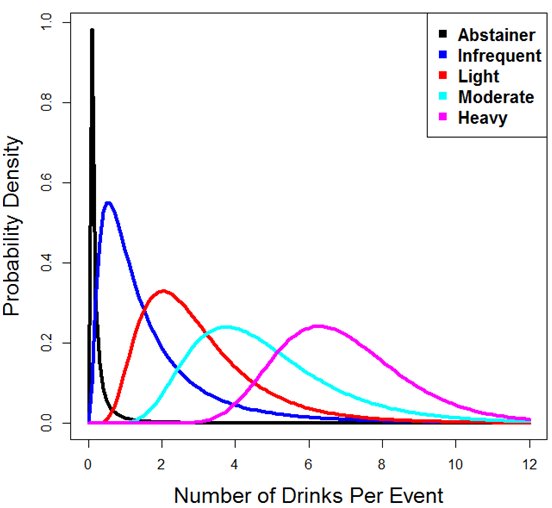
Figure 7. Modeled drinking level likelihoods for the five drinking types

4.6

We note here that a heavy episodic or binge identity is not specifically part of the model. With the standard definition of heavy episodic drinking being five or more drinks in a single event period for men, we see that even self-identified abstainers have some chance of becoming bingers, while moderate and heavy drinking identities are quite likely to undertake binging behavior.

4.7

For agent commitment to identity (a) and responsiveness to peer influence (ß), we consider three cases. We set a₀ = 0.20, 0.50, or 0.80 and ß_{0 =}1- a₀, and for each agent we generate a pair of uniform random numbers (a', ß') on (0, a₀), (0, ß₀) respectively. Finally these pairs must be normalized to sum to one, so we set a = a'/(a'+ ß'), ß = ß'/( a'+ ß'). Figure 8 illustrates the resulting distribution for a based on this process, for a₀ = 0.20, 0.50, or 0.80, as well as the expected value of a (after the normalization). A simpler modeling choice would be to model a with a uniform on [0, a₀] and take ß₌1- a. The slightly unusual choice we have made still allows the population of agents to have a full spectrum of (a, ß) pairs between 0 and 1 but with bias in one direction or the other depending on a₀.

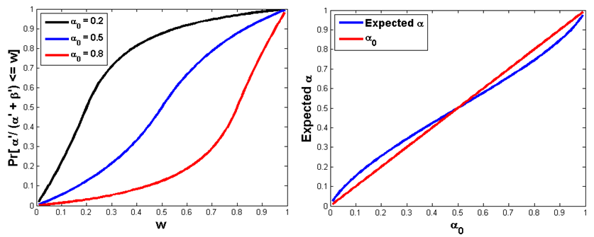
Figure 8. ECDF of a (left panel) and expected a (right panel)

4.8

We have now fully specified the model's functional forms and parameters so that simulations can be executed. Table 3 summarizes the 3×4 factorial design of this study. As previously mentioned, we have 3 levels of the a₀ conditions (0.20, 0.50, 0.80), and we have four levels of the misperception condition. Table 3 summarizes the structure of the model, and follows our inquiry into investigating sources of influence on agent behaviors. The a₀ conditions define the distributions of agents' commitment levels to their drinking identities and of their responsiveness to peer pressure. As can be seen in Figure 8, the low choice of a₀ =0.20 leads to a population of agents that are highly susceptible to peer influence, while the higher choice of a₀ =0.80 leads to a population of agents that drink at a rate that matches their identity verification needs. The second factor in the analysis involves the different forms of misperceptions (either biased appraisals or different group conditions) and their effect on drinking behavior.

Table 3: Experimental conditions for our simulation study
High a0=0.8	Medium a0=0.5	Low a0=0.2
e = 0, group median e = 0, group max e ~ LogNorm(0.5,1), group median e ~ LogNorm(1.0,1), group median	e = 0, group median e = 0, group max e ~ LogNorm(0.5,1), group median e ~ LogNorm(1.0,1), group median	e = 0, group median e = 0, group max e ~ LogNorm(0.5,1), group median e ~ LogNorm(1.0,1), group median

4.9

For each of these 12 conditions, we simulate 10,000 Monte Carlo realizations. In the following subsections, we discuss different aspects of the model output.

Illustration of Simulation Dynamics

4.10

For illustration purposes, we have selected our baseline model of a₀ = ß₀ = 0.50, with e=0/group median for the feedback statistics agents use to adjust their drinking rates. In the following figures, we present the network dynamics of group jumping, group sizes, the drinking behavior of agents over time.

4.11

Figures 9–12 provide a glimpse into the behavior of agents at the parties, for two realizations of the model simulation. In Figure 9, the left panel contains the initial simulation state. The panel on the right contains the final state at the end of the simulation. The circles denote the agents, with the line segments denoting the friendship network. Numbers on the agents denote the drinks consumed, and colors denote the group membership. Figure 10 provides an animated GIF of the 20 partiers as they group together, separate, and drink, starting from the left graph illustration of Figure 9 and ending at the right. Figures 11 and 12 are identical in concept to 9 and 10 but illustrate a different realization.

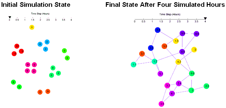
Figure 9. Initial State and Final State of one Realization. Example 1.

Figure 10. Animation of Network evolving #1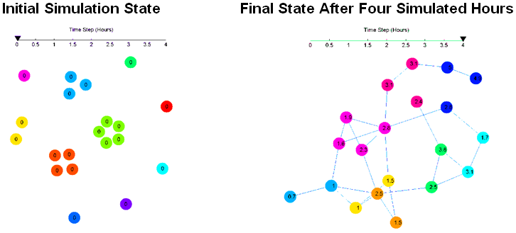

Figure 11. Initial State and Final State of one Realization

Figure 12. Animation of Network evolving #2

4.12

Statistics of the grouping process are recorded in Figure 13 and 14, for 1,000 realizations of the model simulation. In Figure 13, we present an image plot of the group size for all time steps in the model. At the bottom of the figure (along the x-axis), we present time in units of hours (for a 4 hour party). Along the y-axis, we observe the size of the group. The colors in the figure denote the fraction of each group size in the population. The black line in the figure denotes the median group size for those realizations. Moving from left to right in the figure, we observe that group size starts out fairly small (around 4), increases dramatically (up to 6), but decreases to a median of size 3. We also notice that the variance of group size also decreases. At the fourth hour, the distribution is positively skewed as noted by the dramatic change in color intensity between group sizes 2 and 3 along the y-axis, and the gradual change in color values from group sizes 3 to 7. In Figure 14, we present animation of these processes over the course of the party.

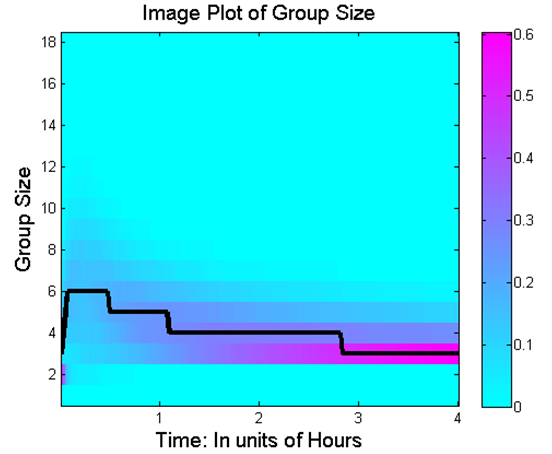
Figure 13. Distribution of group size as a function of time. Black line in the figure denotes the median group size for each time step. The cyan and magenta color intensities denote the proportion of the population for each group size.

Figure 14. Animation of Median Group Size and Histogram of Group Size as a function of time

4.13

In Figure 15, we observe an animation of the proportion of group departures for one thousand independent simulations. That is, how many times do agents jump to new groups or form new groups during the course of a party? In the top panel of the figure, we see the median number of departures for all 1000 simulations. The bottom panel of the figure provides a histogram of the jumping behavior as it changes through the course of the simulation. The animation illustrates that initially agents make many departures quickly; however, after a while they have a tendency to find individuals in groups that they get along with. Also, in the bottom panel of the figure, we observe a histogram of the jumping frequencies. The variance of the distribution appears to increase as 'outliers' (i.e., agents with no friends) make last ditch efforts to find suitable interaction partners at the party.

Figure 15. Animation of Median Group Departures and Histogram of Group Departures as a function of time

4.14

Figure 16 contains an animation of the kernel density estimate of the number of drinks consumed, computed for 1000 realizations. The top portion of the figure contains the drinking rates of those agents at the first, second, and third quartiles of the drinks distribution, as it varies over time. As observed in the animation, agents ramp up their drinking behavior to catch up with the appraisals and peer influence models. However, after an hour of drinking their drinking rates slow down. It is also important to note that this time period is the most active time period in the model. This is where most of the group departures occur and where the variation in group size tends to be the largest.

Figure 16. Animation of Drinks. Top Panel: The first, Second, and Third Quartile of Drinking Rates as a function of time. Bottom Panel: The Kernel Density Estimate of the Number of Drinks consumed

4.15

Those agents that are at the first quartile appear to settle into an equilibrium after three hours, while those agents at the second and third quartiles appear to continue to slightly increase their rate of consumption.

4.16

These images and animations provide a nice visual sense of the simulation's operation. Using the model for scientific and policy inquiry is the topic of the next subsection, wherein we examine the full 10,000 realizations for each of the 12 experimental conditions of Table 3.

4.17

Again we note that a paucity of quantitative empirical data on dynamic grouping in a social environment makes it difficult to validate the model. However, qualitatively this data appears to match observed video data of mixing at parties (Setti et al. 2013), and quantitatively the group size data compares well to related observational data (Bakeman & Beck 1974). Figure 17 compares the cumulative distributions of our simulation with two sets of data presented in Bakeman and Beck (1974).

Figure 17. Comparison of simulated group sizes with observed grouping behavior from Bakeman & Beck (1974).

Analysis of the Simulated Drinking Data

4.18

We begin our analysis with the aggregate drinking behavior of the population at the end of the party. In Figure 18, we see the ECDFs of all 12 experimental conditions. Each of the four panels in the figure is conditioned on the misperception settings, while the data contained within each panel compares the a₀, ß₀ settings. The black line on all figures called "identity" is how much the agents would consume in the absence of any influence whatsoever. One can view this curve as the drinking behavior that would arise from agents drinking alone for 4 hours according to their drinking identities. Mathematically, this curve is the mixture distribution of the lognormals of Figure 7 with mixing proportions from Table 1. As observed from these data, we notice that alpha has a large effect on drinking behavior when e=0 and PI equals the max (top right of the figure). However, for the remaining models, the effect of the a₀,ß₀ settings are small but consistently ordered from less drinking when a₀ is high to more drinking when a₀ is low. Further, we observe a slight reduction in variance of each distribution as a₀ decreases.

4.19

We also note that the e=0/group median condition, our baseline model without misperception, is uniformly shifted to the right of the identity distribution. This curious result is explainable: agents' movements among groups have consequences for drinking behavior. In short, as agents seek to have their identities verified, they are faced with one of two choices. If their appraisals cause them to drink more, then the agents will consume more alcohol. However, when they are given appraisals that tell them they are drinking too much, they may only refrain from drinking. Since it is not possible to undrink, agents must wait for time to pass for their identities to be verified in those interaction encounters that suggest the agents have had too much. Therefore, modifying behavior in order to achieve identity verification (by multiple group members) leads to an effect comparable to a running max of appraisals. A running max of n+1 independent lognormals for different values of n is illustrated in Figure 19. If agents were to drink alone, then their drinking behavior would match the identity distribution. As we can see, taking the max of 2 appraisals leads to a median 1 additional drink over the four hour period, and the max of 8 appraisals will bring about 3 additional drinks at the median.

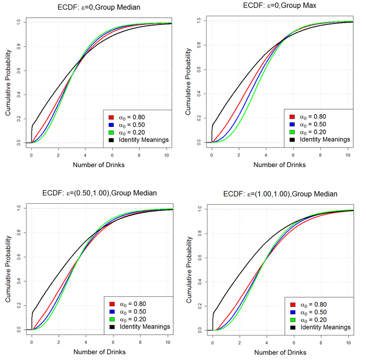
Figure 18. Comparison of ECDFs for each Influence Condition: No Misperception, e=0, Group Medium (top left); Group Misperception e=0,Group Max (top right); Moderate Identity Misperception e=(0.50,1.00), group Median (bottom left); High Identity Misperception e=(1.00,1.00), group Median (bottom right)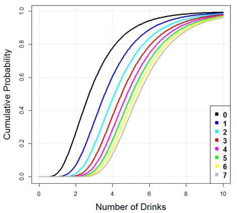

Figure 19. Running max of n+1 lognormals, n=0,1,…,7.

4.20

In Figure 20, we reorient the graphs in terms of the experimental conditions, organizing the plots by the a₀, ß₀ settings. In these figures, we can see how each misperception condition varies as a function of a₀, ß_0. Also particularly noteworthy, is that when a₀= 0.80, the e = 0/group max condition and the e = (0.50,1.00)/group median condition behave similarly. However, when a₀ =0.50 the effect of the group max condition is just as influential as the e = (1.00,1.00)/group median condition. And when a₀ = 0.20, the drinking behavior of the agents under the e = 0/group max condition exceeds the identity misperception condition e = (1.00,1.00)/group median.

4.21

As an additional parametric sensitivity study, we considered the impact of the initial friendship network. All of the simulations to this point were conducted as if at a freshman mixer, with no friendship ties at the onset of the event. We consider two straightforward modifications of this parameter setting. In one, we initialize the friendship network by setting all agents with trait differences less than 0.05 to be friends ("some friends initially"). In a second perturbation, we initialize the friendship network to be fully connected ("all friends initially"). In Figure 21, we see that knowing more people at the onset of the event reduces drinking slightly, a result nearly entirely due to the reduced movement from group to group that results from knowing more people.

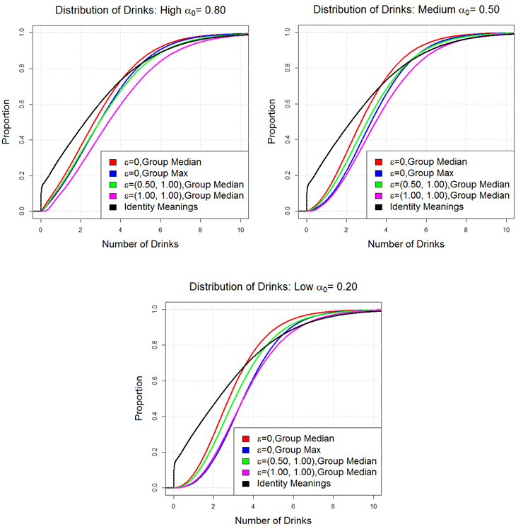
Figure 20. Comparison of ECDFs for each alpha condition: High (top left), Medium (top right), Low (bottom)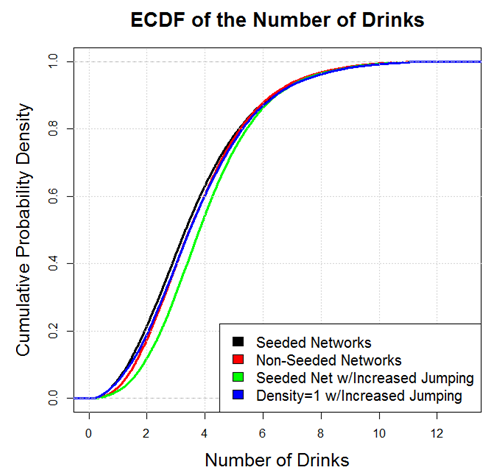

Figure 21. Dependence of drinking activity on initial friendship network.

4.22

The ECDFs in Figures 18 and 20 show a slight variance reduction at the macro level due to the decrease in a₀ and resulting increase in the impact of peer influence. In order to understand better the impact of the group on drinking behavior, we consider the intraclass correlation coefficient (ICC), a measure of the extent to which observations of units in the same group match (Sokal & Roholf 1995). In the large sample limit, the ICC can be viewed as the proportion of variance attributable to variation between groups. Thus, small values of the ICC indicate that variability within a group is comparable to variability between groups, whereas large ICC suggests that within group variability is small relative to the population's variability as a whole.

4.23

In Table 4, we examine the drinking data in terms of grouping. We present ICCs for the 12 simulation settings. The ICC allows us to assess how similar the drinking behavior is within the small groups that form during the party. As observed in Table 4, the ICC increases as a₀ decreases. The trend is to be expected, in that smaller a₀ means agents emphasize peer behavior matching in their drinking rates (see Equation 6), but the strength of the effect is quite remarkable for low a₀, corresponding to stronger peer influence, which pulls quite hard on the individuals to drink similarly to their group members.

Table 4: Intraclass correlation coefficient of Log Drinks within groups
a0	e = 0, Group Median	e = 0, Group Max	e ~ lN(0.50, 1.00), Group Median	e ~ lN(1.00, 1.00), Group Median
0.80	0.35	0.30	0.35	0.37
0.50	0.61	0.54	0.63	0.65
0.20	0.83	0.77	0.84	0.86

4.24

To investigate the results of our 12 simulation studies more deeply, we apply a hierarchical linear statistical model (HLM), using the number of drinks as the dependent variable, with individual identity, number of jumps from groups, individual a, and an identity*a interaction term as the independents. The hierarchy in the model arises from the formation of small groups, essentially a random effect that impacts the individual behavior. Membership in groups is an important effect for the inference, as the group members provide appraisal feedback and offer peer influence, and these dynamics create a within-group effect as is seen in Table 4. To integrate group membership into the inference, we note that while agents are joining groups at all times during the simulation, the agents have a tendency to settle into relatively stable social structures towards the end of the four hour period. Therefore, we use the group that the agent was in at the last time step to define a random effect term in the hierarchical linear model.

4.25

Our regression model takes the form

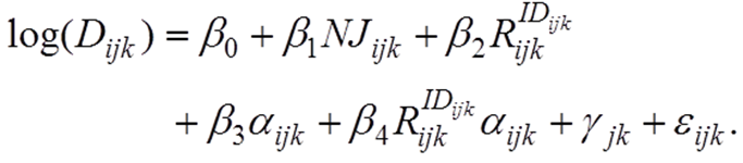
(8)

In Equation 8, the five regression coefficients, ß₀, ß₁, ß₂, ß₃, ß₄, relating the dependent log-drink variable to the independents, are given in Table 5 for each of the 12 different simulation settings. We use D_ijk, NJ_ijk, ID_ijk, R ^IDijk _ijk, a_ijk, to denote the number of drinks, number of jumps, identity type, identity meaning, and a value (respectively) for the i^th member of the j^th group in Monte Carlo realization k. The mixed-effects hierarchical variable ?_jk is a zero-mean random quantity modeling dependence of the log-drink variable on group membership in group j in Monte Carlo realization k. Finally, e_ijk denotes independent identically distributed zero-mean random errors. The number of groups and the number of agents in each group vary randomly within each Monte Carlo realization. Even though the indexing may suggest a three-level model, we are really modeling only two levels of hierarchy, with agents embedded in groups at a party, and Monte Carlo realizations provide replicate samples.

4.26

In order to compare the resulting coefficients across the 12 simulation settings, we have scaled the independent variables to standard normal units prior to conducting the regression analysis. We have also removed those agents that passed out or died. Table 5 contains results from this inference, indicating the five estimated regression coefficients (and their standard errors in parentheses) for the 12 distinct simulation experimental conditions. All coefficients are significant at the p < 0.001 level of significance. The extremely small p-values are due in part to the number of Monte Carlo simulations that we conducted.

Table 5: HLM Results for log drinks: standardized coefficients
a0		e = 0, Group Median		e = 0, Group Max		e ~ lN(0.50, 1.00), Group Median		e ~ lN(1.00, 1.00), Group Median
0.20	Intercept	0.9215	(0.0020)	1.1474	(0.0017)	1.0281	(0.0019)	1.1754	(0.0018)
	# jumps	0.0199	(0.0006)	0.0115	(0.0005)	0.0178	(0.0006)	0.0155	(0.0005)
	Identity Meanings	0.1345	(0.0005)	0.1093	(0.0005)	0.1276	(0.0005)	0.1126	(0.0004)
	a	-0.0749	(0.0005)	-0.1225	(0.0005)	-0.0691	(0.0005)	-0.0539	(0.0004)
	Identity meanings*a	0.1314	(0.0005)	0.1291	(0.0005)	0.1190	(0.0005)	0.0953	(0.0004)
0.50	Intercept	0.8712	(0.0018)	1.0447	(0.0016)	0.9826	(0.0018)	1.1421	(0.0016)
	# jumps	0.0278	(0.0010)	0.0236	(0.0009)	0.0260	(0.0009)	0.0191	(0.0008)
	Identity Meanings	0.3230	(0.0009)	0.2709	(0.0008)	0.3021	(0.0008)	0.2618	(0.0007)
	a	-0.1116	(0.0009)	-0.1681	(0.0008)	-0.1027	(0.0008)	-0.0781	(0.0007)
	Identity meanings*a	0.2020	(0.0009)	0.1909	(0.0008)	0.1780	(0.0008)	0.1376	(0.0007)
0.80	Intercept	0.7573	(0.0016)	0.8692	(0.0015)	0.8788	(0.0015)	1.0706	(0.0013)
	# jumps	0.0354	(0.0013)	0.0369	(0.0012)	0.0311	(0.0012)	0.0242	(0.0011)
	Identity Meanings	0.6431	(0.0013)	0.5696	(0.0012)	0.5937	(0.0012)	0.4965	(0.0010)
	a	-0.1308	(0.0013)	-0.1872	(0.0012)	-0.1137	(0.0012)	-0.0819	(0.0010)
	Identity meanings*a	0.2465	(0.0013)	0.2418	(0.0012)	0.2116	(0.0012)	0.1561	(0.0010)
* all coefficients are significant at p <0.001.
** Independent variables are in standard normal units.
*** Standard Errors are in parentheses.
**** Agents that passed out or died are removed from the regression results.

4.27

In these linear models, we observe that the number of jumps is positively associated with more drinking. This appears to be the result of the 'running max' phenomenon that is observed when agents interact with new interaction partners in the course of a drinking event. We also observe an interaction between "identity meanings" and an agent's a (i.e., commitment to their identity). When his identity meaning is a high drinking rate (high rate identity) and when he has a strong commitment to his identity, then the agent will consume more (on average) than someone with a lower commitment to his identity. Similarly, an agent with an identity meaning with a lower drinking rate and a high commitment to this identity will drink less (on average) than an agent that has a low commitment to their identity. We also note that as a₀ increases, the identity meanings variable becomes the strongest predictor variable, due to the increase in size of the identity coefficient.

4.28

Looking across the different experimental conditions for perception and influence, we see that the coefficient for the a independent variable has the greatest magnitude in the Group Max condition (in which peer influence acts to draw drinking toward the maximum rate within the group). Since the coefficient's sign is negative, we interpret this result to mean that the a variable is a stronger moderator of drinking under this condition. This pattern persists as a₀ decreases.

4.29

We also see that the coefficient for the identity meanings independent variable is positive, a result one would expect: those whose identities are associated with higher levels of drinking should in fact drink more. What is interesting is that this coefficient decreases in the presence of the misperception condition: as interaction partners provide appraisals based on misperception, the correlation between drinking rate and personal identity meaning deteriorates. This pattern also persists as a₀ decreases.

Conclusions and Future Work

5.1

College drinking is a significant public health problem with many negative consequences. The design of effective interventions requires careful study of the environmental and social aspects of alcohol consumption on campuses. Simulation models force us to examine our assumptions in quantitative detail and allow us to explore their consequences; thus, agent-based simulations offer an important tool for investigating this public health challenge. We have developed the first module of an agent-based simulation to gain insights into the social processes that influence drinking behavior.

5.2

Generally speaking, data on college drinking arises from surveys that capture a single snapshot in time, with multiple year surveys capturing different groups of students. Higher frequency longitudinal data is much less common. This state of affairs puts us in a difficult position of comparing the results to data. Perhaps a more difficult problem is that the current model is a high-rate control loop embedded in a larger, multiscale problem of the drinking distribution evolution over an academic year (and a student's college career). Slower rate adaptations based on rewards for surviving (and even thriving through) heavy drinking episodes – and on regret and negative consequences for those episodes – requires an additional level of modeling that forms the target of our future efforts.

5.3

However, this simple model of a single drinking event demonstrates that social science theory can be applied to college drinking in a quantitative simulation and provides a number of insights. For example, the relative weight that a person may assign to his identity verification needs in comparison with his susceptibility to peer pressure has an interesting impact on alcohol consumption: at the macro level, drinking tends to increase when peer pressure is the stronger influencing factor. This result is partially countered at the individual level when an identity is taken into account: drinking increases for heavier drinking individuals that have a greater need for identity verification.

5.4

In the presence of misperceptions about drinking behavior, Identity Verification and Peer Influence can lead to higher rates of drinking. The structure of the misperceptions, their effects, and the possible interventions, however are quite different.

5.5

The converse of these observations is potentially more important to public health interventions. That is, social norms marketing campaigns that are effective at reducing misperceptions may lead to significant reductions in drinking rates. Moreover, bystander interventions, in which specially trained participants provide light or abstaining drinking models in groups, may also moderate overall drinking.

5.6

Specifically, the primary intervention action of social norms marketing campaigns is to reduce misperceptions that students have about the normative drinking on campus. These campaigns educate students by providing accurate data on the actual campus drinking environment. If most students erroneously believe that others drink more than themselves, they may provide appraisals that overestimate the normative drinking, encouraging others to drink more. A well-designed social norms intervention would have a tendency to correct these appraisals. This particular aspect of social norms marketing interventions compares directly to the e misperception model in our simulation, and we can envision a reduction in e's mean as an effect of this intervention. Our simulations suggest that this effect can be quite large when a's are large, as Figure 20 illustrates, leading us to suggest that social norms campaigns may be particularly effective when commitment to identity verification is strong.

5.7

A second, more indirect impact of social norms campaigns is the notion that the education about actual drinking levels empowers students to withstand pressures to drink more. That is, in addition to correcting misperception about peer drinking rates across campus, the intervention also attempts to make students conscious of peer influences and to encourage students to resist peer influences. Within the present model, this intervention component corresponds to lowering ß (and hence increasing a). Our model shows that reducing ß leads to reduced drinking , but the size of this effect is small (as we see in Figure 18) except for the situation in which the group max is used to assess peer behavior. This reduction, even if it is small, may lead to a synergistic effect of increasing commitment to identity verification, which improves overall effectiveness of misperception reduction at the population level.

5.8

One difficulty with peer pressure is that PI misperception is modeled as an on-the-spot inaccurate observation of group activity, while IV misperception is a more global, longer-time-scale misconception of drinking rates that are associated with identity labels. The educational message of social norms campaigns appears aimed at misperception that we have associated with appraisal feedback (and therefore IV). The potential effect of these campaigns on PI misperception appears to be subtle. Interventions for PI misperception may be more difficult to construct: more effective actions appear to be required within the party/group structure. An approach noted in the qualitative study of Vander Ven (2001) is that of bystander intervention, where "control" actors at a party work to correct perceptions during the event, one on one, nudging group estimates to more accurate observations and mitigating riskier behaviors. We also suggest that a by-stander intervention in which actors who drink at lower rates will, through the peer influence mechanism, have a tendency to reduce drinking rates in aggregate.

5.9

We further note that a number of interventions of interest involve enforcement of laws and campus regulations, such as driving under influence (DUI) checkpoints, improved identification/age verification, and other community-campus partnership programs. The current model, focusing on the drinking outcomes of a single drinking event, is not designed to consider these interventions. By developing a model that creates a sequence of parties over a longer time period and includes environmental variables such as consequences, accessibility, and enforcement, we hope to address important policy implementation questions. Another important future consideration is the evolution of social networks, especially as friendship formation takes into account drinking similarity in addition to trait similarity, which will certainly impact aggregate drinking rates.

5.10

The model we have developed in this work, however, does provide some interesting insights into college drinking and the potential for social norms and bystander interventions to mitigate extremes of drinking behavior. The micro-level structure of the model, built on small groups of students interacting in a single event, permits the implementation of the social theories of Identity Control and Social Influence at a fine level of detail, which in turn gives us a way of investigating the misperception issue at the heart of Social Norms Theory. We remind ourselves and the reader, however, that many longer term processes must be considered before making strong conclusions about the effectiveness of intervention strategies.

Acknowledgements

Research presented in this paper was supported by the National Institute on Alcohol Abuse and Alcoholism (NIAAA) of the National Institutes of Health (NIH) under Award Number R01AA019785-01A1 to BGF entitled "Agent-Based Mathematical and Computational Modeling of Social Norms in College Drinking." We would also like to thank the reviewers for their very helpful comments on earlier drafts of this manuscript.

References

ABELSON, R. P. (1964). Mathematical models of the distribution of attitudes under controversy. In N. Frederiksen & H. Gulliksen (Eds.), Contributions to mathematical psychology (pp. 142–160). New York: Rinehart Winston.

ACKLEH, A. S., Fitzpatrick B. G., Scribner R., Simonsen N., & Thibodeaux J. J. (2009). Ecosystem models of college drinking: Parameter estimation and comparing models to data. Math and Computer Modeling, 50(3–4), 481–497. [doi:10.1016/j.mcm.2009.03.012]

AMETHYST INITIATIVE STATEMENT. (2014). http://www.theamethystinitiative.org/statement/ Archived at: http://www.webcitation.org/6P5BOOHDr

BAER, J. S., Stacy A., & Larimer M. (1991). Biases in the perception of drinking norms among college students. Journal of Studies on Alcohol, 52(6), 580–586. [doi:10.15288/jsa.1991.52.580]

BAKEMAN, R., and Beck, S. (1974). The size of informal groups in public. Environment and Behavior (6), 378–390.

BERKOWITZ, A. D. (2005). An overview of the social norms approach. In L. C. Lederman & L. P. Stewart (Eds.), Changing the culture of college drinking: A socially situated health communication campaign. New York: Hampton Press, Inc.

BIDEN, J. R. (2000) Excessive drinking on America's college campuses. Washington, DC: the Office of Senator Joseph R. Biden, Jr.

BORSARI, B., & Carey K. B. (2000). Effects of a brief motivational intervention with college student drinkers. Journal of Consulting & Clinical Psychology, 68(4), 728–733. [doi:10.1037/0022-006X.68.4.728]

BORSARI, B., & K. Carey (2001). Peer influences on college drinking: A review of the research, Journal of Substance Abuse, 13(4), 391–424.

BORSARI, B., & K. Carey (2003). Descriptive and injunctive norms in college drinking: A meta-analytic integration, Journal of Studies on Alcohol, 64(3), 331–341.

BURKE, P. J. (1991). Identity processes and social stress. American Sociological Review, 56(6), 836-849. [doi:10.2307/2096259]

BURKE, P. J. (2006). Identity change. Social Psychology Quarterly, 69(1), 81–96. [doi:10.1177/019027250606900106]

BURKE, P. J., & D. C. Reitzes. (1991). An identity theory approach to commitment. Social Psychological Quarterly, 54(3), 239–251. [doi:10.2307/2786653]

BURKE, P.J. & Stets J.E. (2009). Identity Theory, New York: Oxford University Press.

CAREY, K. B., Scott-Sheldon L. A. J., Carey M. P., & DeMartini K. S. (2007). Individual-level interventions to reduce college student drinking: A meta-analytic review. Addictive Behaviors, 32(11), 2469–2494. [doi:10.1016/j.addbeh.2007.05.004]

CATTUTO, C., Van den Broeck, W., Barrat, A., Colizza, V., and Pinton, J-F. (2010) Dynamics of person-to-person interactions from distributed RFID sensor networks, PLoS One, 5(7), 1–9.

CENTER FOR SCIENCE IN THE PUBLIC INTEREST (CSPI) (2008). Binge drinking on college campuses, http://www.cspinet.org/booze/collfact1.htm. Archived at: http://www.webcitation.org/6TOqGhDME.

CHRISTAKIS, N. A. and Fowler, J. H. (2007). The spread of obesity in a large social network over 32 years. The New England Journal of Medicine 357(4), 370–379. [doi:10.1056/NEJMsa066082]

DEJONG, W., Schneider, S. K., Towvim, L. G., Murphy, M. J., Doerr, E. E., Simonsen, N. R., Mason, K. E., & Scribner, R. A. (2006). A multisite randomized trial of social norms marketing campaigns to reduce college student drinking. Journal of Studies on Alcohol, 67(6), 868–879. [doi:10.15288/jsa.2006.67.868]

DERICCO, D. A. (1978). Effects of peer majority on drinking rate. Addictive Behaviors (3), 29–34. [doi:10.1016/0306-4603(78)90007-2]

DERICCO, D. A., and Garlington W. K. (1977) The effect of modeling and disclosure of experimenter's intent on drinking rate of college students. Addictive Behaviors (2), 135–139. [doi:10.1016/0306-4603(77)90031-4]

ELLIOTT, J. C., Carey, K. B., & Bolles, J. R. (2008). Computer-based interventions for college drinking: a qualitative review. Addictive Behaviors, 33(8), 994–1005. [doi:10.1016/j.addbeh.2008.03.006]

FITZPATRICK B., Scribner, R., Ackleh, A., & Simonsen, N. (2012). Forecasting the effect of the Amethyst Initiative on college drinking. ACER, 36(9), 1608–1613. [doi:10.1111/j.1530-0277.2012.01765.x]

FRIEDKIN, N. E., & Johnsen, E. C. (2011). Social influence network theory. New York: Cambridge University Press

FRIESE, B., & Grube, J. W. (2010). Youth drinking rates and problems: A comparison of European countries and the United States. Pacific Institute for Research and Evaluation. http://resources.prev.org/documents/ESPAD.pdf. Archived at http://www.webcitation.org/6PQU5m4Pj.

GARRISON, L., & Babcock, D. (2009). Alcohol consumption among college students: An agent-based computational simulation. Complexity, 14(6), 35–44. [doi:10.1002/cplx.20259]

GIABBANELLI, P., & Crutzen, R. (2013). An agent-based social network model of binge drinking among Dutch adults. Journal of Artificial Societies and Social Simulation, 16(2), 10 <https://www.jasss.org/16/2/10.html>. Access at http://www.webcitation.org/6PQUXWYcJ.

GORMAN, D. M., Mezic, J., Mezic, I., & Gruenewald P. J. (2006). Agent-based modeling of drinking behavior: a preliminary model and potential applications to theory and practice. American Journal of Public Health, 96(11), 2055–2060. [doi:10.2105/AJPH.2005.063289]

INGRAM, P., and Morris, M. W. (2007) Do people mix at mixers? Structure, homophily, and the "life of the party," Administrative Science Quarterly (52), 558–585.

ISENBERG, D. J. (1986). Group polarization: A critical review and meta-analysis. Journal of Personality and Social Psychology, 50(6), 1141–1151. [doi:10.1037/0022-3514.50.6.1141]

KELLY, F. P. (2011). Reversibility and stochastic networks, Cambridge: Cambridge University Press.

LAPINSKI, M., & Rimal, R. N. (2005). An explication of social norms. Communication Theory, 15(2), 127–147. [doi:10.1111/j.1468-2885.2005.tb00329.x]

LEDERMANN, S. (1956). Alcoolisme et alcoolisation. (Vol. 2). Paris: Presses Universitaires de France.

MASON, W. A., Conrey, F. R., & Smith, E. R. (2007). Situating social influence processes: Dynamic, multidirectional flows of influence within social networks. Personality and Social Psychology Review, 11(3), 279–300. [doi:10.1177/1088868307301032]

MCCALL, George J. and J.L. Simmons. (1966). Identities and interactions. New York: Free Press.

MCFARLAND, D., & Pals, H. (2005). Motives and contexts of identity change: A case for network effects. Social Psychology Quarterly, 68(4), 289–315. [doi:10.1177/019027250506800401]

NAHAS, G., Trouve, R., & Latour, C. (1999). The distribution of consumption of alcohol and marihuana," in G. Nahas, K. Sutin, D. Harvey, S. Agurell, N. Pace, & R. Cancro (Eds.), Marihuana and medicine (pp. 731–736). Totowa: Humana Press.

NEIGHBORS, C, Dillard, A. J., Lewis, M. A., Bergstrom, R. L., & Neil, T. A. (2006). Normative misperceptions and temporal precedence of perceived norms and drinking. Journal of Studies on Alcohol, 67(2), 290–299. [doi:10.15288/jsa.2006.67.290]

NIAAA. (2014). College drinking. National Institute on Alcohol Abuse and Alcoholism. http://www.niaaa.nih.gov/alcohol-health/special-populations-co-occurring-disorders/college-drinking. Archived at: http://www.webcitation.org/6P5B5qSXv

OSGOOD, D. W., Ragan, D. T., Wallace, L., Gest, S. D., Feinberg, M. E., & Moody,

J. (2013). Peers and the emergence of alcohol use: Influence and selection processes in adolescent friendship networks. Journal of Research on Adolescence 23(3), 500–512. [doi:10.1111/jora.12059]

PERKINS, H. W., Haines, M. P., & Rice, R. (2005). Misperceiving the college drinking norm and related problems: a nationwide study of exposure to prevention information, perceived norms and student alcohol misuse. Journal of Studies on Alcohol, 66(4), 470–478. [doi:10.15288/jsa.2005.66.470]

PERKINS, H. W., & Wesley, H. (2002). Social norms and the prevention of alcohol misuse in collegiate contexts. Journal of Studies on Alcohol Supplement, (14), 164–172. [doi:10.15288/jsas.2002.s14.164]

RASUL, J., Rommel, R., Jacquez, G. M., Fitzpatrick, B., Ackleh, A. S., Simonson, N., & Scribner, R. (2011). Heavy episodic drinking on college campuses: Does changing the legal drinking age make a difference? Journal of Studies on Alcohol and Drugs, 72(1), 2011, 15–23.

ROBINSON, D. T., & Smith-Lovin, L. (1992). Selective interaction as a strategy for identity maintenance: An affect control model. Social Psychology Quarterly. 55(1), 12–28. [doi:10.2307/2786683]

ROSENQUIST, N.J., Murabit, J., Fowler, J.H., Christakis, N.A. (2010). The spread of alcohol consumption behavior in a large social network, Annals of Internal Medicine, 152(7), 426–433

SCHULENBERG, J., Maggs, J. L., Long, S. W., Sher, K. J., Gotham, H. J., Baer, J. S., Kivlahan, D. R., Marlatt, G. A., & Zucker, R. A. (2001). The problem of college drinking: insights from a developmental perspective. Alcoholism, Clinical and Experimental Research, 25(3), 473–477. [doi:10.1111/j.1530-0277.2001.tb02237.x]

SCRIBNER, R., Ackleh, A., Fitzpatrick, B., Jacquez, G., Thibodeaux, J., Rommel, R., & Simonsen, N. (2009). A systems approach to college drinking: Development of a deterministic model of testing alcohol control policies. Journal of Studies on Alcohol and Drugs, 70(5), 805–821. [doi:10.15288/jsad.2009.70.805]

SCRIBNER, R. A., Theall, K. P., Mason, K., Simonsen, N., Schneider, S. K., Towvim, L. G., & DeJong, W. (2011). Alcohol prevention on college campuses: The moderating effect of the alcohol environment on the effectiveness of social norms marketing campaigns. Journal of Studies on Alcohol and Drugs, 72(2), 232–239. [doi:10.15288/jsad.2011.72.232]

SETTI, F. , Lanz, O., Ferrario, R., Murino, V., and Cristani, M. (2013) Multiscale f-formation discovery for group detection, Proceedings of the 20^th IEEE International Conference on Image Processing, Povo, Italy, 15–18 September.

SHALIZI, C. R., & Thomas, A. C. (2011). Homophily and contagion are generically confounded in observational social network studies. Sociological Methods & Research, 40, 211–239. [doi:10.1177/0049124111404820]

SKOG, O.-J. (1985). The collectivity of drinking cultures: A theory of the distribution of alcohol consumption. British Journal of Addiction, 80(1), 83–99. [doi:10.1111/j.1360-0443.1985.tb05294.x]

SLUTSKE, W. S. (2004). Alcohol use disorders among US college students and their non-college peers. Archives of General Psychiatry, 62(3), 321–327. [doi:10.1001/archpsyc.62.3.321]

SOKAL, R. R. & Rohlf, F. J. (1995). Bioemetry (3^rd ed.). New York: Freeman.

STETS, J. E., & Burke, P. J. (2000). Identity theory and social identity theory. Social Psychology Quarterly, 63(3), 224–237. [doi:10.2307/2695870]

STETS, J. E., and Burke, P. J. (2014). Emotions and identity non-verification, Social Psychology Quarterly (77).

STRYKER, Sheldon. (1968). Identity salience and role performance. Journal of Marriage and the Family, (4), 558–64. [doi:10.2307/349494]

STRYKER, Sheldon. (1980). Symbolic interactionism: A social structural version. Menlo Park, CA: Benjamin Cummings.

STRYKER, Sheldon., & Burke, P. J. (2000). The past, present, and future of an identity theory. Social Psychology Quarterly, 63(4), 284–297. [doi:10.2307/2695840]

SWANN, W. B., and Hill, C. A. (1982). When our identities are mistaken: Reaffirming self-conceptions through social interaction, Journal of Personality and Social Psychology, (52), 881–889.

SNYDER, M. B. (1992). Driving under the influence: A report to Congress on alcohol limits. Department of Transportation, National Highway Traffic Safety Administration. Archived at: http://www.webcitation.org/6P0hDKCSJ.

VANDER VEN, T., (2011). Getting wasted: Why college students drink too much and party so hard. New York: New York University Press.

WECHSLER, H., Lee, J. E., Kuo, M., Seibring, M., Nelson, T. F., & Lee, H. (2002). Trends in college binge drinking during a period of increased prevention efforts. Findings from 4 Harvard School of Public Health College Alcohol Study surveys: 1993-2001. Journal of American College Health, 50(5), 203–217.

WECHSLER, H., and T. F. Nelson (2001). Binge drinking and the American college student: What's five drinks? Psychology of Addictive Behaviors, 15(4), 287–291.

WECHSLER, H., Seibring, M., Liu, I. C., and Ahl, M. (2004). Colleges respond to student binge drinking: reducing student demand or limiting access. Journal of American College Health; 52(4), 159–168. [doi:10.3200/JACH.52.4.159-168]

WILENSKI, U. (1997). NetLogo party model. Center for Connected Learning and Computer-Based Modeling, Northwestern University, Evanston, IL. http://ccl.northwestern.edu/netlogo/models/Party. Archived at: http://www.webcitation.org/6TOqll6kk.