
 Abstract
- During a crisis, understanding the diffusion of information throughout a population will provide insights into how quickly the population will react to the information, which can help those who need to respond to the event. The advent of social media has resulted in this information spreading quicker then ever before, and in qualitatively different ways, since people no longer need to be in face-to-face contact or even know each other to pass on information in an crisis situation. Social media also provides a wealth of data about this information diffusion since much of the communication happening within this platform is publicly viewable. This data trove provides researchers with unique information that can be examined and modeled in order to understand urgent diffusion. A robust model of urgent diffusion on social media would be useful to any stakeholders who are interested in responding to a crisis situation. In this paper, we present two models, grounded in social theory, that provide insight into urgent diffusion dynamics on social networks using agent-based modeling. We then explore data collected from Twitter during four major urgent diffusion events including: (1) the capture of Osama Bin Laden, (2) Hurricane Irene, (3) Hurricane Sandy, and (4) Election Night 2012. We illustrate the diffusion of information during these events using network visualization techniques, showing that there appear to be differences. After that, we fit the agent-based models to the observed empirical data. The results show that the models fit qualitatively similarly, but the diffusion patterns of these events are indeed quite different from each other.
- Keywords:
- Urgent Diffusion, Diffusion of Information, News, Social Networks, Twitter
Motivation
- 1.1
- In many contexts, the diffusion of information through a population occurs quickly in multiple modes. These events can stem from a wide variety of sources including: (1) man-made crises, such as biological and terrorist attacks, (2) natural crises, such as hurricanes, (3) critical news events, such as political elections or sporting events, and (4) corporate crises, such as brand reputation issues. We refer to these situations as urgent diffusion events, which we define to be events in which the spread of information across the population from outside sources is faster than the spread of information across the population via that population's own social network. Measuring the speed of information diffusion was very difficult when the population was not observable, but, with the growth of social media, it is now fairly easy to measure trending topics and to see how information is spreading throughout an entire network.
- 1.2
- Understanding how information diffuses in these situations is critical for a number of different reasons. Those who are constructing an optimal policy response to a crisis need to understand how information will diffuse in these scenarios. For policymakers, understanding urgent diffusion will help them get the right information out to the right people to respond optimally to a man-made or natural crisis. They can potentially respond to developing situations before their traditional channels alert them to what is going on. For news agencies, understanding urgent diffusion will allow them to understand which news pieces are getting the most attention quickly. They could potentially detect when a regional story is powerful, and assess whether it is worth investigating further. For brand managers, understanding urgent diffusion will facilitate effective responses to brand crises. For instance, when General Mills recently announced changes to the terms of service regarding litigation around the use of their social media and digital marketing efforts, they faced an uproar from social media about these changes. This uproar resulted in an article in the New York Times, and they eventually had to reverse their terms of service. With better models of social media diffusion in urgent situations they could have predicted the outcome of this event, responded more quickly, and perhaps avoided the attention of a national audience.
- 1.3
- In this paper, we will first discuss the relevant background literature and then move on to discussing the models and the data that we used to evaluate the models. We will then compare model results with actual data, discuss what this means, and provide suggestions for future work in this area. In addition, we have attached an ODD protocol writeup of the models that we used.
Relevant
Literature
- 2.1
- There is an entire thread of research focused on understanding the diffusion of information in large-scale networks, but most of it has focused on non-urgent diffusion events. For instance, the original Bass model popular in the field of marketing was originally constructed for understanding the diffusion of consumer durables (Bass 1969). Although it has been applied recently to understanding the diffusion of more ephemeral objects, such as social network apps, the model was not originally intended for that situation, and whether it works to model urgent diffusion is an open question (Trusov et al. 2013). The independent cascade model has also been used to understand the diffusion of information (Goldenberg et al. 2001; Borge-Holthoefer et al. 2013). Recently the independent cascade model has been applied to understanding Twitter networks, but the application was still in a non-urgent situation (Lerman & Ghosh 2010). The independent cascade model was built to model the diffusion of information, but it was created primarily to handle non-urgent situations. We will examine both the Bass model and the independent cascade model in this paper, but there are a number of other papers that have used other approaches to understanding diffusion (Nekovee et al. 2007; Zhao et al. 2011, 2012; Zhang & Zhang 2009). However, none of these have explored diffusion of information in urgent situations.
- 2.2
- There has also been some work examining the qualitative nature of urgent diffusion and how individuals are using modern communication methods such as social media to address urgent situations. These events include natural disasters and man-made disasters, but unfortunately not much of this work has discussed quantitative models of urgent diffusion. For instance, recent work that focused on how to process vast amounts of social media data that are diffusing urgently did not discuss how to model the diffusion of this information and was built as a reactive tool rather than a planning tool (Verma et al. 2011a; Yin et al. 2012). Other work has focused on how to better use social media for disaster response, but again this work does not entail a quantitative or computational model of information diffusion in these urgent situations (Abbasi et al. 2012; Shklovski et al. 2008a). A major research effort (Hughes & Palen 2009; Palen et al. 2010) was carried out to explore how to use social media as a decision support tool in crisis situations, but the goal of that work was not to model urgent diffusion but instead to aid first responders with applications to California wildfires, river floods, and grassfires (Sutton et al. 2008; Vieweg et al. 2010). This paper builds upon this previous research, but the focus is different; instead of examining what people are saying (Verma et al. 2011b) and how that information can be used (Shklovski et al. 2008b), the goal of this paper is to model the aggregate diffusion of information at the individual level.
- 2.3
- The research described in this paper, unlike previous work that describes best practices for using social media, develops agent-based models (ABMs) of how urgent information spreads via social media. One way to approach this question would be to develop models that exactly match what individuals do in social media. For instance, creating a model of how users first check Twitter, then tweet about an event, or potentially retweet another tweet. However, even if we built this model there would still be the question of how this model compared to previous models of diffusion. After all, if a traditional model of diffusion matches the data pretty well without including the concepts that are present in social media, then that tells us that the fundamental way in which people communicate still has not changed. Therefore in this paper, we will primarily explore the idea of taking traditional models of information diffusion and fitting them to new methods of communication, such as social media. Our current goal is to explore how well traditional models, adapted for use in ABMs, match our data about urgent diffusion phenomena. Ultimately, our long-term goal is to build models that can be calibrated to different disaster scenarios and primarily used to understand how to respond to disasters assuming that information is diffused in the manner described by our model.
The
Models
- 3.1
- As described above, most of the previous work modeling the
diffusion of innovations
and information (Rogers 2010;
Valente 1995) has
focused primarily on non-urgent
situations. These models were not built to describe the dynamics of
situations
where external events are happening at the same rate or faster than the
diffusion process itself, and so they may not work well in these
situations.
Nonetheless, it makes sense to start with these models and investigate
how well their results match the data that we observe in urgent
contexts. As such,
we examined agent-based implementations of two prominent information
diffusion models, the Bass model and the independent cascade model. We
plan
to explore the linear threshold model (Granovetter
1978; Watts 2002),
another information diffusion model, in future work. Future work will
also
explore modifying these models in order to better account for
additional urgent
situations.
Bass Model
- 3.2
- The original Bass model was developed to model the adoption
of durable consumer
appliances (Bass 1969), but
it can be applied more generally to the diffusion of
information. The Bass model is based on the assumption that people get
their
information from two sources, advertising and word of mouth. In
essence, the Bass
model describes the fractional change in a population’s awareness of a
piece of
information by the equation:
(1) 
(2) where F(t) is the aware fraction of the population as a function of time, p is the advertising or innovation coefficient, and q is the imitation or word-of-mouth coefficient. Traditionally, q is an order of magnitude greater than p, representing the fact that social communication has a greater effect on adoption decisions than advertising effects. The equation can be interpreted as describing a hazard rate, that is, the conditional probability that a person will become aware of information at time t given that they are not yet aware. In this case, the hazard rate F′(t)∕(1 - F(t)) is the sum of a constant advertising effect p and a word-of-mouth effect qF(t) that scales linearly in the fraction of population aware.
- 3.3
- As is clear, in its current form this is not an agent-based model. However, the model description is easily translated to an agent-based framework, and this has been done before (Rand & Rust 2011). First, we discretize the problem, giving unaware agents an opportunity to become aware of the information at each time step. Then, instead of determining a deterministic translation of some portion of the population, we update each agent’s state probabilistically. If every agent observes the actions of every other agent in the model, then this becomes equivalent to the hazard rate Bass model limited by discretization. However, it is more realistic to consider how information diffuses across a network: instead of allowing each agent to be influenced by the entire population, it is influenced only by its direct neighbors in some underlying social network.
- 3.4
- The agent-based Bass model is a discrete-time model in which each agent has one of two states at each time step t: (1) unaware or (2) aware. At the beginning of the simulation, all agents are unaware. At each time step, an unaware agent has an opportunity to become aware. Its state changes with a probability that reflects advertising and word-of-mouth effects. The probability that an agent becomes aware due to word of mouth increases as a function of the fraction of its neighbors who became aware in previous time steps. Once an agent becomes aware, it remains aware for the rest of the simulation.
- 3.5
- At each time step, an unaware agent becomes aware due to
one of two
circumstances:
- Innovation - With probability
 , an
unaware agent becomes aware due to outside effects (i.e., information
from outside the network) where
, an
unaware agent becomes aware due to outside effects (i.e., information
from outside the network) where  is the coefficient of
innovation.
is the coefficient of
innovation.
- Imitation - With probability f
 , an
unaware agent becomes aware due to observing the awareness of its
neighbors (i.e., information from inside the network) where f
is the fraction of neighbors who have adopted and
, an
unaware agent becomes aware due to observing the awareness of its
neighbors (i.e., information from inside the network) where f
is the fraction of neighbors who have adopted and  is
the coefficient of imitation.[3]
is
the coefficient of imitation.[3]
- Innovation - With probability
- 3.6
- The model then repeats until either all agents have become
aware or a fixed number of time steps has been reached.
Independent Cascade Model
- 3.7
- The second diffusion model that we considered was the
independent cascade model (Goldenberg
et al. 2001), which was created to understand how information
diffuses
in a network and is therefore more appropriate for the context we are
examining than the Bass model. The basic idea behind the independent cascade model
is that an individual has probability
 of becoming aware at any time
step when at least one of its neighbors has become aware in the
previous time step. There is also a small
probability
of becoming aware at any time
step when at least one of its neighbors has become aware in the
previous time step. There is also a small
probability  that the individual becomes aware due to
advertising or external news
events.[3]
The basic intuition behind the independent cascade model is that information and
adoption
decisions ripple through a social network in cascades, rather than in
long-term
exposures such as the Bass model denotes.
that the individual becomes aware due to
advertising or external news
events.[3]
The basic intuition behind the independent cascade model is that information and
adoption
decisions ripple through a social network in cascades, rather than in
long-term
exposures such as the Bass model denotes.
- 3.8
- For the agent-based modeling version of the independent cascade model,
a population of agents on a network is created. All of the agents are
initially unaware then at each time step each agent becomes aware due
to two circumstances that parallel the Bass rules:
- Innovation - With probability
 ,
an unaware agent becomes aware due to outside effects, i.e.,
information from outside the network, where
,
an unaware agent becomes aware due to outside effects, i.e.,
information from outside the network, where  is
the coefficient of innovation.
is
the coefficient of innovation. - Imitation - With probability
 ,
an unaware agent becomes aware if any its neighbors became aware in the
last time step, where
,
an unaware agent becomes aware if any its neighbors became aware in the
last time step, where  is the coefficient of imitation.
- Innovation - With probability
- 3.9
- Again, the model repeats until either all agents have become aware or a fixed number of time steps has been reached.
The Data
- 4.1
- We collected four major datasets that we used to examine the effectiveness of these models in understanding the diffusion of information in urgent situations: (1) Osama Bin Laden’s capture and death, (2) Hurricane Irene, (3) Hurricane Sandy, and (4) the US 2012 Presidential Election. All of our data was collected from Twitter. Twitter provides two APIs for the collection of data: (1) a Streaming API, which enables the collection of all tweets on a particular topic, or user, going forward, and (2) a RESTful API which enables the collection of a very limited amount of past data, and more importantly network information. Since we need the network information for our models, we first decided to identify a subsample of Twitter users that we would collect full network information about, which would give us the ability to track information diffusion patterns across these networks. To do this, we collected a snowball network sample of 15,000 active, non-celebrity users, including all of the connections between the users. In order to limit the amount of noise in our collection, we focused on active users that were discovered during our snowball sample. The active users that form our dataset issued an average of at least one tweet per day in their latest 100 tweets and had at least one retweet in their latest 100 tweets.
- 4.2
- Once we had established this “15K network,” we could then track any number of topics diffusing across the network in one of two ways: (1) user-focused - we could simply collect all the tweets that those users issued over a time period, or (2) topic-focused - we could collect all tweets on a particular topic, and then filter out the tweets not belonging to our 15K network. Of the four datasets, only the Osama Bin Laden data was collected using the user-focused method, and all other datasets were collected using the topic-focused method. However, we can create a user-focused dataset from a topic-focused dataset, by filtering the topic-focused data through our list of the 15K network. For the topic-focused data, we created a list of keywords which were used to collect the data from the Twitter streaming API. These keywords matched both hashtags (explicit subject declarations) and regular keywords. Though we experienced some level of false positives (e.g., people discussing drinking hurricane, i.e., the cocktail, in New Orleans during Hurricane Sandy), the vast majority of tweets appear to be true positives. All of this data was collected from Twitter using the streaming API and a tool called TwEater that was developed in-house to collect Twitter data and dump it into a MySQL database or CSV file. TwEater is freely available on Github[4].
- 4.3
- Our data on the 2012 US Election was collected starting at 12:01am on Election Day (November 6, 2012) and lasted through the end of the week (November 9, 2012). It produced roughly eighteen million tweets, of which 21,735 were by users in the 15k collection, and 226,076 were geotagged. We collected 3.3 million tweets surrounding Hurricane Irene between August 26 and September 12, 2011. Of these, 6,077 were published by users in the 15k collection and 29,266 were geotagged. For Hurricane Sandy, we collected 2.6 million tweets from November 6 to 9, 2012. Almost 20,000 of these were from the 15k user base, and 35,000 were geotagged.
- 4.4
- Once we had collected all of this data, we then post-processed it to identify the first time at which any user of the 15K network tweeted about the topic at hand. The time of a user’s first tweet about a topic is our estimate of when the user became aware of the event (topic). For quick visualization, we then built network figures showing the spread of information through the 15K network. In Figures 2 to 4, each node represents a Twitter user and the edges represent relationships between the Twitter users. These figures show the flow of new information disseminated through the network to each user, so every edge entering each node except for the earliest one was deleted. To generate these figures, a list of relationships between the users in the collections for each of the events were sorted chronologically. They were then filtered to only include the first tweet received by each user about the event. This list was then imported into Gephi 0.8.2 (Bastian et al. 2009) to generate the figures. The default Force Atlas settings were used, and the program was left to run until changes in the node locations, over the course of 4 hours, were barely noticeable. In the figures, several nodes can be seen floating without any relationship lines attached to them. These floating clusters are two nodes connected by one edge representing a tweeter whose tweet informed only one new person of the event.
- 4.5
- Of course, not every member of the 15K network tweeted
about every event, and we also made a distinction between people who
initially tweeted about an event and
those who tweeted only after someone they followed tweeted about the
event. In the
figures, the announcement about the death of Osama Bin Laden dataset
contains
13,842 edges, which come from an initial 1,231 tweeters (See Figure 1). The
Hurricane Irene dataset contains 14,373 edges, which come from an
initial 814
tweeters (See Figure 2). The
Hurricane Sandy dataset contains 14,508 edges,
which come from an initial 839 tweeters (See Figure 3).
The election dataset
contains 13,408 edges, which come from an initial 832 tweeters (See
Figure 4).
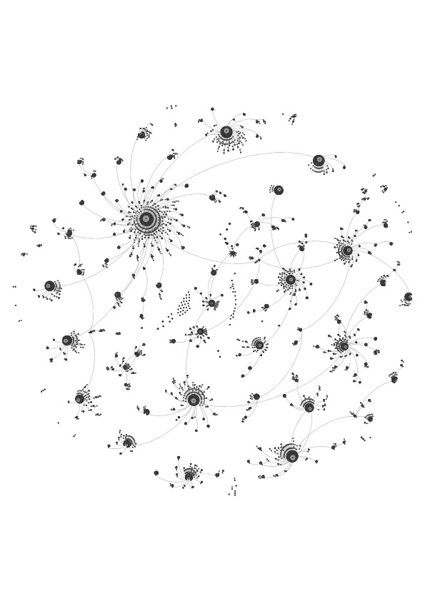
Figure 1. Visualization of Osama Bin Laden Diffusion. 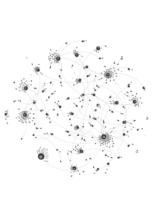
Figure 2. Visualization of Hurricane Irene Diffusion. 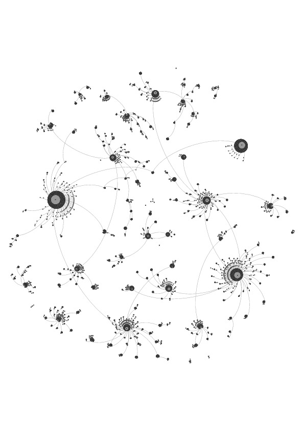
Figure 3. Visualization of Hurricane Sandy Diffusion. 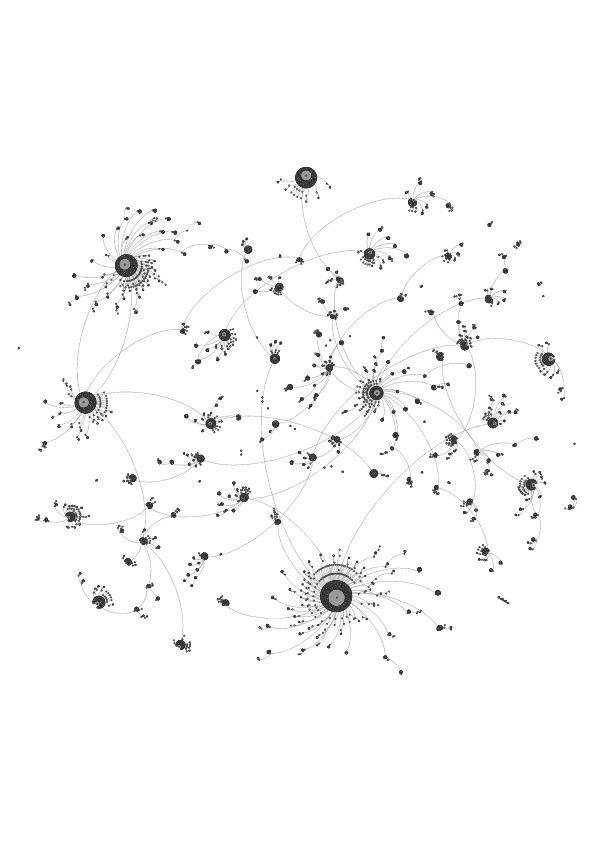
Figure 4. Visualization of US 2012 Presidential Election Diffusion. - 4.6
- Finally, we cleaned up the data to make it easily comparable to the model results. Using the same data that we used to create the graphs, we placed all of the data into bins of 1 hour intervals. That is, for each hour, we determined n(t), the number of people in the 15K network who sent their first tweet about the event during that hour. This allowed us to then build a standard adoption curve N(t), which is, for every hour of the dataset, the cumulative number of adopters (those who had tweeted about the event by that time). That is, N(t) = n(1) + ... + n(t).
Results
of the Comparison
- 5.1
- The next step was to compare the model to the data. Because
there was no obvious way to determine the values of the
 and
and  parameters that would achieve the best fit with the data, we conducted
a grid search to find the best parameter values. Initially we searched
the space coarsely at 0.01 increments, and then looked at a more
detailed level at 0.001 levels. Based on the initial search at 0.01
increments, we chose the space that appeared to minimize the error for
the finer grained search. In all of our investigations there appeared
to be one point that minimized the error
in the larger space and so we chose the same dimensions around that
point except where we encountered a boundary condition. For each model,
and
for each dataset we ran the model 10 times across this space. Each run
of
each model yielded values for Y(t),
the number of agents in the network
who had become aware at time t, and we calculated Z(t),
the average of the Y(t). The
standard deviations of these means were relatively low compared to the
means (averaging 0.04 of the mean across all data points, all networks
and all models, and never exceeding 0.19 of the mean for any
particular data series), and thus we feel 10 runs provides a decent
estimate of the
underling patterns (Details on all of this analysis is available from
the authors
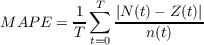
on request.). We then compared the simulated data Z(t)
to the real data, using Mean Absolute Percentage Error (MAPE), which is
the difference between
N(t), the actual value at
time t, and the average simulated value of time t,
divided by the actual value at time t (to transform
the absolute error into percentage error) and then averaged over all
points in
time:
parameters that would achieve the best fit with the data, we conducted
a grid search to find the best parameter values. Initially we searched
the space coarsely at 0.01 increments, and then looked at a more
detailed level at 0.001 levels. Based on the initial search at 0.01
increments, we chose the space that appeared to minimize the error for
the finer grained search. In all of our investigations there appeared
to be one point that minimized the error
in the larger space and so we chose the same dimensions around that
point except where we encountered a boundary condition. For each model,
and
for each dataset we ran the model 10 times across this space. Each run
of
each model yielded values for Y(t),
the number of agents in the network
who had become aware at time t, and we calculated Z(t),
the average of the Y(t). The
standard deviations of these means were relatively low compared to the
means (averaging 0.04 of the mean across all data points, all networks
and all models, and never exceeding 0.19 of the mean for any
particular data series), and thus we feel 10 runs provides a decent
estimate of the
underling patterns (Details on all of this analysis is available from
the authors
on request.). We then compared the simulated data Z(t)
to the real data, using Mean Absolute Percentage Error (MAPE), which is
the difference between
N(t), the actual value at
time t, and the average simulated value of time t,
divided by the actual value at time t (to transform
the absolute error into percentage error) and then averaged over all
points in
time:
(3) Table 1 gives the range that we investigated for each of the parameters, and the values (
 *,
*, *) which minimized
the average MAPE across all ten
runs.
*) which minimized
the average MAPE across all ten
runs.
Table 1: Range of parameter values and optimum values as determined by lowest MAPE. model dataset  range
range range
range

cascade bin laden 0.045 0.080 0.040 0.080 0.065 0.060 cascade irene 0.001 0.034 0.014 0.054 0.014 0.034 cascade sandy 0.001 0.027 0 0.020 0.007 0 cascade election 0.014 0.054 0 0.028 0.034 0.008 Bass bin laden 0.079 0.119 0 0.021 0.099 0.001 Bass irene 0.005 0.045 0 0.020 0.025 0 Bass sandy 0.001 0.024 0 0.029 0.004 0.009 Bass election 0.015 0.055 0 0.023 0.035 0.003 - 5.2
- The comparison between the underlying data and the model
results is visible in the following graphs. Figures 5
and 6 illustrate the two fits
to the Bin Laden data. Figures 7
and 8 illustrate the two fits
to the Hurricane Irene data. Figures 9
and 10 illustrate the two fits
to the Hurricane Sandy data. Figures 11
and 12 illustrate the two fits
to the US 2012 Presidential Election
data. As can be seen most of the data follows a fairly monotonic and
increasing
path. However, the Bin Laden, in particular, features multiple
acceleration in the influx of data. In this case, the news was released
late at night, and some individuals did not respond to the next
morning. So the double hump is present due to some users tweeting at
the time of release and others tweeting when they awoke the next day.
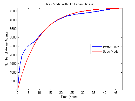
Figure 5. Comparison of best matching Bass model to Bin Laden data. 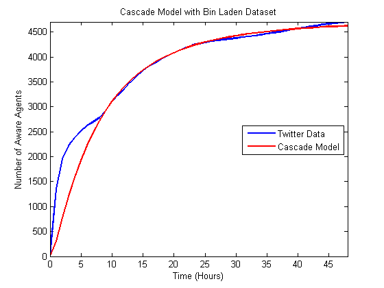
Figure 6. Comparison of best matching independent cascade model to Bin Laden data. 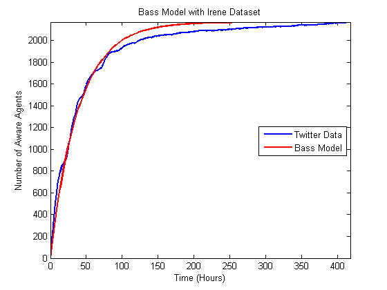
Figure 7. Comparison of best matching Bass model to the Hurricane Irene data. 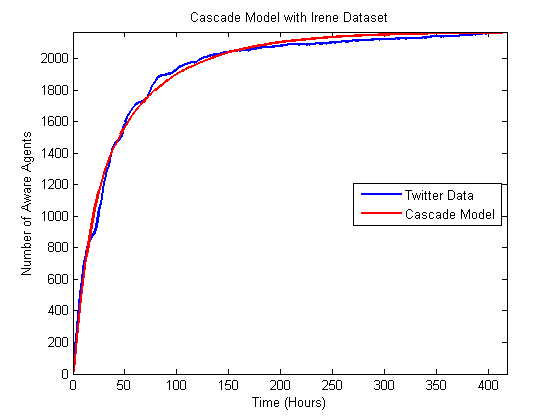
Figure 8. Comparison of best matching independent cascade model to the Hurricane Irene data. 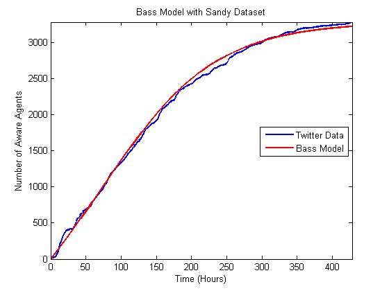
Figure 9. Comparison of best matching Bass model to the Hurricane Sandy data. 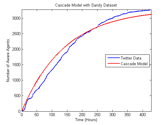
Figure 10. Comparison of best matching independent cascade model to the Hurricane Sandy data. 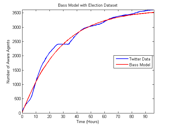
Figure 11. Comparison of best matching Bass model to the Election data. 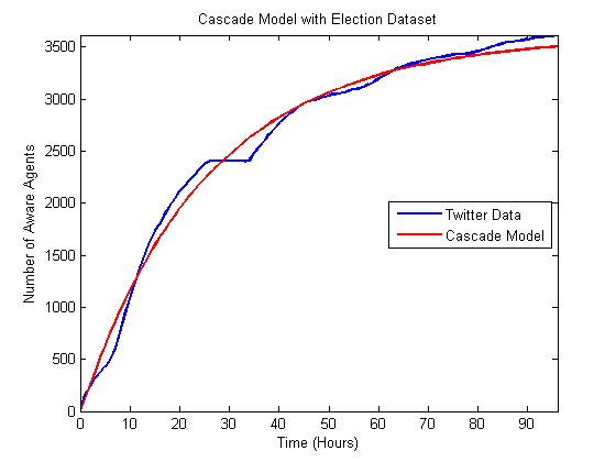
Figure 12. Comparison of best matching independent cascade model to the Election data. - 5.3
- To further explore the sensitivity of the model to the
parameters that we were exploring, we also explored the full MAPE
values for all of the
 and
and  values around
the identified optimal values. Heatmaps of these results are presented
in the following figures. Figures 13
and 14 illustrate sensitivity
of the Bin Laden data. Figures 15
and 16 illustrate the
sensitivity of the Hurricane Irene data. Figures 17
and 18 illustrate the
sensitivity of the Hurricane Sandy data. Figures 19
and 20 illustrate the two fits
to the US 2012 Presidential Election data. In these heat
maps, lower values are darker blues, and higher values are brighter
reds,
so areas of dark blue indicate areas with minimal errors and, thus,
closest
fits. As is illustrated in these figures for all datasets and all
models the data trends toward one particular point indicating that at
least for the spaces explored the error in the model is unimodal, i.e.,
there is one optimal set of parameters that minimizes the error.
values around
the identified optimal values. Heatmaps of these results are presented
in the following figures. Figures 13
and 14 illustrate sensitivity
of the Bin Laden data. Figures 15
and 16 illustrate the
sensitivity of the Hurricane Irene data. Figures 17
and 18 illustrate the
sensitivity of the Hurricane Sandy data. Figures 19
and 20 illustrate the two fits
to the US 2012 Presidential Election data. In these heat
maps, lower values are darker blues, and higher values are brighter
reds,
so areas of dark blue indicate areas with minimal errors and, thus,
closest
fits. As is illustrated in these figures for all datasets and all
models the data trends toward one particular point indicating that at
least for the spaces explored the error in the model is unimodal, i.e.,
there is one optimal set of parameters that minimizes the error.
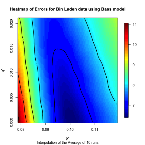
Figure 13. Heat map illustrating the sensitivity of the Bass model on the Bin Laden data. 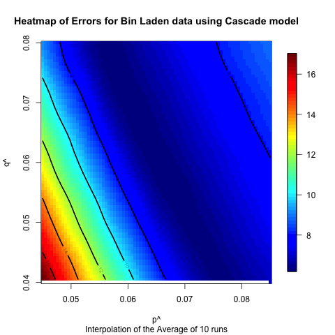
Figure 14. Heat map illustrating the sensitivity of the independent cascade model on the Bin Laden data. 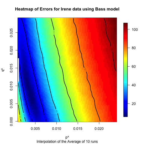
Figure 15. Heat map illustrating the sensitivity of the Bass model on the Hurricane Irene data. 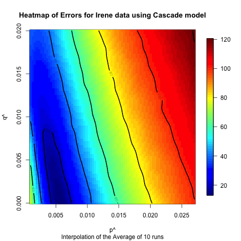
Figure 16. Heat map illustrating the sensitivity of the independent cascade model on the Hurricane Irene data. 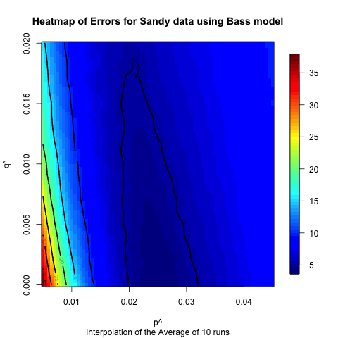
Figure 17. Heat map illustrating the sensitivity of the Bass model on the Hurricane Sandy data. 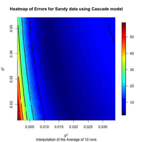
Figure 18. Heat map illustrating the sensitivity of the independent cascade model on the Hurricane Sandy data. 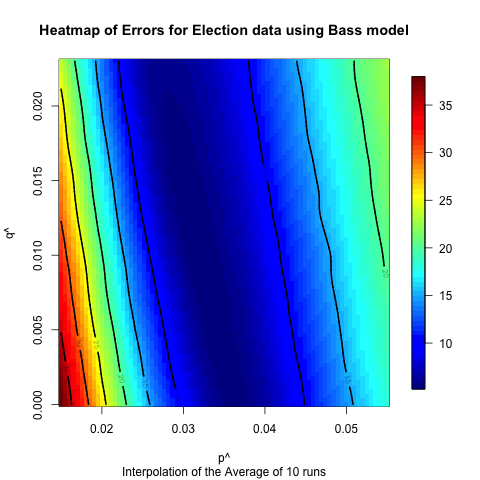
Figure 19. Heat map illustrating the sensitivity of the Bass model on the Election data. 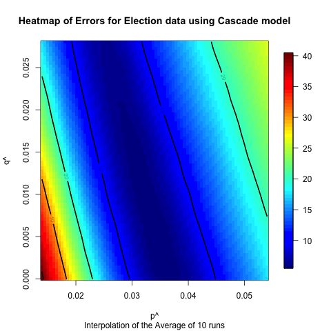
Figure 20. Heat map illustrating the sensitivity of the independent cascade model on the Election data.
Discussion
and Future Work
- 6.1
- Based on the comparison between the model and real data, it appears that the models can fit the data better for the hurricane cases, which have longer time horizons and, we hypothesize, numerous subevents. In some ways these events are closer to the type of diffusion events for which these models were originally created. The Bin Laden and Election cases have shorter time horizons, and the models do not fit as well. However, despite the fact that these models were not originally created to examine the diffusion of urgent information, they fit fairly well based on observed differences between the model output and the actual data. Moreover, the heat maps illustrate that these results are fairly robust to changes in the underlying parameters. In many of the cases altering the input parameters by half an order of magnitude will still only mean that the prediction is off by less than 10 to 20%. Of course, it would be easy to create polynomial regression that would fit this data also, but since we are building the model at the level of the individuals, we can proceed to asking how various policies would alter the diffusion of information. For instance, if a nongovernmental organization wanted to spread a particular message about an upcoming urgent event, they could explore who should be contacted to spread that message.
- 6.2
- The heat maps also indicate that for most of the models and datasets that we examined there is a range of values that produce similar results. This seems to indicate that though we have identified “robust” values for each of the network and model combinations, there is a range of values for which the match will be fairly good. This indicates that one does not have to have the values exactly right for the models to have decent predictive value. Moreover, the differences between the Bass and independent cascade models, both in terms of the robustness of the results and the best fits, were not very significant, which indicates that of these two models there is not a clear “best” model, so either is appropriate for future exploration. However, it does appear that the event has a large impact on the fit of the results, which seems to indicate that having the ability to classify events ahead of time in order to identify appropriate ranges of these values is useful, and we will explore this in future work.
- 6.3
- We hypothesize that we can improve these models in a number of different ways to improve their accuracy. The basic Bass model and the independent cascade model were originally created for longer time frames, and urgent diffusion events happen on a much faster pace, especially given the current 24-hour news cycle. In previous work, we constructed a purely statistical, stochastic model (with no network information) that includes the diurnal cycle of Twitter activity, which can achieve a better fit to the data than the models used in this scenario. This is clearly illustrated in the Osama bin Laden case, where the diurnal cycle is readily apparent in Figures 5 and 6. Thus, it would be useful to include agent behaviors that reflect this diurnal cycle. In addition, new information about an event begins spreading while the first information continues to spread. If we can model the entrance of this external information, we could also improve the model. We have previously done this in the math-based model, by simply estimating a daily “shock” to the system, and this method could easily be adapted to the agent-based model, though it would introduce a number of new parameters to the system. In future work, we hope to tie the external shocks directly to another data source such as stories in mainstream media. We will also compare the spread of information across populations that are connected via social media to the spread of information across populations that are not connected to determine when and how much the social media connections accelerate information diffusion.
- 6.4
- The overall goal for this project is to provide recommendations for policy makers, brand managers, and other interested parties about how information will diffuse in urgent situations. Eventually, we would like to make these models predictive, by providing a set of guidelines for how to run a model for an event that is in the process of occurring, by tying the type of event to the parameter space. For instance, it is possible that hurricanes always generate “Type 1” events that are different than major news stories, such as the Bin Laden or Election data, which could be called “Type 2” events. This would then provide interested stakeholders with a set of parameters to feed into the system, giving them the ability to predict how fast and to whom information would diffuse. This, in turn, would allow them to make decisions about how to reach out with accurate information and predict how quickly a population will react to that information.
Acknowledgements
-
We would like to thank the anonymous reviewers from the CSSSA meeting where this paper was originally presented, as well as the feedback from the participants of that meeting. We would also like to thank the anonymous reviewer who provided us with comments while reviewing for JASSS.
Notes
-
1An
earlier version of this paper was presented at the Computational Social
Science Society.
2Since
 and
and  are not equivalent to the hazard rates, p and q,
above, we use the “hat” notation to separate them.
are not equivalent to the hazard rates, p and q,
above, we use the “hat” notation to separate them.3Though clearly the exact values of the independent cascade model
 and
and  will differ from those used in the Bass model, their meaning is very
similar. For the sake of brevity we use the same notation for both
models.
will differ from those used in the Bass model, their meaning is very
similar. For the sake of brevity we use the same notation for both
models.
Appendix
-
In this section, we will describe the model in more detail, using a description based on ODD (Overview, Design concepts, Details) protocol for describing individual- and agent-based models (Grimm et al. 2010).
Purpose
The purpose of this model is to better understand the diffusion of information in urgent situations. The model is intended to be used by any number of stakeholders to understand how a particularly urgent topic might diffuse through a large group of individuals on social media. With this understanding, users might be able to better engage with social media, and better understand real-world reactions to conversations on social media. Though the current model only explores how well the model fits available data, in future work we plan to explore optimal policies for social media engagement.
Entities, state variables, and scales
One basic entity in the model is a user of social media who is interesting in consuming and transmitting information. All told these entities exist within the general scope of a social network, via a social media platform. In this paper, we examined individuals involved in Twitter conversations. As a result, another basic entity of the model is the link or relationship between two individuals. These links mean that one user is connected to another user in a way that enables the transmission of information. In the case of Twitter, we use the following relationship as indication of a social connection.
The social media user agents in the model have a number of different state variables. First, they have a property which specifies whether or not they have adopted the new piece of information. In addition, they have both a
 ,which is the coefficient of innovation, and
  which is the coefficient of imitation. These determine how individuals
make a decision to adopt or not adopt a new piece of information. All
agents in the model also possess a
set of links which are the social relationships of that user to other
users. In
the current version of the model, the links themselves have no
properties,
but are directed links indicating that one user ”follows“ another user
on
Twitter.
which is the coefficient of imitation. These determine how individuals
make a decision to adopt or not adopt a new piece of information. All
agents in the model also possess a
set of links which are the social relationships of that user to other
users. In
the current version of the model, the links themselves have no
properties,
but are directed links indicating that one user ”follows“ another user
on
Twitter.
As to the scales of the properties and entities, there is a one-to-one mapping between social media user agents and real Twitter users as identified by our 15K collection. This collection is a snowball network sample of 15,000 active, non-celebrity users, including all of the connections between those users. In order to contain noise, we focused on active users that were discovered during our snowball sample. Active users that form part of our dataset issued an average one tweet per day in latest 100 tweets, and had at least one retweet in the latest 100 tweets. Also with respect to scale, the
 and
and  properties can be considered
to be probabilities of an event occurring. Finally, the time step of
this model is one hour. All simulations were run for the length of time
that it took to match the underlying data.
properties can be considered
to be probabilities of an event occurring. Finally, the time step of
this model is one hour. All simulations were run for the length of time
that it took to match the underlying data.
Process overview and scheduling
The underlying process model is fairly simple. The basic idea is that all agents are initialized to an unadopted state, and at the same time the social network between the agents is constructed. Then at each time step any agents which still have not adopted the new information, determine (probabilistically) if they should adopt the new information based on
 and
and  and the state of their neighbors. This basic overview is true
regardless of which model of adoption (Bass or independent cascade) is being used;
the only thing that changes is the decision
rule.
and the state of their neighbors. This basic overview is true
regardless of which model of adoption (Bass or independent cascade) is being used;
the only thing that changes is the decision
rule.
The submodels will be discussed below but the basic processes are:
- Initialize Network and Agents
- Repeat for Number of Hours in Event
a. For each Social Media User Agent that has not adopted:
i. Decide to Adopt based on and
and 
ii. Update State of Agent based on Decision
b. Update Statistics
Design Concepts
In this section we will explore the design concepts of the model.
Basic Principles
The key aspect of this model that is emergent is the overall adoption rate of the new information. This is modeled by assuming that a small percentage of the population finds out about the new information every time step and that they spread that information via their social networks.Adaptation
Agents in the model are not really adaptive since they do not change as a result of their past experience. Instead they simply react to the presence of information among their neighbors and then decide whether or not to adopt the information.
Objectives
The agents do not have particular objectives, but instead simply make decisions about whether or not to adopt novel information.
Learning
The agents in the model do not learn.
Prediction
Agents do not make any predictions about future states of the world.
Sensing
The social media user agents can sense the state of their immediate neighbors that they are following. For instance, they know what fraction of their neighbors have adopted the information, and whether or not it was adopted in the previous time step.
 can also be thought of as the sensing of an external source of
information that
informs the agent about the new information.
can also be thought of as the sensing of an external source of
information that
informs the agent about the new information. Interaction
The social media user agents interact with each other by exchanging new information. Each agents determines whether or not to adopt the new information based on the submodels described below.
Stochasticity
At each time step of the model, each agent who has not adopted the information draws random numbers on the uniform interval [0,1] to determine if they should adopt the information or not. These random numbers are compared to both
 and
and  to determine if they should
adopt the information or not.
Because of this each run of the model can result in very different
diffusion
patterns.
to determine if they should
adopt the information or not.
Because of this each run of the model can result in very different
diffusion
patterns. Collectives
There is one major collective in the model, which is the social network connecting all of the users. Of course, in the standard social network sense, cliques also exist within the networks which can be thought of as smaller collectives.
Observation
For the purposes of this paper, the observation we are most concerned with is the overall adoption of the information at each time step of the model run. We are then comparing this information to empirical data to determine which values of
 and
and  best match the observed empirical data.
Initialization
The following steps are the major parts of the initialization:
- Create a number of social media user agents equivalent to the final number that tweet in this dataset
- Initialize all of the social media user agents to the unadopted state
- Set the
 and
and  of all agents to the values
currently being explored
of all agents to the values
currently being explored
- Connect the social media agents together using the social network data from the 15K network
Input Data
The only major source of input data is the 15K network data about who is collected to whom in Twitter, based on the snowball sample described in Entities section of the ODD protocol. However, there were also four datasets collected from Twitter by filtering out tweets that matched certain keywords. These datasets were used to establish the validity and examine differences in the underlying model:
- Bin Laden - this dataset examines the 48 hours after Osama Bin Laden’s capture and death, and contain all of the tweets that had the words related to this event in them. The dataset contains 13,842 edges, which come from an initial 1231 tweeters
- Irene - This dataset examines roughly a week around the landfall and aftermath of Hurricane Irene. This dataset contains 14,373 edges, which come from an initial 814 tweeters.
- Sandy - This dataset examines roughly a week around the landfall and aftermath of Hurricane Sandy. The dataset contains 14,508 edges, which come from an initial 839 tweeters.
- Election - This dataset examines the 25 hour period from midnight the night before the US 2012 Presidential National election to 1 AM the next morning. The election dataset contains 13,408 edges, which come from an initial 832 tweeters.
Since these datasets describe the total space of people who discussed these topics within the 15K dataset they were used to determine how many agents would be created in each model.
Submodels
There are two major submodels that are involved in the decision of users to adopt: (1) the Bass model, and (2) the independent cascade model.
Bass Model
Based on a hazard-rate model that was originally developed to understand the adoption of consumer durables (Bass 1969), the agent-based Bass model is a discrete-time model in which each agent has one of two states at each time step t: (1) unaware or (2) aware. At the beginning of the simulation, all agents are unaware. At each time step, an unaware agent has an opportunity to become aware. Its state changes with a probability that reflects advertising and word-of-mouth effects. The probability that an agent becomes aware due to word of mouth increases as a function of the fraction of its neighbors who became aware in previous time steps. Once an agent becomes aware, it remains aware for the rest of the simulation.
At each time step, an unaware agent i becomes aware due to one of two circumstances:
- Innovation - With probability
 ,
an unaware agent becomes aware due to outside effects, i.e.,
information from outside the network, where
,
an unaware agent becomes aware due to outside effects, i.e.,
information from outside the network, where  is
the coefficient of innovation.
is
the coefficient of innovation.
- Imitation - With probability f
 ,
an unaware agent becomes aware due to observing the awareness of its
neighbors, where f is the fraction of neighbors who
have adopted and
,
an unaware agent becomes aware due to observing the awareness of its
neighbors, where f is the fraction of neighbors who
have adopted and  is the coefficient of imitation.
Independent Cascade Model
The second diffusion model that we examined was the independent cascade Model (Goldenberg et al. 2001). The basic idea behind the independent cascade model is that an individual has probability
 of becoming aware at any time step when m
of their neighbors have become aware. There is also a small a
probability
of becoming aware at any time step when m
of their neighbors have become aware. There is also a small a
probability  that the individual becomes aware due to
advertising or external news events. The basic intuition behind the
independent cascade model is that information and adoption decisions ripple through
a social network in cascades, rather than in long-term exposures such
as the Bass model denotes.
that the individual becomes aware due to
advertising or external news events. The basic intuition behind the
independent cascade model is that information and adoption decisions ripple through
a social network in cascades, rather than in long-term exposures such
as the Bass model denotes.
For the agent-based model, a population of agents on a network is created, and all of the agents are initially unaware then at each time step each agent becomes aware due to two circumstances that are similar to the Bass rules:
- Innovation - With probability
 , an unaware agent
becomes aware due to outside effects, i.e., information from outside
the network, where
, an unaware agent
becomes aware due to outside effects, i.e., information from outside
the network, where  is the coefficient of innovation.
- Imitation - With probability
 ,
an unaware agent becomes aware if any of its neighbors have adopted in
the previous time step and
,
an unaware agent becomes aware if any of its neighbors have adopted in
the previous time step and  is the coefficient of imitation.
References
- ABBASI, M.-A., Kumar, S., Filho,
J. A. A., & Liu, H. (2012, January). Lessons learned in using
social media for disaster relief - ASU crisis response game. In S. J.
Yang, A. M. Greenberg, & M. Endsley (Eds.), Social
computing, behavioral - cultural modeling and prediction
(pp. 282–289). Springer Berlin Heidelberg.
BASS, F. M. (1969, January). A new product growth for model consumer durables. Management Science, 15(5), 215–227. Available from <http://mansci.journal.informs.org/content/15/5/215>
BASTIAN, M., Heymann, S., & Jacomy, M. (2009). Gephi: an open source software for exploring and manipulating networks. In Icwsm.
BORGE-HOLTHOEFER, J., Baños, R. A., González-Bailón, S., & Moreno, Y. (2013). Cascading behaviour in complex socio-technical networks. Journal of Complex Networks, 1(1), 3–24. [doi:10.1093/comnet/cnt006]
GOLDENBERG J., Libai B., & Muller E. (2001). Talk of the network: A complex systems look at the underlying process of word-of-mouth. Marketing Letters, 12(3), 211–223. [doi:10.1023/A:1011122126881]
GRANOVETTER, M. (1978). Threshold models of collective behavior. American journal of sociology, 1420–1443. [doi:10.1086/226707]
GRIMM, V., Berger, U., DeAngelis, D. L., Polhill, J. G., Giske, J., & Railsback, S. F. (2010). The odd protocol: a review and first update. Ecological Modelling, 221(23), 2760–2768. [doi:10.1016/j.ecolmodel.2010.08.019]
HUGHES, A. L., & Palen, L. (2009). Twitter adoption and use in mass convergence and emergency events. International Journal of Emergency Management, 6(3), 248–260. [doi:10.1504/IJEM.2009.031564]
LERMAN, K., & Ghosh, R. (2010). Information contagion: An empirical study of the spread of news on digg and twitter social networks. In International conference on weblogs and social media.
NEKOVEE, M., Moreno, Y., Bianconi, G., & Marsili, M. (2007). Theory of rumour spreading in complex social networks. Physica A: Statistical Mechanics and its Applications, 374(1), 457–470. [doi:10.1016/j.physa.2006.07.017]
PALEN, L., Anderson, K. M., Mark, G., Martin, J., Sicker, D., Palmer, M., et al. (2010). A vision for technology-mediated support for public participation & assistance in mass emergencies & disasters. In Proceedings of the 2010 acm-bcs visions of computer science conference (p. 8).
RAND, W., & Rust, R. T. (2011). Agent-based modeling in marketing: Guidelines for rigor. International Journal of Research in Marketing, 28(3), 181–193. [doi:10.1016/j.ijresmar.2011.04.002]
ROGERS, E. M. (2010). Diffusion of innovations. Simon and Schuster.
SHKLOVSKI, I., Palen, L., & Sutton, J. (2008a). Finding community through information and communication technology in disaster response. In Proceedings of the 2008 ACM conference on computer supported cooperative work (p. 127136). New York, NY, USA: ACM. Available from <http://doi.acm.org/10.1145/1460563.1460584>
SHKLOVSKI, I., Palen, L., & Sutton, J. (2008b). Finding community through information and communication technology in disaster response. In Proceedings of the 2008 acm conference on computer supported cooperative work (pp. 127–136).
SUTTON, J., Palen, L., & Shklovski, I. (2008). Backchannels on the front lines: Emergent uses of social media in the 2007 southern california wildfires. Proceedings of the 5th International ISCRAM Conference, 624–632.
TRUSOV, Michael, Rand, W., & Joshi, Yogesh. (2013). Product diffusion and synthetic networks: Improving pre-launch forecasts with simulated priors. Working Paper.
VALENTE, T. W. (1995). Network models of the diffusion of innovations (quantitative methods in communication series). Hampton Press (NJ) (January 10, 1995).
VERMA, S., Vieweg, S., Corvey, W. J., Palen, L., Martin, J. H., Palmer, M., et al. (2011a). Natural language processing to the rescue?: Extracting'Situational awareness' tweets during mass emergency. Proc. ICWSM.
VERMA, S., Vieweg, S., Corvey, W. J., Palen, L., Martin, J. H., Palmer, M., et al. (2011b). Natural language processing to the rescue? extracting" situational awareness" tweets during mass emergency. In Icwsm.
VIEWEG, S., Hughes, A. L., Starbird, K., & Palen, L. (2010). Microblogging during two natural hazards events: what twitter may contribute to situational awareness. In Proceedings of the sigchi conference on human factors in computing systems (pp. 1079–1088). [doi:10.1145/1753326.1753486]
WATTS, D. J. (2002). A simple model of global cascades on random networks. Proceedings of the National Academy of Sciences, 99(9), 5766–5771. [doi:10.1073/pnas.082090499]
YIN, J., Lampert, A., Cameron, M., Robinson, B., & Power, R. (2012). Using social media to enhance emergency situation awareness. IEEE Intelligent Systems, 27(6), 52–59. [doi:10.1109/MIS.2012.6]
ZHANG, Z.-l., & Zhang, Z.-q. (2009). An interplay model for rumour spreading and emergency development. Physica A: Statistical Mechanics and its Applications, 388(19), 4159–4166. [doi:10.1016/j.physa.2009.06.020]
ZHAO, L., Wang, J., Chen, Y., Wang, Q., Cheng, J., & Cui, H. (2012). Sihr rumor spreading model in social networks. Physica A: Statistical Mechanics and its Applications, 391(7), 2444–2453. [doi:10.1016/j.physa.2011.12.008]
ZHAO, L., Wang, Q., Cheng, J., Chen, Y., Wang, J., & Huang, W. (2011). Rumor spreading model with consideration of forgetting mechanism: A case of online blogging livejournal. Physica A: Statistical Mechanics and its Applications, 390(13), 2619–2625. [doi:10.1016/j.physa.2011.03.010]