
 Abstract
- The availability of refuelling locations for alternative fuel vehicles (AFVs) is an important factor that drivers consider before adopting an AFV; thus, the layout of initial filling stations for AFVs will influence the adoption of AFVs. This paper presents a training system for optimising the layout of initial filling stations for AFVs by linking an agent-based model of the adoption of AFVs with a real city/area's road network, as well as the city/area's social and economic background. In the agent-based model, two types of agents (driver agents and station owner agents) interact with each other in a city/area's road network, stored in a GIS (Geographic Information System). With simulation scenario analyses and a genetic algorithm, the training system presented in this paper can help decision makers determine close-to-optimal layouts for initial AFV filling stations. This paper also presents a case study of the application of the training system that analyses the layout of fast-charging or battery-changing stations for the promotion of electric vehicles adoption in Shanghai.
- Keywords:
- Training System, Optimal Layout, Alternative Fuel Vehicles, Filling Stations
Introduction
- 1.1
- With increasing concerns regarding climate change and the depletion of fossil fuels, developing alternative fuel vehicles (AFVs) has become a national technology strategy for many countries, e.g. (China's State Council 2012; US Department of Energy 2013). AFVs, such as fuel cell-powered vehicles, are currently more expensive than traditional gasoline-powered vehicles. It is widely believed that technological learning, i.e. the cost of using a new technology tends to decrease as experience in it accumulates (Arrow 1962), will be an endogenous driving force for the adoption of AFVs (Schwoon 2008). However, there is a "chicken or egg" dilemma between AFVs and their corresponding filling stations: drivers are reluctant to switch to AFVs if they find that compatible filling stations are rare, and energy providers are reluctant to build filling stations for AFVs if they find that few people are using them. With the "chicken or egg" dilemma, it is difficult for technological learning to take off. To promote the adoption of AFVs, governments must organise some initial filling stations as the "seeds" for technological learning. Where should these initial filling stations be located so that they can induce a successful diffusion of AFVs? It is difficult to answer this question with traditional operational approaches and equilibrium analysis because the adoption of AFVs is a complex process that involves various heterogeneous actors interacting with each other. The main research contribution of this study is a methodology to help decision makers find an appropriate layout of initial filling stations by linking an agent-based model with real social-economic data and a real road network in a GIS (Geographic Information System). Here, the decision makers could be government officials or a company's managers. When a project for establishing initial filling stations for AFVs is initialised and massively sponsored by governments, the decision makers are government officials. It is also possible that a leading company could set initial filling stations for its own business; for example, Tesla has started constructing initial recharging stations for its electric vehicles in the US[1]. In this case, the decision makers are the company's managers.
- 1.2
- Agent-based models (ABMs) are considered to be powerful tools for studying complex systems involving heterogeneous actors (Arthur 1999; Farmer & Foley 2009). Agents in ABM are defined as autonomous decision-making entities. From the standpoint of artificial intelligence, an agent is a computer system that is either conceptualised or implemented using concepts that are more typically applied to humans (Wooldridge & Jennings 1995). ABMs have been applied to address dynamics resulting from interactions among heterogeneous actors in various fields, such as stock markets (e.g., Palmer et al. 1994), dissemination of culture, e.g. (Axelrod 1997), electricity trading, e.g. (Bunn & Oliveira 2001), co-evolution of parochial altruism and war, e.g. (Choi & Bowles 2007), evacuations from buildings that are on fire, e.g. (Shi et al. 2009), the spread of contagious diseases, e.g. (Beyrer et al. 2012) or technologies, e.g. (Delre et al. 2007), and many others. Agent-based modelling and simulation has also been used for decision support, e.g. (Strader et al. 1998; Lee & Lee 2007).
- 1.3
- Stephan and Sullivan (2004) put forward a stylised ABM to simulate the co-adoption of fuel cell vehicles and hydrogen filling stations in an urban area. In their model (henceforth the SS model), they define two types of agents: driver agents and station owner agents. The co-adoption of fuel cell vehicles and hydrogen filling stations is the result of the interactions among the agents in an urban area, which was denoted by a square space with intersecting roads forming right angles. Their stylised model and simulations can help people to understand the complexity of the adoption process of AFVs, but their work did not incorporate a real city/area's social and economic background. Thus, it cannot provide decision support for a specific city/area to solve the problem of designing a close-to-optimal layout of initial filling stations for AFVs.
- 1.4
- In this paper, we develop a training system by linking a SS-like agent-based model of AFV adoption with a real city/area's road network, as well as the city/area's social and economic background, in a Geographic Information System (GIS). The system can aid decision makers' intuition in finding a close-to-optimal layout of initial filling stations via simulation scenario analysis and a genetic algorithm.
- 1.5
- Our study is limited to AFVs that have a similar refuelling pattern to that of traditional vehicles, i.e., these vehicles must go to a refuelling/recharging station, and the refuelling or recharging routinely takes several minutes. Recently, electric vehicles have appeared as promising AFVs, e.g. (US Department of Energy 2013). Quickly recharging depleted batteries or using robots to exchange them with fully charged ones, which would only take several minutes, present a promising system for electric vehicles. The AFVs in this paper are modelled as these types of electric vehicles, and the filling stations presented are considered either fast-charging or battery-changing stations. The framework of the model and the training system presented in this paper also apply to other AFVs, such as hydrogen fuel cell vehicles or gas-fueled vehicles, but it does not apply to electric vehicles that need several hours for recharging[2]. With the aim of providing a general training system for the initial layout of any type of AFV with refuelling/recharging patterns similar to those of traditional vehicles, this paper does not go into the details of the technological or economic features of different AFVs. As a case study of the application of the training system, this paper presents an analysis of the initial layout of fast-charging or battery-changing stations for promoting the adoption of electric vehicles in Shanghai.
- 1.6
- The remainder of this paper is organised in the following manner. Section 2 provides the framework of the training system. Section 3 introduces the SS-like agent-based mode and its linkage with GIS and a real city/area's social and economic background. Section 4 presents the method of getting a close-to-optimal layout of initial filling stations. Section 5 provides a case study of the application of the training system. Section 6 presents the concluding remarks.
The framework of the training system
- 2.1
- Figure 1 illustrates the framework of the training system, which can be divided into three parts represented in white and two shades of grey. The first part is the core, the model of the training system, which is in the middle of Figure 1. In this part, the stylised space in an SS-like agent-based model is replaced with a specific city/area's road network in a GIS, and the driver agents' driving routes are generated from the social and economic data of the specific city/area. The second part is the data on the AFVs' technological and economic features, the road network, and the social and economic data of the specific city/area. Such data commonly need be specified by researchers. The third part is the input and output interface for the users (the decision makers or their assistants). With the third part, users can set different layouts of the initial filling stations, either with a graphical user interface (GUI) or with a genetic algorithm (GA). Given different initial layouts, simulations with the ABM will generate different adoption scenarios of the AFVs, and the decision makers can select the layout that generates the fastest adoption scenarios as the close-to-optimal solution. At the early stages of AFV adoption, governments may establish a policy of subsidising the AFVs. Thus, in the third part, the system also incorporates public policy by allowing users to set the intensity of a government's AFV subsidy.
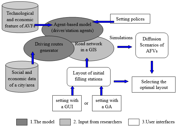
Figure 1. The framework of the training system - 2.2
- Figure 2 shows the main GUI interface of the training system. Window A in Figure 2 is the window for setting the number of initial filling stations. After setting the number of initial filling stations, users can either set their locations one-by-one, manually, with window B by pushing the Manual button, or set them with the GA-based method, which will be introduced in section 4, by pushing the GA button. Window C is for setting parameters, such as the number of driver agents, the government's subsidy, and so on. Window D is for controlling the starting, pausing and ending of the simulation. Window E shows the dynamics of the number of AFV adopters. Window F shows the dynamics of the number of filling stations of AFVs. Window G shows the dynamics of distributions of filling stations. Window H is for selecting and editing different road maps.
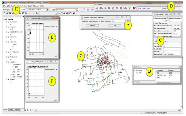
Figure 2. The main GUI interface of the training system
The model
- 3.1
- We describe the model following the ODD (Overview, Design concepts and Details) protocol (Grimm et al. 2006).
Purpose
- 3.2
- The purpose of the model is to simulate the co-diffusion of AFVs and their filling stations in an urban city with different layouts of initial filling stations and the training system developed based on the model aims to help decision makers to find a close-to-optimal layout of initial filling stations via simulation scenario analysis and a genetic algorithm.
State variables and scales
- 3.3
- There are two types of agents in the model: driver agents and station owner agents. Driver agents are characterised by the state variables: identity number, living location, working location, time period of buying a new vehicle. Driver agents will calculate their concerns on refuelling an AFV with the availability of filling stations in its driving paths, and also the utility of using an AFV. We use several thousand, e.g. (8000 in the case study presented in section 5) driver agents to represent the drivers in an urban city. Station owner agents are characterised by the state variables: identity number, location, and threshold for surviving. Each station owner agent operates one filling stations for AFVs. We assume there are several, e.g. (10 in the case study presented in section 5) initial filling stations (owner agents) for AFVs. During the simulation, new filling stations (owner agents) will come into being and some existing ones will disappear.
- 3.4
- In addition to driver agents and station owner agents, other entities in the model are AFVs, a government, and an urban city. All AFVs are homogenous with a technological learning rate. The government gives a subsidy to driver agents who buy AFVs. The urban city is composed of several districts, e.g., 19 districts in Shanghai, including both the centre and suburbs of the city. The road network in our simulations includes main roads in the urban city.
- 3.5
- One step in the simulation represent one month, we run each simulation for 180 months (15 years).
Process overview and scheduling
- 3.6
- With each step (or month), four modules or phases are processed in the following order.
1. Switching to AFVs. This phase includes the following three sub-phases.- Buying or not. Each driver agent checks whether it is time to buy a new vehicle, the buying decision following a lognormal distribution.
- Calculating utility. Each driver agent who will buy a new vehicle calculates the utility of using an AFV.
- Selecting a vehicle. Each driver agent who will buy a new vehicle with a positive utility of using an AFV selects an AFV, otherwise it selects a traditional vehicle.
3. Coming of new station owner agents. New station owner agents appear in the places where there are enough AFVs passing through these places.
4. Updating AFVs' cost. The new cost of AFVs is calculated with technological learning effect.Design concepts
- 3.7
- Emergence: The diffusion of AFVs emerges from each driver agent's decision of adopting an AFV based on its utility of using an AFV. The diffusion of filling stations emerges from station owners decisions on establishing new or closing existing filling stations.
- 3.8
- Adaption: Driver agents will switch to AFVs or traditional vehicles based on their utilities of using AFVs. Station owner agents will open or close AFVs' filling stations based on their observations on the number of potential customers.
- 3.9
- Sensing: Driver agents know the locations of filling stations in their driving paths and based on which they have different concerns on availability of refuelling AFVs. Station owner agents know the number of AFVs passing through their locations and they also know the threshold number for their surviving.
- 3.10
- Interaction: The number and layout of station owner agents (i.e., filling stations) will influence driver agents' concern on availability of refuelling AFVs. And in turn, the number of driver agents adopting AFVs will influence the coming of new station owner agents and surviving of existing station owner agents. The number of driver agents adopting AFVs will influence AFVs' technological learning effect, and in turn technological learning effect will influence the cost of AFVS and thus influence the number of driver agents adopting AFVs.
- 3.11
- Stochasticity: Driver agents' intervals of buying a new vehicle follow a normal distribution.
- 3.12
- Observation: The number of driver agents adopting AFVs and the number of filling stations are recorded step by step. The dynamics (coming, existing, and disappearing) of station owner agents is displayed in a GIS map step by step.
Initialisation
- 3.13
- In the case study presented in section 5, the simulations start with 8000 driver agents, 0.05% of them are assumed to have adopted AFVs. The living and working places are initialised based on the spatial distribution of population and GDP in Shanghai. There are 10 initial filling stations for AFVs. In different simulations, the layout of initial filling stations could be initialised different (for studying what type of layout is better for the diffusion of AFVs). The initial cost of AFVs is set based on the evaluation on the average cost of AFVs. The road network includes the main roads in Shanghai. Driver agents' living and working places are determined following the spatial distribution of Shanghai's population and GDP (Gross Domestic Production). Driver agents' driving routes to attractions, e.g. (Shopping malls) are generated randomly following a Poisson distribution.
Input
In the current model, with initialisation, the simulation process is not affected by external (or environmental) dynamics. In the future, we would consider including external dynamics in price of gasoline, number of driver agents, and so on.Submodels
-
Driver agents
- 3.14
- A driver agent will update his/her vehicle after a certain number of years, which exhibit a normal distribution. When updating his/her vehicle, a driver agent will evaluate the utility of using an AFV, as shown in Eq. (1).
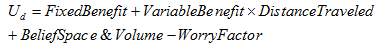
(1) where Ud represents a driver agent's utility of using an AFV. FixedBenefit represents the benefit of the lower cost of buying an AFV with a government subsidy. Because an AFV is usually more expensive than a traditional vehicle, the FixedBenefit variable can be negative. With more drivers switching to the AFVs, their cost could decrease as a result of the technological learning effect (Arrow 1962), and thus, the FixedBenefit could increase. VariableBenefit represents the energy cost savings per kilometer when using an AFV. Government subsidies for alternative fuel and carbon tax policies for fossil fuels will influence the VariableBenefit. DistanceTraveled denotes how many kilometers the driver agent drives. Beliefspace&Volume represents the social value of a driver's pride in being environmentally friendly or being a user of advanced technology and the reduction of maintenance costs once AFVs are widely diffused[3]. WorryFactor represents a driver's concern about the availability of filling stations. If a driver has found that there were few filling stations during his/her past driving experience, then his/her WorryFactor will be large; thus, the utility will be negative and he/she will not adopt an AFV. If few people adopt AFVs, the technological learning effect will be weak and AFVs will remain expensive. A driver's WorryFactor is determined by his/her driving route as well as the distribution of filling stations. For the driver agents, there will be a Don't Worry Distance,designated as DWD. If a driver can find the next filling station within DWD, he/she will not worry about refuelling.
- 3.15
- The dynamics of a driver agent's FixedBenefit of adopting an AFV in Eq. (1) is calculated with Eq. (2):
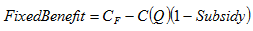
(2) Where CF denotes the cost of purchasing a traditional vehicle, which is treated as constant in the simulation, Subsidy denotes the per cent of the purchasing cost of an AFV that the government will pay to the driver agent, and C(Q) denotes the cost of an AFV when the cumulative production is Q.
- 3.16
- With more driver agents switching to AFVs, the cost of an AFV decreases according to the technological learning effect (Arrow 1962), described by Eq. (3)
(3) where C0 denotes the initial cost of purchasing an AFV, Q denotes the cumulative production/purchasing[4], b is the elasticity of investment cost with regard to cumulative production and it is easy to prove that 1−2−b (which is called technological learning rate) is the percentage of cost reduction when cumulative production doubles.
- 3.17
- The driver agents' VariableBenefit is calculated with Eq. (4)
(4) where EF denotes a traditional vehicle's fuel cost per kilometre and E denotes an AFV's fuel cost per kilometre. In our current version of the model, EF and E are defined as a constant value. From the long run, EF and E might be dynamic as the price of gasoline and electricity are changing, which will be considered in our future work.
- 3.18
- In the model, Beliefspace&Volume is calculated with Eq. (5)
(5) where B denotes the social value of using an AFV, and it is defined as a driver agent's average annual income (see Schwoon 2008), MF denotes the monthly maintenance cost of a traditional vehicle, M0 denotes the initial monthly maintenance cost of an AFV, nt denotes the number of driver agents using AFVs at time t, and N is the total number of driver agents.
- 3.19
- One step in the model represents one month. A driver agent remembers the availability of the filling stations from his/her previous driving experiences, and thus, the WorryFactor is not only dependent on his/her worry in the current step but is also dependent on his/her worry in previous steps. The WorryFactor is calculated as the weighted average of worry in the current and previous steps (a total of 12 steps, i.e., one year), and the closer to the current step, the larger the weight.

(6) where Wj represents the weight of worry at step j, which is calculated with Eq. (7).
(7) where a ∈ (0,1) is the weight for the current step. If a is set as 0.2, the weight for the current step is 20%, and the weight for one year ago is less than 2%.
- 3.20
- Worryj in Eq. (6) denotes a driver's worry about the availability of refuelling at step j, which is calculated with Eq. (8):

(8) where StationDisancenj means the distance between the n th refuelling station and the next station during the driver agent's trip at step j, DistanceTravledj denotes the total distance that the driver agent drives at step j, and λ is a design parameter, which is used to transfer worries into currency. Its meaning can be thought of as the expected loss in worry for each kilometre. The DWD (Don't Worry Distance) depends on the technology unique to a vehicle as well as the driver agents' feelings on the maturity of the vehicle technology. For example, the refuelling range of a traditional vehicle is higher than that of an AFV, and the traditional vehicle technology is more mature than an AFV technology; therefore, the DWD for the traditional vehicles is larger than the DWD for the AFVs.
Station owner agents
- 3.21
- A station owner agent will consider establishing a new filling station if he/she finds that there are many (i.e., above a threshold) AFVs passing by a location. The establishment of new filling stations will influence a driver's WorryFactor, and thus, the utility of using an AFV. Once a station is built, it will be operated for at least 6 months, and after that, it will be closed if the number of AFVs passing by it drops to less than a threshold.
- 3.22
- Following the SS model, a station owner agent's utility for building a new filling facility is defined with Eq. (9)
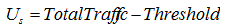
(9) where Us denotes a station owner's utility, TotalTraffic is the number of AFVs passing through a location during a certain time period, and Threshold is a number indicating that, when there is a sufficient number of AFVs passing through a filling station, the station can make a profit and therefore survive. For a location, the TotalTraffic is determined by all driver agents' decisions on adopting AFVs as well as their driving routes which can be generated with the method introduced in section 3.7.3. We assume that a station owner agent will observe the number of AFVs passing through a location for 12 steps (i.e. 12 months), and the TotalTraffic is calculated as the weighted average over the 12 steps. The weight for each step is calculated with Eq. (6); thus, larger weight is placed on steps closer to the current step.
- 3.23
- Whether a filling station can make a profit and survive depends not only on how many potential consumers there are (i.e. the number of AFVs passing through the station) but also on the number of competitive stations. In our model, the Threshold is a function of the total number of AFV refuelling stations as well as the distance to its neighbouring AFV stations, as shown in Eq. (10)[5].
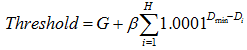
(10) where G denotes the total number of existing AFV filling stations, Dmin denotes the minimal distance between two neighbour nodes overall the road network. Here "nodes" means nodes of the road network. A road network is denoted with many nodes and links (or edges) in a GIS. Dmin indicates the shortest link (or edge) in the road network. It does not mean the minimal distance between two filling stations. Di denotes the distance between the location at which a new filling station is considered to be built and its i th neighbouring filling station, and β is a design parameter signifying the weighted distance to its neighbouring stations. It follows from Eq. (10) that more total AFV filling stations as well as more and closer neighbouring stations result in a higher Threshold. In our model, we set β=10, which means that a very close neighbouring filling station will increase the Threshold by 10. With Eq. (10), two filling stations can be in direct neighbourhood, if the number of AFVs passing through their location is large enough, i.e., larger than the threshold calculated with Eq. (10) and thus both of them can have good business to survive. Eq. (10) reflects our stylised assumption that each filling station needs a certain number of customers to survive.
- 3.24
- When the Us for a location is positive, a filling station for AFVs will be built there. Once a new filling station is built, it will be operated for at least 6 steps. After 6 steps, if Us becomes negative, then the station will be closed.
- 3.25
- With the agent-based model, we can run computer simulations. A successful adoption process could be described as the following. At the beginning, there are few pioneer adopters of AFVs. With the initial filling stations organised by the government, the technological learning effect causes the FixedBenefit to increase, and more drivers will adopt AFVs. As a result, more filling stations will be built, further decreasing the drivers' WorryFactor and encouraging more drivers to adopt AFVs. More drivers adopting AFVs will result in greater rate of technological learning and the establishment of more filling stations, thus causing a beneficial cycle of the adoption of AFVs. Adoption could also devolve into a cycle of negative feedback and fail if the effect of technological learning is too weak, if government subsidies are insufficient, or if the layout of initial filling stations is not appropriate.
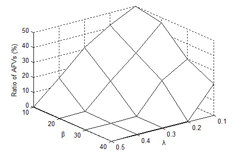
Figure 3. Adoption of AFVs at step 50 with different β and λ - 3.26
- In the model introduced above, λ in Eq. (8) and β in Eq. (10) are two design parameters, which are parameterised ad-hoc. Figure 3 plots the ratios of AFVs at step 50 with different values of λ and β, with other parameters set as the same[6]. From Figure 3 we can see that, with the increase of λ, the diffusion of AFVs becomes slower, this is because a larger λ denotes a bigger weight to concerns on the availability of AFVs' filling stations, thus driver agents will be more reluctant to adopt AFVs. Figure 3 also shows that with the increase of β, the diffusion of AFVs becomes slower. This is because with a larger β, the threshold for a filling station to survive becomes higher, and thus the diffusion of filling stations becomes slower which result in slower diffusion of AFVs.
Linking the agent-based model with a GIS and social and economic background
-
Techniques and solutions
- 3.27
- In the original SS model, agents live in a stylised space defined by a square, and the road network is defined by intersecting lines that form right angles. Most of the driver agents' driving trips are for commuting. The driver agents' homes and work places are initialised randomly in the square space. For each driver agent, his commuting trip is set to be the shortest path between his home and work place. The driver agents' other driving trips are set from their homes to an attraction, e.g. a shopping mall. The stylised model can explain the complexity of the adoption process, but the simulations are far from realistic scenarios because they are not linked with a real social-economic background. To help decision makers find a close-to-optimal layout of the initial filling stations, our training system links the agent-based model with a real city/area's road network in a GIS as well as the city/area's social and economic background.
- 3.28
- In recent years, with the fast development of GISs, a large amount of spatial data is stored digitally in various GISs. Integrating these spatial data into agent-based models is an advance of the ABM approach, and researchers have focused increasingly greater attention to this effort (Gilbert 2007). The integration of ABMs and GISs still faces a large number of challenges, and the primary issue is that the software platform and technology of ABMs and GISs have been developed independently (Stanilov 2011).
- 3.29
- The integration of ABMs and GISs can be classified into two types, grid-based integration and vector-based integration. The first type of integration is relatively simple. It replaces the square space with a polygon denoting an area's shape, but the main elements in the space are still grids. Most of the current integrations of ABMs and GISs are of this type. The second type integrates vectors denoting the space topology into an ABM. This type of integration is more complex, and it usually demands very large computational requirements (Stanilov 2011).
- 3.30
- A city/area's road network in a GIS is stored mostly as vectors. With Repast (North et al. 2013) as the ABM platform, and with ArcGIS (ESRI 2004) as the GIS platform, we explored a vector-based solution for linking the SS model with a real-road network. In our solution, Repast and ArcGIS work mostly independent of each other, and all of the communications between Repast and ArcGIS are realised through reading and writing operations on shapefiles in which spatial vectors are stored as two-dimensional tables. The data exchange works in both directions between Repast and ArcGIS at each simulation step. In the agent-based model, new filling stations will be established and some old ones might be closed at each step, which will influence driver agents' utility. So at each step, Repast will obtain the position of all agents from ArcGIS's shapefile and write back the changing of station owners' position to shapefile. And of course, visualisation is another reason for getting back to ArcGIS.
A simple method for the driving trip generator
- 3.31
- Various existing traffic forecasting methods (e.g. 1987; Tsekeris & Stathopoulos 2006; Chrobok et al. 2005; Dia 2001) can be used to generate the driving trips in an area for the agent-based model. These methods commonly require very intensive data collection and analysis. Considering that our model is not intended for traffic management or planning, we developed a simpler method as an alternative option (in addition to traditional methods) for users to generate driving trips for the ABM (Ma et al. 2014). The method does not require extensive work to be performed on the data. It uses widely available social, economic, and spatial data as inputs to generate driving trips in an area. The method is described below.
- 3.32
- Cities/areas are commonly composed of several districts, and statistical data, such as GDP and population size, are often widely available at the district level. Thus, our method uses statistical data at this level to generate driving trips. Compared with trips for other purposes, such as shopping and leisure, commuting trips are more fixed, both in terms of time and space. As shown in Table 1, commuting trips in a city/area can be divided into four major types resulting from the combinations of one's home and work place locations. For different cities/areas, the proportion of the four types of commute in Table 1 could be different.
Table 1: Spatial types of commutes Type Location of home Location of work place Within-commute Centre Centre Inward-commute Suburb Centre Reverse-commute Centre Suburb Lateral-commute Suburb Suburb - 3.33
- Several driver agents' homes might be very close, for example, in the same community. In the simulation, we simply assume that they are living in the same location, called a living quarter. Similarly, several driver agents' work places might be very close, for example, in the same business park. In the simulation, we also simply assume that they are working in the same location, called a working quarter. As shown in Figure 4, our method of generating commute driving trips starts by calculating the number of living quarters and working quarters in each district, using population and GDP data.
- 3.34
- The number of living quarters in each district is calculated with Eq. (11)
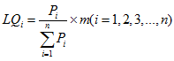
(11) where LQi denotes the number of living quarters in the ith district of a city, Pi denotes the resident population in the ith district, m denotes the total number of living quarters in the city/area, and n denotes the number of districts in the city.
- 3.35
- The number of working quarters in each district is calculated with Eq. (12)
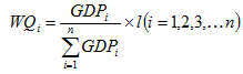
(12) where WQi denotes the number of working quarters in the ith district, l denotes the total number of working quarters, and GDPi denotes the ith district's GDP.
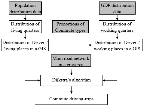
Figure 4. Method of generating a commute driving-trip. Rectangles with bold frames and gray background denote the inputs used to generate the commuter driving trips - 3.36
- After obtaining the number of living and working quarters in each district, they are placed in each district randomly in a GIS digital map. Then, each driver agent is randomly assigned a living quarter, and following the proportion of the four commute types in Table 1, each driver agent is randomly assigned a working quarter. Dijkstra's algorithm (Dijkstra 1959) is applied for each driver agent to decide his/her commute route[7]. Dijkstra's algorithm is one of the most popular algorithms for finding the shortest path between two locations, and it is widely used in many GIS systems.
- 3.37
- In addition to driving trips for one's commute, driving trips for other purposes are generated from the driver agents' home and attractions such as shopping malls. Additionally, there are also randomly chosen driving trips. For each step, which denotes one month in our model, we assume that there are 20 two-way trips for one's commute, and a number of trips to attractions that follow a Poisson distribution with a mean of 8 and an upward limit of 10.
- 3.38
- We tested the method with data from Shanghai, one of the largest cities in China, and found the commute times produced by the method were in close agreement with survey results (see more details in the case study in section 5), which provides some validation of the potential usefulness of the method[8].
Getting a close-to-optimal solution
- 4.1
- Users of the training system can attain a close-to-optimal solution either by a trial-and-error method or with the help of a genetic algorithm. The training system provides a GUI through which a user can put (in this case, 10) initial filling stations in a map by inputting their coordinates manually. After setting a layout of the initial refuelling stations, the user can run the simulation to generate an adoption scenario of the AFVs. The user can set as many different layouts as he/she wants, and generate different adoption scenarios. By comparing these scenarios, the user can select the layout, which generates the fastest adoption of AFVs. If a decision-maker already has a design of layout in his/her mind, he/she can use the training system to test whether the design can generate a successful adoption of AFVs, and after the testing, he/she might modify a portion of the design and do testing again.
- 4.2
- In additional to setting the initial layout manually, we also developed a GA to help users to set an initial layout with close-to-minimal concerns (on refuelling) of all driver agents. The GA treats a layout as a genome, and the probability that a layout is selected as the parents for the next generation is calculated with Eq.(13).
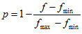
(13) where f is the average of all potential adopters' concerns with the layout, and fmax is the maximal average of all potential adopters concerns with all layouts in the same generation, and fmin is the minimal average of all potential adopters' concerns with all layouts in the same generation. With Eq. (13), for smaller average concerns of a layout, there is a larger probability that the layout is selected as the parents for the next generation. The GA will be terminated with one of the following conditions: (1) the minimal average concerns with a series of generations are stable; (2) the number of iterations with the GA reaches a predefined number.
- 4.3
- The initial layout generated with the GA does not have to be the best one. It is an option, which is not generated with users' intuition but with a special objective (minimal concerns of all potential adopters) and might help the adoption of AFVs. Users can use it as a starting layout to find their satisfying one with simulation scenario analysis described in the first paragraph of this section.
A case study with Shanghai
- 5.1
- Sponsored by the Shanghai Science and Technology Committee and the Shanghai Education Committee, we performed a study of the initial layout of fast-charging or battery-changing stations for electric vehicles in Shanghai.
- 5.2
- Shanghai is one of the biggest cities in China. Its economy and facilities are well developed. In 2011, Shanghai became the first city in China to start demonstration projects of plug-in electric vehicles. It has the potential to be selected as the adoption centre for AFVs. With this study, we aim to find the optimal layout of initial filling stations for electric vehicles based on the concept of fast-charging or battery-changing stations. The main purpose of presenting this case study is to demonstrate how the training system can help the decision makers find a close-to-optimal layout. As a result, we do not implement intensive data collections to generate driving routes in Shanghai; instead we use the simple method introduced in para. 3.31 to generate driving routes.
- 5.3
- Shanghai is composed of 19 districts; we assume that each district has an attraction located at its centre. We also assume that there are 400 living quarters and 400 working quarters in Shanghai. Here, we did not use the real number of living and working quarters in Shanghai because the agent-based model does not aim to replicate reality; instead, it uses a small number of agents to represent all of the drivers in Shanghai. In effect, the distribution of the representative agents is most important and not the number of actual drivers in reality. The numbers of living and working quarters in each district were calculated with Eq. (11) and Eq. (12), with the statistical data taken from the Shanghai Statistics Year Book (2009). We assume that each living quarter is the location of 20 driver agents' homes.
- 5.4
- Table 2 gives the proportion of different commuting trip types from the latest transportation survey in Shanghai in 2009 (SFTS 2009). Then, using the method introduced in Section 3.7.3, we generate the driving trips in Shanghai.
- 5.5
- According to the latest transportation survey, the average speed on Shanghai's main roads during commuting periods ranges from 15 to 21 kilometers/hour (SFTS 2009). We used the median speed, 18 kilometers/hour, to calculate the driver agents' commute time, and we found that the mean commute time of 10 simulations is 47.3 minutes, which is close to the 46 minutes reported in the survey. The distribution of the commuting times in our simulations is also in agreement with the results of another survey, performed by Wang and Gan (2010).
Table 2: The percentages of commutes in Shanghai in 2009 (%) Origin Destination Center Suburbs Center 92.9 7.1 Suburb 12.1 87.9 - 5.6
- We use Shanghai's main road network for our simulation. The road network includes more than 800 pieces of road and more than 500 nodes.
- 5.7
- Based on a survey on the traditional and electric vehicles in the market, we performed the following estimation for traditional vehicles and electric vehicles in the model. The cost of a traditional vehicle is assumed to be 25,000 US$, its annual maintenance cost is 150 US$, and its fuel cost per kilometre is 0.1 US$. The initial price of an electric vehicles is 40,000 US$, its initial annual maintenance cost is 300US$, and its energy cost per kilometre is 0.025US$ (i.e. 25% per cent of a traditional vehicle). The social value of using an AFV is set according to the average annual income, which is 7000 US$. The technological learning rate of the electric vehicle is assumed to be 10%.
- 5.8
- In Shanghai, the subsidy from the government for an electric vehicle is approximately 40% of the total price (including a free license plate, which is otherwise priced by a monthly auction, and a reduced purchasing tax). The driver agents' DWD is set to 11 km. In addition, λ in Eq. (6) is set to 500 US$[[9]], which indicates the expected loss of worry for each kilometre, and only 40 driver agents are designated as adopters of AFVs at the beginning of the simulation. Suppose the government plans to build 10 initial filling stations, then what type of layout can induce a successful adoption process of electric vehicles?
- 5.9
- The time period for each driver agent to update his/her vehicle follows a normal distribution with a mean of four years (48 steps) and a standard deviation of one year (12 steps).
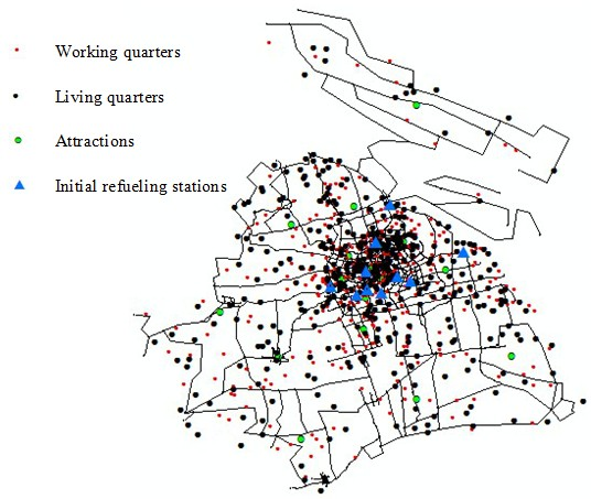
Figure 5. Shanghai main road network and the distribution of attractions, living quarters, and working quarters in the agent-based model - 5.10
- Figure 5 depicts the main road network of Shanghai, the distributions of living quarters, working quarters, and attractions as well as the initial filling stations.
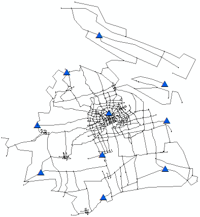
a. Dispersed layout 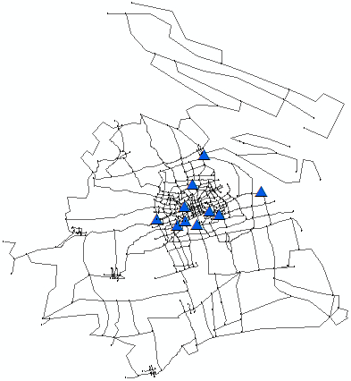
b. Concentrated layout 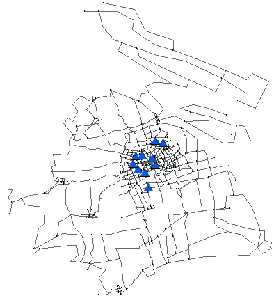
c. GA layout Figure 6. Three different layouts of initial filling stations 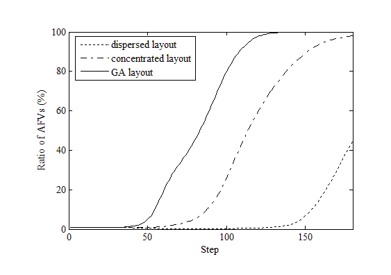
Figure 7. Adoption of electric vehicles with different layouts of initial filling stations - 5.11
- Figure 6 plots three different layouts of the 10 initial filling stations. The first two layouts (Figure 6a and Figure 6b) are set randomly. In Figure 6a, the 10 initial filling stations are put randomly over the whole Shanghai. In Figure 6b, the 10 initial filling stations are put randomly in the centre of Shanghai. Figure 6c is a layout generated with the GA algorithm introduced in section 4.
- 5.12
- Figure 7 plots the adoption of the electric vehicles with the three different layouts. From Figure 7 we can see that with the layout generated with the GA, the diffusion of the AFVs is about two years (24 simulation steps) earlier than that with the second layout and about eight years (96 simulation steps) earlier than that with the first layout. This comparison can somehow validate our belief that reducing driver agents' initial total concerns on refuelling can help the diffusion of AFVs. The GA helps decision makers find the layout that produces close-to-minimal average concerns for all potential adopters. Decision makers can generate several initial layouts with the GA, as shown in Figure 8, which plots the decreasing of average concerns when applying the GA with different populations at each generation. And then decision makers can test these layouts with the agent-based model and select the one that can induce the most successful adoption.
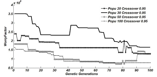
Figure 8. Decrease of the average concerns using the GA - 5.13
- In this study, we assumed the number of initial filling stations is 10. By increasing efforts to promote the adoption of electric vehicles through fast-charging or battery-changing stations, the number of initial filling stations would be larger. What we have presented here is mainly an illustration of how the training system can help decision makers find the appropriate layout. Users of the system can explore close-to-optimal layouts with different situations and for different cities/areas.
Concluding remarks
- 6.1
- Adoption of AFVs is a complex process involving heterogeneous actors. It is difficult to identify an optimal layout of initial filling stations for alternative fuel vehicles in a city/area with traditional operational optimisation or equilibrium analysis. This paper presents a training system for finding a close-to-optimal layout by integrating an agent-based model with a GIS and the social and economic background of a city.
- 6.2
- In addition to the layout of the initial filling stations, adoption of AFVs will also be influenced by other factors, with some of them addressed by the model introduced in this paper, e.g. (technological learning potential, government subsidies, etc.). To focus on solving the problem of finding a close-to-optimal layout, the current study assumes other factors are already known. In reality, even with a good layout of the initial filling stations, the widespread adoption of AFVs could fail as a result of other factors. Studying the influences of these other factors is beyond the scope of this paper.
- 6.3
- Although the agent-based model and simulations presented in this paper attempt to be more realistic with the integration of a real-road network as well as incorporation of social and economic data, they do not purport to accurately replicate reality. It is beyond any research project's capacity to know each driver's extract driving routes in a city/area because there could be millions of possible routes. What the agent-based model and simulation in this work did was to capture the spatial distributions of all drivers' routes with representative agents. As a result, the training system described here can help expand decision makers' imaginations as well as enhance their intuition of the design for appropriate layout of initial filling stations.
- 6.4
- Traditional approaches for locating new filling stations mainly consider the traffic flow and external constrains such as far away from sparks, and they pay little attention to the co-diffusion process of AFVs and their filling stations. The model and approach presented in this paper focus on the co-diffusion process of AFVs by explicitly modelling the interactions among driver agents and station owner agents which are very important during the taking off of AFVs' diffusion. The model and study mainly focused on developing a training system by linking a stylised agent-based model with GIS and social-economic background of a specific city. The agent-based model itself was kept as simple as previous study. For example, the current model does not consider the dynamics of gasoline price and governments' subsidy. The driver agents in current model are only characterised by their driving routs. In reality, driver agents' income, age, gender, education, and so on, might influence their decision on adopting AFVs. The training system presented in this paper is a prototype system. It provides a platform for adding further realities into the model and simulations. In the future work, we would add external (or environmental) dynamics into the model, such as the dynamics of gasoline price, governments' dynamic subsidy, and so on. We would also model driver agents' heterogeneity in terms of their income, age, gender, education, and so on. In addition, in future work, we would develop more complicated GA methods for getting the close-to-optimal layout of initial filling stations. We plans to develop a GA-method which allow decision makers to trade off between cost and effect of the layout, and we also plan to develop a GA method which nests the agent-based simulation process into the genetic algorithm and use the adoption result as a measure of a given layout's fitness. In the current model, whether a filling station can survive is simply determined by the number of AFVs passing through it. In the future work, we would consider a more detailed economic evaluation on the investment cost, operation cost, and revenue of filling stations.
Acknowledgements
- This research was sponsored by the National Nature Science Foundation of China (project no. 70901026 and 71125002), the Ministry of Education of China (project no. NCET-09-0345), the Shanghai Education Committee (project no. 08SG30), and the Shanghai Science and Technology Committee (Pujiang project 2009). These funding sources had no involvement in the study except providing financial support.
Notes
-
1 See http://www.teslamotors.com/supercharger
Archived at: http://www.webcitation.org/6Ok93xxwD
2 For such electric vehicles, it is better to install recharging facilities in parking places.
3 With a greater adoption of one type of AFVs, there will be more service centers for the maintenance of that type of AFVs. Thus, the maintenance will be more convenient, and the price of maintenance might decrease with competition.
4 In the model, we simply assume that the supply of and demand for AFVs are the same.
5 For a specific kind of AFVs, it is better to do a detailed study of the economics of establishing a new refueling station, which will be discussed in our future work.
6 See more details in section 5. In the simulations reported in Figure 3, the layout of initial filling stations is set as in Figure 6b.
7 In reality, a driver might not select the shortest path. In this simplified method, we follow the SS model because the method is not used for traffic forecasting but for generating driving routes of representative agents.
8 With the method, we also did another case study with Beijing, which also provides some validation of the potential usefulness of the method (Ma et al. 2014).
9 We adopt the idea of average month income (see Schwoon 2008)
References
-
ARROW, K.J. (1962). The economic implications of learning by doing. Review of Economic Studies. 29(3): 155–173. [doi:10.2307/2295952]
ARTHUR, W.B. (1999). Complexity and the economy. Science. 284(5411): 107–109. [doi:10.1126/science.284.5411.107]
AXELROD, R. (1997). Advancing the art of simulation in the social sciences. R. Conte, R. Hegselman, P. Terna (eds.). Simulating Social Phenomena, Springer, 21–40. [doi:10.1007/978-3-662-03366-1_2]
BEYRER, C., Baral, S.D., Van Griensven, F., Goodreau, S.M., Chariyalertsak, S., Wirtz, A.L., & Brookmeyer, R. (2012). Global epidemiology of HIV infection in men who have sex with men. The Lancet. 380(9839), pp. 367–377. [doi:10.1016/s0140-6736(12)60821-6]
BUNN, D.W., & Oliveira, F.S. (2001). Agent-based simulation - An application to the new electricity trading arrangements of England and Wales, IEEE Transactions on Evolutionary Computation (5) , pp. 493–503. [doi:10.1109/4235.956713]
CHINA'S STATE COUNCIL. (2012). Developing Plan of Energy-Saving and Alternative-Energy Vehicle Industry from 2012 to 2020.
CHOI, J.K., & Bowles, S. (2007). The coevolution of parochial altruism and war. Science, 318 (5850), pp. 636–640. [doi:10.1126/science.1144237]
CHROBOK, R., Kaumann, O., Wahle, J., & Schreckenberg, M. (2005). Different methods of traffic forecast based on real data. European Journal of Operational Research, 155: 558–568. [doi:10.1016/j.ejor.2003.08.005]
DELRE, S.A., Jager, W., & Janssen, M.A. (2007). Diffusion dynamics in small-world networks with heterogeneous consumers. Computational and Mathematical Organization Theory 13 (2) , pp. 185–202. [doi:10.1007/s10588-006-9007-2]
DIA, H. (2001). An object-oriented neural network approach to short-term traffic forecasting. European Journal of Operational Research, 131: 253–261. [doi:10.1016/S0377-2217(00)00125-9]
DIJKSTRA, E. (1959). A note on two problems with graphs. Numerical Mathematics. 1: 267–271.
DUFFUS, L.N., Alfa, S.A., & Soliman, A.H. (1987). The reliability of using the gravity model for forecasting trip distribution. Transportation, 14 (3):175–192. [doi:10.1007/BF00837528]
ESRI. (2004). ArcGIS Engine Developer Guide.
FARMER, J.D. & Foley, D. (2009). The economy needs agent-based modeling. Nature, 460 (6): 685–686. [doi:10.1038/460685a]
GILBERT, G.N. (2007). Agent-Based Models, SAGE . 68–90.
GRIMM, V., Berger, U., Bastiansen, F., Eliassen, S., Ginot, V., Giske, J., Goss-Custard, J., Grand, T., Heinz, S.K., Huse, G., Huth, A., Jepsen, J.U., Jørgensen, C., Mooij, W.M., Müller, B., Pe'er, G., Piou, C., Railsback, S.F., Robbins, A.M., Robbins, M.M., Rossmanith, E., Rüger, N., Strand, E., Souissi, S., Stillman, R.A., Vabø, R., Visser,U., & DeAngelis, D.L. (2006). A standard protocol for describing individual-based and agent-based models. Ecological Modelling, 198: 115–126. [doi:10.1016/j.ecolmodel.2006.04.023]
LEE, K.C., & Lee N. (2007). CARDS: Case-Based Reasoning Decision Support Mechanism for Multi-Agent Negotiation in Mobile Commerce. Journal of Artificial Societies and Social Simulation. 10 (2), 4, https://www.jasss.org/10/2/4.html.
MA, T.J,Zhu Y.,Liu, P.P., and Chi, C.J. (2014).A simulation method to generate commute trips—for agent-based modeling on co-diffusion of alternative fuel vehicles and their filling stations. Simulation: Transactions of the Society for Modeling and Simulation International. 90(5):560-569. [doi:10.1177/0037549714530780]
NORTH, M.J., N.T. Collier, J. Ozik, E. Tatara, M. Altaweel, C.M. Macal, M. Bragen, & P. Sydelko. (2013). Complex Adaptive Systems Modeling with Repast Simphony. Complex Adaptive Systems Modeling, Springer, Heidelberg, FRG. http://www.casmodeling.com/content/1/1/3.
PALMER, R.G., Arthur, W.B., Holland, J.H., LeBaron, B., & Tayler, P. (1994). Artificial Economic Life: A Simple Model of a Stockmarket, Physica D 75, 264–274. [doi:10.1016/0167-2789(94)90287-9]
SCHWOON, M. (2008). Learning by doing, learning spillovers and the diffusion of fuel cell vehicles. Simulation Modelling Practice and Theory. 16:1463–1476. [doi:10.1016/j.simpat.2008.08.001]
SFTS (Shanghai Fourth Transportation Survey). (2009). http://sh.eastday.com/chztl/4thjtsurvey/.
Archived at: http://www.webcitation.org/6Ohrl6L3h.
SHANGHAI STATISTICS YEAR BOOK. (2009). http://www.stats-sh.gov.cn.
Archived at: http://www.webcitation.org/6OjFjNMjg.
SHI, J.Y., Ren, A.Z., & Chen, C. (2009). Agent-based evacuation model of large public buildings under fire conditions. Automation in Construction. 18 (3): 338–347. [doi:10.1016/j.autcon.2008.09.009]
STANILOV, K. (2011). Space in agent-based models, Agent-Based Models of Geographical Systems, Springer. 253–269.
STEPHAN, C., & Sullivan, J. (2004). An agent based hydrogen vehicle/infrastructure model. Proceedings of the Congress on Evolutionary Computation, IEEE, New York. 1774–1779. [doi:10.1109/cec.2004.1331110]
STRADER, T.J., Lin, F.R., & Shaw, M.J. (1998). Simulation of Order Fulfillment in Divergent Assembly Supply Chains. Journal of Artificial Societies and Social Simulation. 1 (2), 5 https://www.jasss.org/1/2/5.html
TSEKERIS, T., & Stathopoulos A. (2006). Gravity models for dynamic transport planning: Development and implementation in urban networks. Journal of Transport Geography. 14: 152–160. [doi:10.1016/j.jtrangeo.2005.06.009]
US DEPARTMENT OF ENERGY (DOE). (2013). EV Everywhere Grand Challenge Blueprint.
WANG, W., & Gan, H. (2010). Car or public transit? – Analysis on travel mode choice behavior. Urban Transport of China. 8 (3): 36–40 (in Chinese).
WOOLDRIDGE, M., & Jennings, N. (1995). Intelligent agents: Theory and practice. Knowledge Engineering Review. 10 (2): 115–152. [doi:10.1007/3-540-58855-8]