
 Abstract
- During the last thirty years education researchers have developed models for judging the comparative performance of schools, in studies of what has become known as "differential school effectiveness". A great deal of empirical research has been carried out to understand why differences between schools might emerge, with variable-based models being the preferred research tool. The use of more explanatory models such as agent-based models (ABM) has been limited. This paper describes an ABM that addresses this topic, using data from the London Educational Authority's Junior Project. To compare the results and performance with more traditional modelling techniques, the same data are also fitted to a multilevel model (MLM), one of the preferred variable-based models used in the field. The paper reports the results of both models and compares their performances in terms of predictive and explanatory power. Although the fitted MLM outperforms the proposed ABM, the latter still offers a reasonable fit and provides a causal mechanism to explain differences in the identified school performances that is absent in the MLM. Since MLM and ABM stress different aspects, rather than conflicting they are compatible methods.
- Keywords:
- Agent-Based Modelling, Differential School Effectiveness, Multilevel Modelling, Peer Effects, Teacher Expectation Bias
Introduction
- 1.1
- During the last thirty years education researchers have studied why some schools differ significantly in terms of their effectiveness for particular pupil groups, in studies of what has become known as differential school effectiveness (Coleman 1966; Nuttall et al. 1989; Reynolds et al. 2011; Sammons et al. 1993). These variable-based models, which have achieved great sophistication, allow the researchers to identify the extent to which schools improve pupils' educational attainment. Among these models, Multilevel Models (MLM) are very popular, since they allow the analysis of data that have a hierarchical structure, with two or more 'levels', such as pupils and schools (Paterson & Goldstein 1991). However, despite their sophistication, variable-based models such as MLM generally do not provide causal explanations (Hedström & Swedberg 1996). This is because variable-based models cannot represent the social interactions and actors that together constitute the structures in which they are embedded (Cederman 2005; Macy & Willer 2002).
- 1.2
- Whether a MLM (or any statistical model) is able to identify causal effects depends largely on the availability of longitudinal data on likely causal influences, controlled experiments with very restrictive conditions and detailed knowledge about the underlying processes (Carrington et al. 2005). Of course, such information, which would allow researchers to formulate more complex models – truly closer to causal models – is rarely available. In the absence of such data, MLM are still well suited to identify statistical differences among groups of pupils, but they cannot explain why those differences might emerge in the first place, since they do not uncover the generative mechanisms that bring them about. When researchers want to understand why some social phenomenon emerges but they do not have access to precise longitudinal data, agent-based modelling (ABM) might be the best alternative to complement the conclusions extracted from a variable based model (Gilbert 2008). Researchers can use ABM to explain differential school effectiveness by focusing on the dynamics of the social networks shaped by pupils' interactions within and outside the school. The use of ABM in combination with variable based models in social (Manzo 2007) and educational research (Maroulis et al. 2010b) has been increasingly employed during the last few years. For instance, Maroulis et al. (2010a) developed an agent-based model that, using data from Chicago public schools, addressed the difficulties in evaluating the impact of choice-based reforms in education. Montes (2012) calibrated his agent-based model with empirical data to study the causal implications of the so called "same-race effect" between pupils and teachers on the United States educational achievement trends. Manzo (2013) developed an empirically calibrated agent-based model to show that the observed French stratification of educational choices could be accounted for by network-based mechanisms (e.g., homophilic dyadic interactions taking place within friendship networks). More recently, Stoica and Flache (2014) developed a model of school segregation by studying whether ethnic preferences have a similar effect on school segregation as they have on residential segregation and how this is affected by a simultaneous preference for a short distance between home and school.
- 1.3
- These investigations show that ABM is a method that enables researchers to explore and understand in silico the macro-level consequences of individuals' behaviours and interactions. By so doing, the researcher explicitly proposes and formalises a mechanism-based explanation of the observed macroscopic phenomenon (Hedström 2005). Thus, ABM aims to be explanatory, while MLM is a sophisticated way of description and hypotheses testing. Since the two methods share a similar understanding of social reality, they complement each other in their diagnostic and explanatory capabilities.
- 1.4
- The primary focus of this paper is to compare MLM and ABM in terms of their predictive and explanatory power. This is done by fitting a MLM and by formalising an ABM to explain differences in school effectiveness. Therefore, this is a methodological investigation about (as we argue here) two different but complementary research techniques. However, models in general and agent-based models in particular must be based on rigorous or at least plausible theories and hypotheses, since any model being constructed is one concrete realisation of some prior assumptions about how individuals act and interact in some specific setting (Wu & Sun 2005). We cannot avoid being explicit on the theoretical foundations of our computational model, which aims to explain the observed differences in school effectiveness. For this reason, the paper describes in detail the proposed ABM and the specific theory specified by it, designed to understand peer and teacher expectations bias effects on educational attainment. Having formalised the generative mechanism that, we claim, could bring about the observed differences in school effectiveness, we calibrate the agent-based model empirically, estimating and setting its initial conditions, so that the results from the multilevel and the agent-based model can be compared. It is shown that, although the fitted MLM outperforms the proposed ABM in the accuracy of its quantitative predictions, the latter still offers a reasonable fit and, in addition, provides a causal mechanism to explain differences in school performance that is absent in the MLM. A mechanism-based explanation might thus complement the statistical differences among groups found using MLM.
- 1.5
- Because the primary goal of this article is to compare and to find compatibilities between these two methods, we are not interested in identifying precisely the underlying processes that causally explain differences in school effectiveness. Hence, the mechanism we implement as the model micro-specification must be understood as a candidate mechanism-based explanation, a provisional hypothesis that, although sufficient to generate the observed differences, should be subject to further empirical testing (Epstein 1999). We begin this paper with a brief account of MLMs in education research. We describe the data we are using and fit a MLM to evaluate possible group effects and the extent to which differential school effectiveness is manifest in the data. Then we present an ABM to explain differential school effectiveness, describing the model entities, interactions and main dynamics. The last part of the paper compares the two modelling techniques, evaluating their predictive power. The paper concludes with some remarks about the two modelling techniques.
Multilevel Modelling and School Effectiveness Research
- 2.1
- In the context of educational research, MLM were developed to adjust simple comparisons of school mean values by using measures of pupils' prior achievement and other control variables. These comparisons aimed to take account of selection and other procedures that are associated with pupils' achievement and are unrelated to any effect that the schools themselves may have on achievement (Goldstein et al. 2007; Steele et al. 2007). The extent to which the school is 'adding value' to the education process is determined by using statistical models that include these non-school factors. The objective is to isolate statistically the contribution of schools from these factors (Meyer 1997). This approach, of measuring school effectiveness in terms of the value the school adds to the education process, has been reinforced by broader efforts to hold schools accountable (Ladd & Walsh 2002). One manifestation of this trend is the proliferation of rankings based on such measurements, which are designed to provide parents and taxpayers with information about the quality of schools.
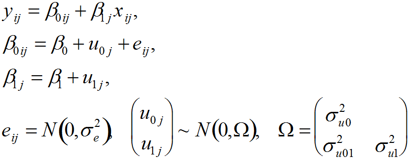
A multilevel model
- 2.2
- When a MLM is used, it is assumed that the group level makes a difference that explains part of the total variance of the dependent variable (Gelman & Hill 2006). A simple two-level, random intercept model based on data from a random sample of schools can be written as follows, where subscript i refers to the pupil, and j to the school:
yij = β0 + β1x1j + eij, uj ∼ N(0,σu2), eij ∼ N(0,σu2), (1) where yij and xij are the response variable and prior attainment respectively, and uj is an underlying school effect (which is associated with school organisation, teaching, etc.). This model assumes that eij and uj are uncorrelated and also uncorrelated with any explanatory variable, i.e. it assumes that any possible dependences that may result from, for example, school selection mechanisms are accounted for. Posterior estimates ûj with associated confidence intervals are typically used to rank schools in 'league tables' or used as 'screening devices' in school improvement programmes.
- 2.3
- Model 1 can be elaborated by introducing further covariates such as socio-economic background or peer group characteristics, to make additional adjustments, satisfy the distributional assumptions or investigate interactions. In addition, it is typically found that models such as Model 1 require random coefficients, where, for example, the coefficient of prior achievement varies randomly across schools. In this case, using a more general notation, we have
(2) - 2.4
- The Multilevel Model 2 may also be extended to include further levels of hierarchy, such as education board or authority, and random factors that are not contained within a simple hierarchy, such as area of pupil residence or school attended during a previous phase of education. Such designs are known as 'cross-classifications' (Leckie 2009). Both model 1 and the multilevel model 2 are structurally similar to those used by economists, who typically approach the challenge of measuring school effectiveness within the context of a standard education production function (Hanushek & Taylor 1990). In these production functions, the achievement of student i in year t is a function of the student's achievement in the prior year, the school characteristics, the student's family background characteristics that might affect achievement, and, to the extent possible, all the factors out of the control of the school's faculty and administrators, including budget resources, resources provided by parents or foundations, and the composition of the school body, which, through peer effects, may affect the learning of others in the classroom.
Some drawbacks in multilevel modelling
- 2.5
- Despite the fact that MLM has been extensively used in the analysis of school effectiveness, there are several practical and conceptual problems that affect the application of these models. Firstly, in practice it is difficult, if not impossible, for researchers and policy makers to specify and operationalise the appropriate explanatory model variables. For instance, the empirical analysis of family background generally relies only on readily available measures of the socio-economic status of families to proxy for the learning environment in the home without much attention to the details of the causal mechanisms (Hanushek et al. 2003). In the few cases in which close attention has been paid to these background variables, a completely opposite conclusion might be established (Behrman & Rosenzweig 2002). Secondly, the inclusion in the MLM of measures such as the average test performance of all children in the school or the percentage of children from economically disadvantage families creates a potentially serious problem of endogeneity. This problem stems from the observation that, for at least some students, the peer group is a factor in the family's decision about which school the child will attend, either through its choice of neighbourhood or by its explicit choice of a school (Harker & Tymms 2004). Therefore, statistically established peer effects may be 'artefacts' if students score lower, not because they are in a school with a certain composition, but because of other factors that negatively affect their achievement (Epple & Romano 1998; Evans et al. 1992). Although endogeneity bias is a well-known problem, accurately estimating peer effects is difficult and would require a much richer data set than the ones typically available to state agencies and education researchers.
- 2.6
- Thirdly, limited attention is usually given to the mechanisms through which interactions with peers and teachers affect pupils' outcomes. Of course, the empirical analysis of peer and teacher influences has usually been inhibited by both conceptual and practical problems, such as data availability and model selection (Manski 1993). Regarding peer effects, the most common perspective in MLM is that peers, like families, are sources of motivation, aspiration and direct interactions in learning. Therefore, it is normally assumed that peers may affect the learning process within the classroom, by aiding learning through questions and answers, contributing to the pace of instruction, or hindering learning through disruptive behaviour (Lazear 2001). Although all these assumptions are plausible, the precise underlying causal relationship is typically ignored (Hanushek et al. 2003), for MLM assumes that the peer effect is homogeneous in the reference group, either the school or the classroom (e.g., all pupils can be influenced to the same degree and interact to the same extent with each other). Thus, most analyses have focused on the identification of a 'reduced form' relationship between pupils' education achievement and specific measures of peer group quality: pupils' achievement is regressed on school-grade cohort characteristics that are usually constructed as school aggregates of family background variables or achievement. However, it is unclear whether school-grade cohorts or classmates are the 'true' group in operation or whether they merely constitute the pool of subjects from which, for instance, friendship ties are formed later on, which in turn end up affecting pupils' achievement.
- 2.7
- To take account of teacher effects in educational achievement, some models include teachers' close monitoring of students' work, commitment to academic achievement, expectations about students' performance and their efficacy beliefs, that is, teacher's impression about their own capacities to improve students' outcomes (Goddard & Goddard 2001; Lee & Bryk 1989). This is the case because it is assumed that more committed teachers or those endowed with stronger 'efficacy beliefs' are capable of delivering higher quality instruction. However, most of these evaluations of teachers' features are obtained by indirect means, such as students' reports. The exact mechanisms are also typically ignored.
The Data
- 3.1
- We use a subsample from the The London Education Authority's Junior School Project Data for pupils' mathematics progress over 3 years from entry to junior school to the end of the third year in junior school (Nuttall et al. 1989). This was a longitudinal study of around 2000 children. Our subsample consists of 887 pupils from 48 schools, with five relevant variables, namely:
- School ID, an identification number assigned to each school, from 1 to 48,
- Occupational Class, a variable representing father's occupation, where 'Non Manual Occupation' = 1 and 'Other Occupation' = 0,
- Gender, a variable representing pupils' gender, where 'Boy' = 1 and 'Girl' = 0, and
- Math 3 and Math 5, pupils' scores in maths tests in year 3 and in year 5 respectively, with a range from 0 to 40.
- 3.2
- These data enable us to formulate a two-level model (pupils grouped in schools). To establish whether a MLM is appropriate, we estimated an unconditional means model (Singer 1998), which does not contain any predictors but includes a random intercept variance term for groups. An analysis of this model showed that the 'interclass-correlation' coefficient (ICC) equals 0.119, so an important portion of the variance (≈ 12%) is explained by the pupils' group (i.e., school) membership. Further, the overall group mean reliability test (Bliese 2000) of the outcome variable equals 0.67, although several schools have quite low estimates. In fact, just 22 of the 48 schools have a group mean reliability over 0.7, which is the conventional value to determine whether groups can be reliably differentiated. Finally, the intercept variance u0j is significantly different from zero, x2 = 52.3 with df= 3, p<.0001. therefore, the analysis shows that fitting a mlm is a sensible decision.
- 3.3
- However, given the heterogeneity in group mean reliability among the schools, subsequent analysis and modelling was confined to those 22 schools that had high estimates in this test, representing 558 pupils. By doing so, we will base our exploratory analysis on data about schools that are reliably different one from another.
Fitting a Multilevel Model
- 4.1
- The multilevel models used for the analysis of the second maths test scores (year 5) were elaborated to take into account relevant background factors and prior attainment (i.e., maths scores in year 3). The MLM were built in the Statistical Software R (R Development Core Team 2013), using the package nlme. The parameter estimation was carried out by using the algorithm Log-Cholesky (Pinheiro & Bates 1996). Models were compared to evaluate their overall fit. In Table 1, Model 0 is a base model, with no predictors but just random intercepts. Model 1 considers one predictor, previous attainment, and the intercepts of the groups were allowed to vary randomly. Model 2 adds two background factors for each pupil, gender and occupational class, to the previous model. Finally, Model 3 considers previous attainment and background factors and, additionally, the coefficients for previous attainment were allowed to vary randomly across the 22 schools. The results shown in Table 1 establish that Model 3, which allows random coefficients for previous attainment, has a significantly better fit to the data than Model 0, Model 1 or Model 2[1].
Table 1: Comparison of Fitted Models df AIC BIC log Lik Models Model 0 3 3858.127 3871.257 –1926.064 Model 1 4 3660.438 3677.945 –1826.219 Model 2 6 3659.913 3686.174 –1823.957 Model 3 8 3657.157 3692.170 –1820.578 Tests X2 p-value 0 vs 1 199.689 <0.001 1 vs 2 4.525 0.104 2 vs 3 6.757 0.034 1 vs 3 11.282 0.024 - 4.2
- The results obtained from fitting Model 3 are shown in Table 2. The average intercept across all the schools, β0, equals 12.65 (std. error 1.79, p<0.001) and the average slope for Math 3 across the 22 schools β1 equals 0.6 (std. error 0.05, p<0.001). both parameters are significant. the individual school slopes, u1j, vary around the average slope with a standard deviation estimated as 0.14. The intercepts of the individual schools, u0j, also differ, with a standard deviation estimated as 6.04. In addition, there is a negative covariance between intercepts and slopes, σu01, estimated as -0.98, suggesting that schools with higher intercepts tend to have lower slopes. Finally, the pupils' individual scores vary around their schools' lines by quantities eij, the level 1 residuals, whose standard deviation is estimated as 5.17.
Note: *** = p<0.001, ** = p<0.01, * = p<0.05Table 2: Parameters of Random Slope Model for Maths Attainment in Year 5 Parameters (Outcome Variable: Math 5) Random Effect Parameters
EstimateSt. Dev. (σ) Intercept (u0j) 6.04 Math 3 (u1j) 0.14 Cov. (σu01) Math 3 * Intercept –0.98 Residual (eij) 5.17 Fixed Effects Estimate St. Error Coefficients (βn) Intercept (β0) 12.65*** 1.79 Math 3 (β1) 0.60*** 0.05 Nonman (β2) 1.17* 0.53 Boy (β3) –0.02 0.44 - 4.3
- The two control variables included in the model, gender and occupational class, perform differently. Only occupational class (i.e., 'Nonman' in Table 2) makes a contribution to the model, with an estimated regression coefficient of 1.17 (std. error 0.53, p<0.05). this means that pupils whose fathers' occupations are non-manual have an expected advantage of 1.17 points in Math 5 in comparison to those students whose father's occupation is manual. On the other hand, gender (i.e., 'Boy' in Table 2) does not contribute to the predictive power of the model, since its regression coefficient is not significantly different from zero.
- 4.4
- Finally, Figure 1 depicts the slopes of previous attainment in Math 3 for each of the 22 schools selected for the analysis. These plots confirm the tests of Table 1, showing the variation in slope among schools is important. Therefore, a random slope model was selected for analysis.
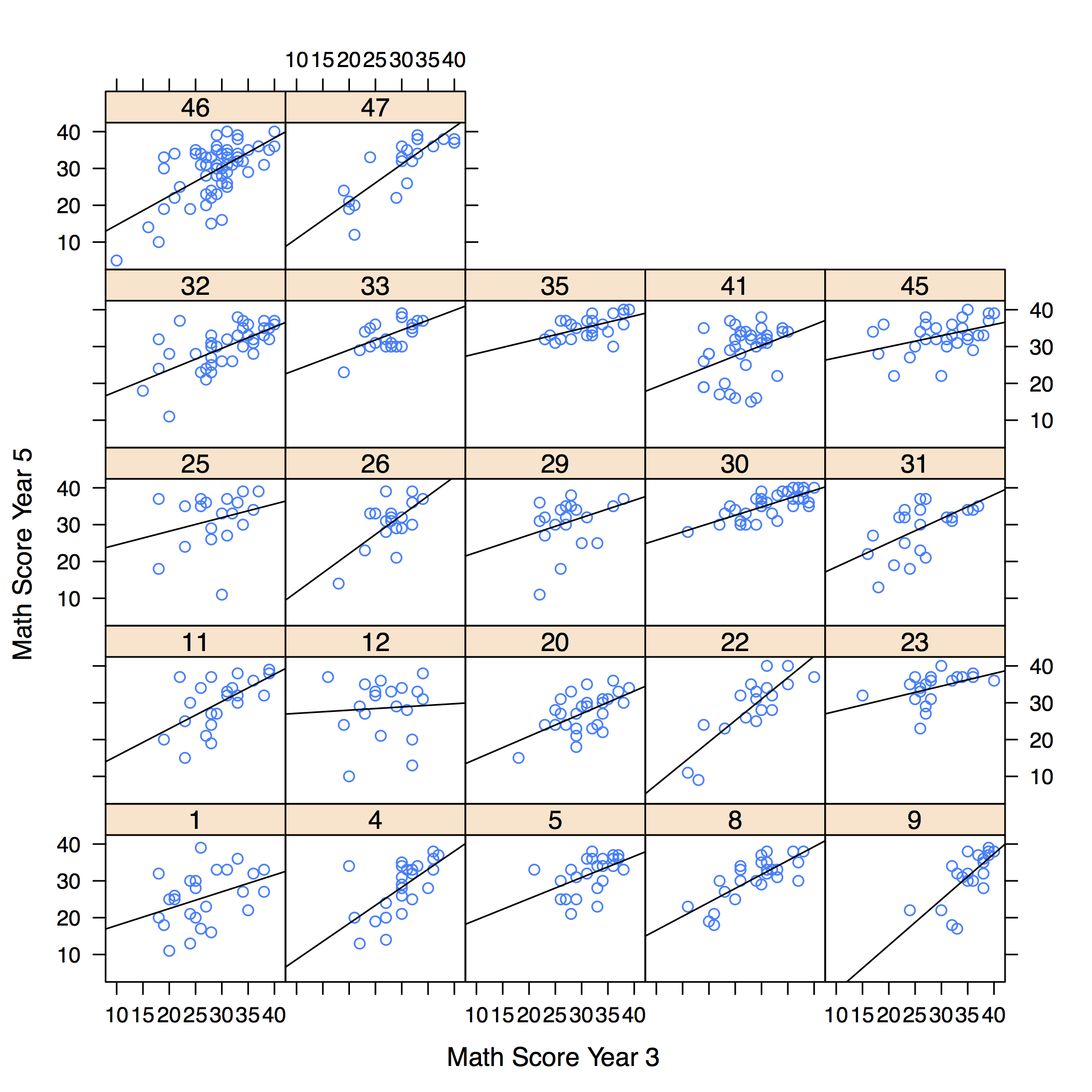
Figure 1. Scatterplots for each of the 22 schools - 4.5
- With the information obtained from the MLM, predictions might be made for every pupil in the 22 schools. For example, consider a boy student from school 32, whose previous attainment in mathematics at year 3 was 22, and whose father's occupation is classified as manual. From the MLM we know that the group-intercept for this school, û0,32 is 6.7869 and its group-slope for previous attainment û1,32 is –0.1418. These values may be incorporated into Equation 2 to obtain the predicted value in Math 5 for this student as ≈ 29.5.
An Agent-Based Model
- 5.1
- We now propose a simple ABM that addresses the problem of explaining the differences in school effectiveness by taking into account the inputs of knowledge or feedback that every pupil receives from her or his social environment in relation to one specific subject they are supposed to learn. Thus, the model considers the relevant social ties in which the pupil is embedded. To establish comparisons between this ABM and the MLM already described, we calibrate the former empirically using the same dataset . The ABM was built in NetLogo 4.1.2 (Wilensky 2011).
A mechanism-based explanation
- 5.2
- Although the literature does not provide any canonical mechanism, an important starting point is to recognise the importance of the social ties in which a pupil is embedded and its effect on her or his educational attainment. It can be assumed that the school structures the opportunities for closer friendship ties, which in turn affect peer outcomes. Since it has been demonstrated that pupils' characteristics within the classroom (such as socio-economic status and educational achievement) have an impact on the achievement of their peers (Beckerman & Good 1981; Hanushek et al. 2003), it is likely that the pupils' friendship networks are playing an important role as a mediating factor. Individuals' actions are often influenced by the people they interact with and, especially, by the actions of significant others, such as friends (Bearman et al. 2004; Kandel 1978). There is no reason to rule out, a priori, the hypothesis that a similar mechanism might produce a peer effect in educational achievement (Jæger 2007).
- 5.3
- There is a growing interest in the literature in using network topologies and friendship ties instead of school-grade cohorts as the relevant peer group (e.g., Calvó-Armengol et al. 2009; Weinberg 2007). Halliday and Kwak (2012) recently estimated peer effects using a mix of empirical data on friendship ties and school-grade cohorts. Their results suggest that the behaviour observed at the school-grade level is essentially a reduced-form approximation of a two-step process in which students first sort themselves into peer groups and then behave in a way that determines educational achievement. Although the exact sorting mechanism is not addressed in their research, it can be assumed that pupils choose their friends by a combination of contextual opportunities, geographical proximity (within the school or classroom) and 'homophily' (McPherson et al. 2001), that is, the tendency of students to group themselves with others similar to them in gender, occupational class and educational performance. Blansky and colleagues have applied this understanding to analyse how pupils' social network positions correlate with their academic achievement over time (2013). They found that students whose friends' average marks was greater (or less) than their own had a higher tendency toward increasing (or decreasing) their academic ranking over time, indicating social contagion of academic success taking place in their social network. Neal and colleagues (2013) examined classroom friendships in five U.S. elementary schools and studied self-reported (i.e., "real") and peer-reported (i.e., "inferred") relationships. They found that relationships were more likely to exist, and more likely to be inferred to exist by peers, between pairs of children who were the same sex, sat near one another, shared a positive academic orientation, or shared athletic ability. They also found that children overestimate the importance of gender in their inferences about relationships. However, gender still plays a role in the ties they form with others: children were nine times more likely to be friends if they were the same gender.
- 5.4
- Ever since the observational study carried out by Rist (2000) in the 1970s, educational researchers have been aware of the impact student-teacher relationships have on pupils' learning. Schools where teachers have higher expectations regarding the future of their students perform better than others where teachers have lower expectations (de Vos 1995). These expectations, identified as 'teacher expectations bias' or 'false-positive teacher expectations' (Jussim & Harber 2005), determine which pupils are defined as 'fast learners' and which ones as 'slow learners'. In this way, teachers' behaviour contributes to a 'self-fulfilling prophecy' (Merton 1968), that is, pupils who are considered 'slow learners' in advance receive less attention and educational feedback, and consequently, they perform worse compared to pupils who are considered 'fast learners'. Empirical research has corroborated this teacher expectation bias effect (Rosenthal & Jacobson 1968). Recently, Boer and colleagues (2010), using MLM, found a relationship between teacher expectation bias and students' characteristics as well as a clear effect of these expectations on long-term student performance. Although the evidence is still inconclusive, particularly about the magnitude of this effect and whether it accumulates or dissipates over time, it suggests that powerful self-fulfilling prophecies may occur in the classroom, and they may selectively be directed towards students from stigmatised social groups and low-achieving students.
- 5.5
- The proposed ABM presented in this paper takes into account the two mechanisms described above as the model's microspecification (Epstein 1999). That is, the model assumes that a combination of friendship dynamics based on homophily and self-fulfilling prophecy based on teacher expectations bias can produce differential achievement among students and schools. This explanatory mechanism can be established as follows. Firstly, there is a peer effect among pupils, brought about by the pupils' tendency to sort themselves into groups with similar others. This lateral group formation mechanism affects their individual learning and progress, producing groupings of pupils with different academic performances. Secondly, the differences among groups determine the way in which teachers interact with their pupils, since groups of high-performance pupils capture more attention and receive more feedback from teachers compared to groups of low-performance pupils. This vertical behavioural mechanism also affects the pupils' academic performance. This explanatory mechanism is proposed as a likely one, and additional research is needed to confirm or falsify it in real world settings.
Model description
- 5.6
- The mechanisms described above were implemented in an ABM. To build this model, we refined Wilensky's "Netlogo Party Model" (1997) to replicate the group formation mechanism. Students form groups with others similar to them following group formation rules present at the school level. For simplicity, we assume that these rules are stable and similar for all the individuals within the school (Akerlof & Kranton 2002). We are not interested in giving an account of the emergence of these rules; we take for granted they exist. We also assume for simplicity that teachers always discriminate between 'slow learner' and 'fast learner' groups, and give the corresponding feedback to the students in those groups.
- 5.7
- The ABM was designed following two basic assumptions. The first concerns the way in which pupils' group themselves. To simulate how students sort themselves into peer groups, an initial number of spots where students can 'hang out' is defined. Every school has three tolerance criteria, which are adopted by the students to decide whether to stay in a specific group or to move to the another one. Taking into account the available data, we defined three tolerance levels: Educational tolerance, which reflects the students' tolerance of accepting others with different attainments in Math 3; Gender tolerance, which indicates the students' tolerance for people of the opposite sex; and Occupational class tolerance, the pupils' tolerance for peers of a different occupational class. Each pupil is endowed with these three tolerance levels, which are identical for all the pupils within a school, but differ between schools. Tolerance levels range between 0 and 1.
- 5.8
- Pupils who belong to the same spot establish a group. If they are in a group that has, for example, a higher percentage of people of the opposite sex than the school's tolerance, then they are considered 'uncomfortable', and they leave that group for the next spot. Movement continues until everyone at the school is 'comfortable' with their group. This may result in some spots becoming empty.
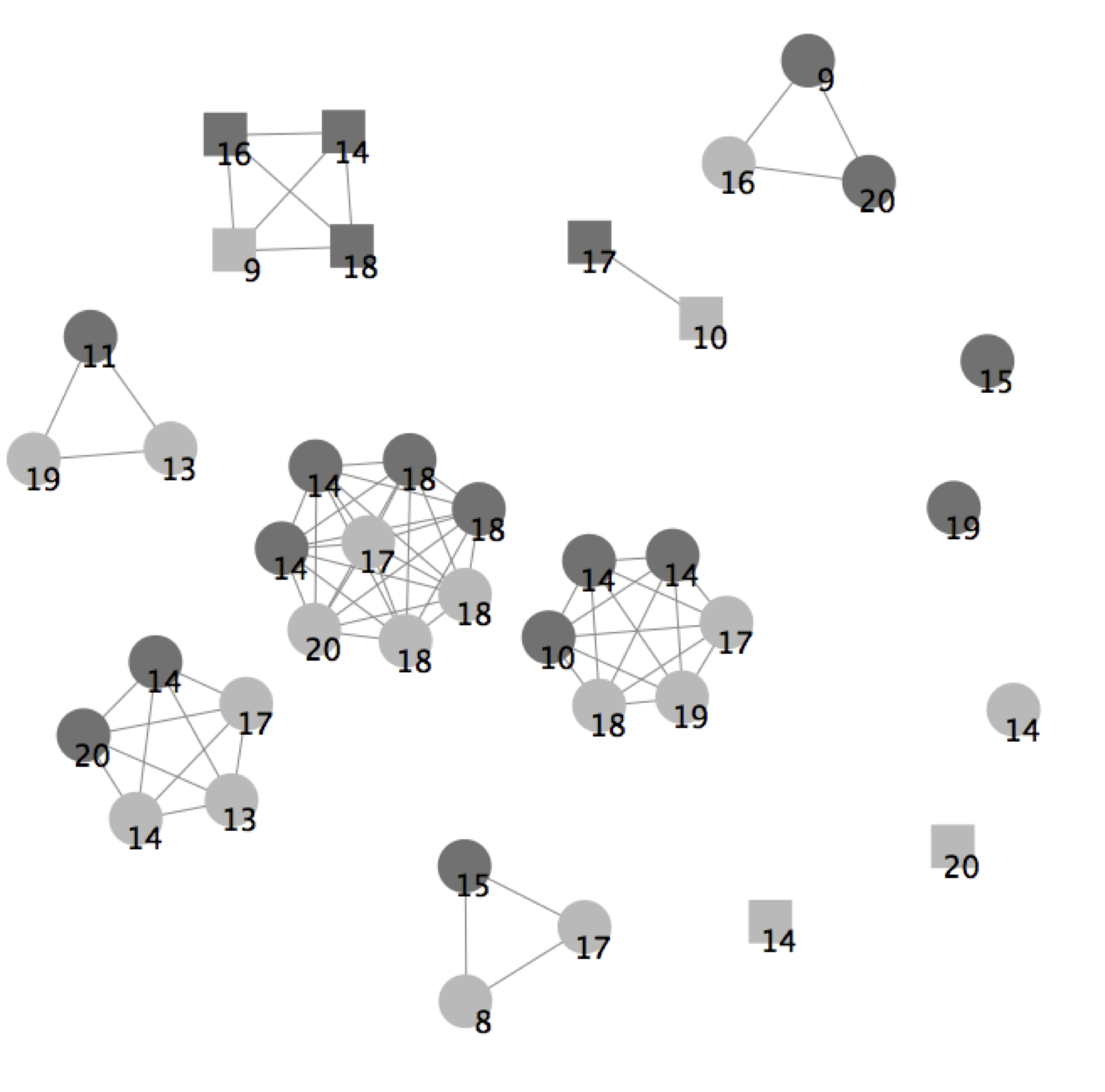
Figure 2. Simulated Students' Social Network in School #32. Boys and girls are coloured dark grey and light grey respectively; round and square shaped nodes represent low and high occupational class respectively; and the numbers show the students' previous attainment in Math 3. - 5.9
- Figure 2 shows an example of the result of this process: the student network at the end of a simulation for school 32. Male and female pupils are coloured dark grey and light grey respectively; round and square shaped nodes represent low and high occupational class respectively; and the numbers indicate their previous attainment in Math 3. In this scenario, education, gender and class tolerances are 0.9, 0.3 and 0.9 respectively. There are 39 students in school 32 and these sort themselves into 15 groups of 'friends'.
- 5.10
- The second assumption concerns the way in which pupils' learning of one specific subject evolves over time. It seems reasonable to assume that this learning can be modelled as a logarithmic function of the educational feedback received on the subject. Thus, there is an initial period of rapid increase, followed by a period where the growth in learning slows (evidence supporting this pattern of learning may be found in Baloff 1971).
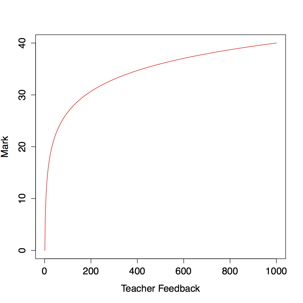
Figure 3. Simulated pupils' learning curve (defined as log(xw), where w ≈ 5.790593), which relates the teacher's feedback that the students receive and the mark or score they obtain in their tests - 5.11
- To model pupils' learning in maths from year 3 to year 5, we define a student learning curve. Firstly, we assume that learning maths is a continuous process in which the student receives feedback on the subject from the teacher. This learning process starts at the first maths lesson, lesson 0, and finishes when the knowledge of maths is measured in year 5 (or Math 5). Because we do not have any measure of the educational feedback involved in this process, we arbitrarily define 1,000 as the amount of feedback that the entire learning process involves (see Figure 3). Students' marks are assumed to be a function of the amount of teachers' feedback that they have received. We also assume that when the test Math 3 is applied, students have learned half of the topics they were supposed to learn. Further, since both Math 3 and Math 5 range between 0 and 40, we transform Math 3 by dividing it by 2.
- 5.12
- Secondly, we assume that the feedback that students receive from their teachers depends on the sorting process that pupils perform within their schools. That is, in this simulation teachers' feedback is a function of the pupils' group average achievement. Teachers use this average group achievement as a signal about the future performance of all the pupils in the group. Teachers then adjust the amount of effort they invest in educational feedback accordingly.
- 5.13
- Let gk be a group in school j, sik a student in the group and math3k the average of Math 3 marks of group gk. The amount of feedback that the students in group k receive is:
tk = (e2×math3k)1/w (3) where w in the exponent allows us to fit a logarithmic function that maps 'Teacher Feedback' into 'Mark' (see Figure 3). Since we want to fit a logarithmic function, we define w ≈ 5.790593; for we know that log(1,000w) ≈ 40, which is the scale of the test scores. Then, the simulated student's score simMath5ik is shown in Equation 4, where tik = tk+tmath3,ik and tmath3,ik is the amount of feedback the pupils in group k have had when their attainment is measured as Math 3.
simMath5ik = log (tikw) (4) - 5.14
- The following is a pseudo-code description for the model's main simulation loops:
//Setup
SET total_number_of_group_sites TO integer
INIT agents
FOR all agents
	SET agent's group_site TO integer between 1 and total_number_of_group_sites at random
ENDFOR

FOR all agents
	SET agent's is_comfortable TO boolean value
ENDFOR


//Group formation mechanism
WHILE all_agents_are_comfortable
	FOR all agents
		IF NOT agent's is_comfortable THEN
			SET agent's group_site TO an integer between 1 and total_number_of_group_sites at random
		ENDIF
	ENDFOR
	SET all_agents_are_comfortable TO Boolean value
END WHILE

//Work out math 5 marks
FOR all non empty group sites
	SET agents_in_group TO a subset of agents
	SET teacher_feedback(agents_in_group) TO a real number between 1 and 1000
	FOR agents_in_group
		SET agent's math5_mark(teacher_feedback) TO a real number
	ENDFOR
ENDFOR
Model Calibration
- 5.15
- The ABM was initialised with the pupils' performance in Math 3 and the parameter space given by the three tolerance levels was explored. The objective was to find a set of tolerance levels for each school that minimises the differences between the data and the simulation results. Let dj be such a difference for school j. Then,
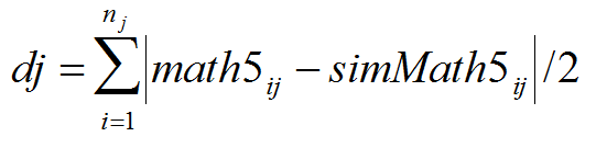
(5) where math5i and simMath5i are the score in Math 5 of student i obtained from the data and from the simulations respectively. In the example shown in Figure 2, d32 = 2.231, which means that the simulated score in Math 5 differs, on average, from the data by ±2.231 units. To explore the parameter space of the model, we ran 126,720 simulations. This represents all combinations of the three tolerances, (varying among 0.3, 0.5, 0.7 and 0.9) and the number of spots (varying among 15, 20 and 25) across the 22 schools. To have more robust results, we ran each setting 30 times and then took the average of dj over all 22 schools as the aggregate outcome.
Comparing MLM and ABM
- 6.1
- Table 3 shows the results for the parameter setting that minimises dj. We present the average distance (in the same units as the data) between the predicted scores and the real scores in Math 5 for both the multilevel model ('MLM (dj)') and the simulation ('ABM (dj)'). The table also shows the number of groups ('Final Groups') in which all the pupils were happy with their group membership, given the values in the 'Tolerance Levels' for education, gender and occupational class (the last three columns of Table 3). Recall that these three last variables were set as simulation parameters, and the specific values presented in the table correspond to those combinations at the school level that minimise the distance between the simulated and the data scores in Math 5.
Table 3: Calibration Results Tolerance Levels School Id Num. Pupils MLM (dj) ABM (dj) Final Num. of Groups Edu. Gender Occ. Class 1 25 2.88 3.36 13 0.90 0.50 0.30 4 24 2.26 3.12 12 0.90 0.90 0.50 5 25 1.53 2.26 12 0.90 0.70 0.90 8 26 1.41 2.82 12 0.90 0.70 0.30 9 21 1.67 2.91 12 0.90 0.70 0.30 11 22 1.21 3.10 12 0.90 0.30 0.70 12 19 3.03 3.55 12 0.90 0.50 0.30 20 28 1.60 2.62 12 0.90 0.30 0.70 22 18 2.18 3.63 10 0.90 0.30 0.70 23 21 1.43 3.19 12 0.90 0.90 0.50 25 20 2.60 3.50 11 0.90 0.30 0.50 26 19 1.85 2.79 12 0.90 0.70 0.50 29 20 2.30 3.36 12 0.90 0.70 0.30 30 35 1.03 2.56 14 0.70 0.90 0.70 31 22 2.30 3.60 12 0.90 0.70 0.50 32 39 1.72 2.71 15 0.90 0.30 0.90 33 25 1.22 3.04 12 0.90 0.30 0.90 35 27 1.01 2.44 13 0.90 0.70 0.30 41 38 2.46 3.25 16 0.90 0.30 0.70 45 30 1.58 2.62 12 0.90 0.30 0.70 46 62 2.24 2.96 15 0.90 0.90 0.70 47 22 1.85 3.61 12 0.90 0.50 0.90 - 6.2
- Comparing the average dj between the two models, we see that the predictions of the multilevel model (average: 1.88) outperform the predictions of the agent-based model (average 3.04), so the former is more accurate. However, the prediction errors of the ABM are not high; 3.04 on a 40 point scale is only 8%. Thus, the ABM, despite its simplicity, offers a reasonable fit to the data.
- 6.3
- The simulation results suggest a high educational tolerance, since all but one of the values is 0.9. On the other hand, the tolerance levels of occupational class and gender vary across the schools. Therefore, the group formation mechanism in the simulation seems to be ruled by the variables occupational class and gender, while previous attainment in maths does not discriminate much between groups.
- 6.4
- The hypothesised mechanism that brings about the differences in school effectiveness seems to be justified. The simulation results indicate that the mechanism of group formation helps to minimise the distance between the predicted and the actual scores, allowing a better fit with the data. For instance, comparing the number of groups with the number of pupils, in general there are fewer groups than students in each school (for a graphical example, see Figure 2). If the numbers of groups made no difference in the simulation, then the number of groups and the number of pupils would tend to be similar, at least in those schools with 25 or fewer pupils, which is the maximum number of groups the ABM calibration allowed. This is clearly not the case. In fact, for those schools with less than 25 pupils, the only variable that was significantly correlated with the model results "ABM (dj)" was the percentage of students whose fathers had non-manual jobs (r = -0.591, p = 0.026, two-tailed test), while the percentage of students at the school who were boys was not significantly correlated with the ABM performance (r = -0.062, p = 0.832, two-tailed test). The finding that class, but not gender, is important echoes the result from the MLM analysis. To sum up, the sorting mechanism that has been implemented in this simulation and the groups emerging from that mechanism seem to be important in explaining the differences in effectiveness among schools.
Concluding Remarks
- 7.1
- In this paper we have presented and compared the results of two models to address differential school effectiveness. The first was a MLM, where the hierarchical nature of educational processes is considered. The fitted model, controlling for some pupil background characteristics, was able to identify significant differences in the effectiveness of schools. However, with the available longitudinal data, it is not possible to model likely causal influences that might explain these differences. As we discussed, this is a common problem in multilevel modelling, in which, because of practical and conceptual problems, causal mechanisms are typically ignored. By building a simple ABM, we have tried to complement the statistical findings with a mechanism-based explanation. Because of the lack of a canonical mechanism-based explanation describing why school performance differences might emerge, we proposed a simple one, based not on direct empirical data but on plausible dynamics that previous research has found likely to explain differences in academic performance among pupils. These social mechanisms referred to the effects of friendship ties and teacher expectations bias on pupils' educational achievement. They were the ABM micro-specification.
- 7.2
- We found that the MLM provides more accurate predictions than the ABM. However, although the ABM is rather simple, the differences in the magnitude of the prediction errors are small. The analyses from the two models made clear that, whereas MLM is data driven, ABM is both data driven and theory based, so the latter allows researchers to formalise and falsify in silico plausible mechanisms that might bring about the observed differences in performance across schools. In short, although the fitted MLM outperforms the proposed ABM, the latter still offers a reasonable fit and provides a causal mechanism to explain differences in the identified school performances that is absent in the MLM.
- 7.3
- The next research step might be to falsify the proposed mechanism in 'real world settings'. This would help to interpret and explain the differences established using MLM. That is, for researchers to determine whether friendship ties and teacher expectation bias provide an adequate explanation of differential school effectiveness, as we have computationally demonstrated here, one needs to gauge the results with peer effects and teacher expectations estimates based on actual (and not simulated) peer networks. This paper has stressed that both the generative sufficiency of ABM and the inferential nature of MLM can be complemented to provide sociological research with more powerful tools. Our work presents a first step in this direction.
Acknowledgements
-
This paper is based on research carried out as part of an Economic and Social Research Council National Centre for Research Methods Collaborative Project on 'Multilevel and Agent-Based Modelling: Comparison and Integration'. We thank Edmund Chattoe-Brown, Fiona A. Steele, Sylvia Richardson and the referees for their comments on earlier versions of this paper. Dr. Salgado also thanks the support received by the 'Attraction and Insertion of Advanced Human Capital Program', through its funding instrument 'Support for the Return of Researchers from Abroad 2012', of the National Commission for Scientific and Technological Research of Chile (CONICYT-PAI 82130019).
Notes
-
1To corroborate the robustness of this analysis, we estimated the three models on the entire sample. The results confirmed that Model 3 had the best overall fit, significantly better than either of the other two
References
-
AKERLOF, G. A., & Kranton, R. E. (2002). Identity and Schooling: Some Lessons for the Economics of Education. Journal of Economic Literature, 40(4), 1167–1201. [doi:10.1257/.40.4.1167]
BALOFF, N. (1971). Extension of the Learning Curve - Some Empirical Results. Operational Research Quarterly (1970–1977), 22(4), 329–340. [doi:10.2307/3008186]
BEARMAN, P. S., Moody, J., & Stovel, K. (2004). Chains of Affection: The Structure of Adolescent Romantic and Sexual Networks. The American Journal of Sociology, 110(1), 44–91. [doi:10.1086/386272]
BECKERMAN, T. M., & Good, T. L. (1981). The Classroom Ratio of High- and Low-Aptitude Students and Its Effect on Achievement. American Educational Research Journal, 18(3), 317–327. [doi:10.3102/00028312018003317]
BEHRMAN, J. R., & Rosenzweig, M. R. (2002). Does Increasing Women's Schooling Raise the Schooling of the Next Generation? The American Economic Review, 92(1), 323–334. [doi:10.1257/000282802760015757]
BLANSKY, D., Kavanaugh, C., Boothroyd, C., Benson, B., Gallagher, J., Endress, J., & Sayama, H. (2013). Spread of Academic Success in a High School Social Network. PLoS ONE, 8(2), e55944. [doi:10.1371/journal.pone.0055944]
BLIESE, P. D. (2000). Within-group agreement, non-independence, and reliability: Implications for data aggregation and analysis. In K. J. Klein & S. W. J. Kozlowski (Eds.), Multilevel theory, research, and methods in organizations: Foundations, extensions, and new directions (pp. 349–381). San Francisco: Jossey-Bass.
CALVÓ-ARMENGOL, A., Patacchini, E., & Zenou, Y. (2009). Peer Effects and Social Networks in Education. Review of Economic Studies, 76(4), 1239–1267. [doi:10.1111/j.1467-937X.2009.00550.x]
CARRINGTON, P. J., Scott, J., & Wasserman, S. (Eds.). (2005). Models and methods in social network analysis. New York: Cambridge University Press. [doi:10.1017/CBO9780511811395]
CEDERMAN, L.E. (2005). Computational Models of Social Forms: Advancing Generative Process Theory. American Journal of Sociology, 110(4), 864–893. [doi:10.1086/426412]
COLEMAN, J. S. (1966). Equality of Educational Opportunity Study (EEOS). Washington: National Center for Educational Statistics. Retrieved from http://www.eric.ed.gov/ERICWebPortal/contentdelivery/servlet/ERICServlet?accno=ED012275
DE BOER, H., Bosker, R. J., & van der Werf, M. P. C. (2010). Sustainability of teacher expectation bias effects on long-term student performance. Journal of Educational Psychology, 102(1), 168–179. [doi:10.1037/a0017289]
DE VOS, H. (1995). Using Simulation To Study School Effectiveness. Presented at the The Annual Meeting of the European Council on Educational Research, Bath, England. Retrieved from http://www.eric.ed.gov/ERICWebPortal/contentdelivery/servlet/ERICServlet?accno=ED396369
EPPLE, D., & Romano, R. E. (1998). Competition between Private and Public Schools, Vouchers, and Peer-Group Effects. The American Economic Review, 88(1), 33–62.
EPSTEIN, J. M. (1999). Agent-based computational models and generative social science. Complexity, 4(5), 41–60. [doi:10.1002/(SICI)1099-0526(199905/06)4:5<41::AID-CPLX9>3.0.CO;2-F]
EVANS, W. N., Oates, W. E., & Schwab, R. M. (1992). Measuring Peer Group Effects: A Study of Teenage Behavior. Journal of Political Economy, 100(5), 966–991. [doi:10.1086/261848]
GELMAN, A., & Hill, J. (2006). Data Analysis Using Regression and Multilevel/Hierarchical Models (1st ed.). Cambridge University Press. [doi:10.1017/CBO9780511790942]
GILBERT, N. (2008). Agent-Based Models. California: Sage Publications Ltd.
GODDARD, R. D., & Goddard, Y. L. (2001). A multilevel analysis of the relationship between teacher and collective efficacy in urban schools. Teaching and Teacher Education, 17(7), 807–818. [doi:10.1016/S0742-051X(01)00032-4]
GOLDSTEIN, H., Burgess, S., & McConnell, B. (2007). Modelling the effect of pupil mobility on school differences in educational achievement. Journal of the Royal Statistical Society: Series A (Statistics in Society), 170(4), 941–954. [doi:10.1111/j.1467-985X.2007.00491.x]
HALLIDAY, T. J., & Kwak, S. (2012). What is a peer? The role of network definitions in estimation of endogenous peer effects. Applied Economics, 44, 289–302. [doi:10.1080/00036846.2010.505557]
HANUSHEK, E. A., Kain, J. F., Markman, J. M., & Rivkin, S. G. (2003). Does peer ability affect student achievement? Journal of Applied Econometrics, 18(5), 527–544. [doi:10.1002/jae.741]
HANUSHEK, E. A., & Taylor, L. L. (1990). Alternative Assessments of the Performance of Schools: Measurement of State Variations in Achievement. The Journal of Human Resources, 25(2), 179–201. [doi:10.2307/145753]
HARKER, R., & Tymms, P. (2004). The Effects of Student Composition on School Outcomes. School Effectiveness and School Improvement, 15(2), 177–199. [doi:10.1076/sesi.15.2.177.30432]
HEDSTRÖM, P. (2005). Dissecting the Social: On the Principles of Analytical Sociology. Cambridge: Cambridge University Press. [doi:10.1017/CBO9780511488801]
HEDSTRÖM, P., & Swedberg, R. (1996). Social Mechanisms. Acta Sociologica, 39(3), 281–308. [doi:10.1177/000169939603900302]
JÆGER, M. M. (2007). Economic and Social Returns To Educational Choices. Rationality and Society, 19(4), 451–483. [doi:10.1177/1043463107083739]
JUSSIM, L., & Harber, K. D. (2005). Teacher Expectations and Self-Fulfilling Prophecies: Knowns and Unknowns, Resolved and Unresolved Controversies. Personality and Social Psychology Review, 9(2), 131–155. [doi:10.1207/s15327957pspr0902_3]
KANDEL, D. B. (1978). Homophily, Selection, and Socialization in Adolescent Friendships. The American Journal of Sociology, 84(2), 427–436. [doi:10.1086/226792]
LADD, H. F., & Walsh, R. P. (2002). Implementing value-added measures of school effectiveness: getting the incentives right. Economics of Education Review, 21(1), 1–17. [doi:10.1016/S0272-7757(00)00039-X]
LAZEAR, E. P. (2001). Educational Production. The Quarterly Journal of Economics, 116(3), 777–803. [doi:10.1162/00335530152466232]
LECKIE, G. (2009). The complexity of school and neighbourhood effects and movements of pupils on school differences in models of educational achievement. Journal of the Royal Statistical Society: Series A (Statistics in Society), 172(3), 537–554. [doi:10.1111/j.1467-985X.2008.00577.x]
LEE, V. E., & Bryk, A. S. (1989). A Multilevel Model of the Social Distribution of High School Achievement. Sociology of Education, 62(3), 172–192. [doi:10.2307/2112866]
MACY, M. W., & Willer, R. (2002). From factors to actors: Computational Sociology and Agent-Based Modeling. Annual Review of Sociology, 28(1), 143–166. [doi:10.1146/annurev.soc.28.110601.141117]
MAROULIS, S., Bakshy, E., Gomez, L., & Wilensky, U. (2010a). An agent-based model of intra-district public choice. Retrieved from http://ccl.northwestern.edu/papers/choice.pdf
MAROULIS, S., Guimerà, R., Petry, H., Stringer, M. J., Gomez, L. M., Amaral, L. a. N., & Wilensky, U. (2010b). Complex Systems View of Educational Policy Research. Science, 330(6000), 38–39. [doi:10.1126/science.1195153]
MANSKI, C. F. (1993). Identification of Endogenous Social Effects: The Reflection Problem. The Review of Economic Studies, 60(3), 531–542. [doi:10.2307/2298123]
MANZO, G. (2007). Variables, Mechanisms, and Simulations: Can the Three Methods Be Synthesized? Revue Française de Sociologie, 48(5), 35–71. [doi:10.3917/rfs.485.0035]
MANZO, G. (2013). Educational Choices and Social Interactions: A Formal Model and a Computational Test. In G. E. Birkelund (Ed.), Comparative Social Research (Vol. 30, pp. 47–100). Emerald Group Publishing Limited. [doi:10.1108/s0195-6310(2013)0000030007]
MCPHERSON, M., Smith-Lovin, L., & Cook, J. M. (2001). Birds of a Feather: Homophily in Social Networks. Annual Review of Sociology, 27(1), 415–444. [doi:10.1146/annurev.soc.27.1.415]
MERTON, R. K. (1968). Social Theory and Social Structure. New York: Free Press.
MEYER, R.H. (1997). Value-added indicators of school performance: A primer. Economics of Education Review, 16(3), 283–301. [doi:10.1016/S0272-7757(96)00081-7]
MONTES, G. (2011). Using Artificial Societies to Understand the Impact of Teacher Student Match on Academic Performance: The Case of Same Race Effects. Journal of Artificial Societies and Social Simulation, 15(4), 8.
NEAL, J. W., Neal, Z. P., & Cappella, E. (2013). I Know Who My Friends Are, but Do You? Predictors of Self-Reported and Peer-Inferred Relationships. Child Development, [Forthcoming].
NUTTALL, D. L., Goldstein, H., Prosser, R., & Rasbash, J. (1989). Differential school effectiveness. International Journal of Educational Research, 13(7), 769–776. [doi:10.1016/0883-0355(89)90027-X]
PATERSON, L., & Goldstein, H. (1991). New Statistical Methods for Analysing Social Structures: an introduction to multilevel models. British Educational Research Journal, 17(4), 387–393. [doi:10.1080/0141192910170408]
PINHEIRO, J. C., & Bates, D. M. (1996). Unconstrained Parameterizations for Variance-Covariance Matrices. Statistics and Computing, 6, 289–296. [doi:10.1007/BF00140873]
R DEVELOPMENT CORE TEAM. (2013). R: A language and environment for statistical computing. Vienna, Austria. Retrieved from http://www.R-project.org
REYNOLDS, D., Chapman, C., Kelly, A., Muijs, D., & Sammons, P. (2011). Educational effectiveness: the development of the discipline, the critiques, the defence, and the present debate. Effective Education, 3(2), 109–127. [doi:10.1080/19415532.2011.686168]
RIST, R. (2000). Student Social Class and Teacher Expectations: The Self-Fulfilling Prophecy in Ghetto Education. Harvard Educational Review, 70(3), 257–302. [doi:10.17763/haer.70.3.1k0624l6102u2725]
ROSENTHAL, R., & Jacobson, L. (1968). Pygmalion in the Classroom: Teacher Expectation and Pupils' Intellectual Development (First Printing.). New York: Holt, Rinehart & Winston.
SAMMONS, P., Nuttall, D., & Cuttance, P. (1993). Differential School Effectiveness: Results from a Reanalysis of the Inner London Education Authority's Junior School Project Data. British Educational Research Journal, 19(4), 381–405. [doi:10.1080/0141192930190407]
SINGER, J. D. (1998). Using SAS PROC MIXED to Fit Multilevel Models, Hierarchical Models, and Individual Growth Models. Journal of Educational and Behavioral Statistics, 23(4), 323–355. [doi:10.2307/1165280]
STEELE, F., Vignoles, A., & Jenkins, A. (2007). The effect of school resources on pupil attainment: a multilevel simultaneous equation modelling approach. Journal of the Royal Statistical Society: Series A (Statistics in Society), 170(3), 801–824. [doi:10.1111/j.1467-985X.2007.00476.x]
STOICA, V. I., & Flache, A. (2014). From Schelling to Schools: A Comparison of a Model of Residential Segregation with a Model of School Segregation. Journal of Artificial Societies and Social Simulation, 17(1), 5.
WEINBERG, B. A. (2007). Social Interactions with Endogenous Associations. National Bureau of Economic Research Working Paper Series, No. 13038. Retrieved from http://www.nber.org/papers/w13038
WILENSKY, U. (1997). NetLogo Party model. Evanston, IL.: Center for Connected Learning and Computer-Based Modeling, Northwestern University. Retrieved from http://ccl.northwestern.edu/netlogo/models/Party
WILENSKY, U. (2011). NetLogo. Center for Connected Learning and Computer-Based Modeling. Northwestern University, Evanston, IL. Retrieved from http://ccl.northwestern.edu/netlogo
WU, H.C., & Sun, C.T. (2005). What Should We Do Before Running a Social Simulation?: The Importance of Model Analysis. Social Science Computer Review, 23(2), 221–234. [doi:10.1177/0894439304273270]