
 Abstract
- Agent-based models are increasingly used to address questions regarding real-world phenomena and mechanisms; therefore, the calibration of model parameters to certain data sets and patterns is often needed. Furthermore, sensitivity analysis is an important part of the development and analysis of any simulation model. By exploring the sensitivity of model output to changes in parameters, we learn about the relative importance of the various mechanisms represented in the model and how robust the model output is to parameter uncertainty. These insights foster the understanding of models and their use for theory development and applications. Both steps of the model development cycle require massive repetitions of simulation runs with varying parameter values. To facilitate parameter estimation and sensitivity analysis for agent-based modellers, we show how to use a suite of important established methods. Because NetLogo and R are widely used in agent-based modelling and for statistical analyses, we use a simple model implemented in NetLogo as an example, packages in R that implement the respective methods, and the RNetLogo package, which links R and NetLogo. We briefly introduce each method and provide references for further reading. We then list the packages in R that may be used for implementing the methods, provide short code examples demonstrating how the methods can be applied in R, and present and discuss the corresponding outputs. The Supplementary Material includes full, adaptable code samples for using the presented methods with R and NetLogo. Our overall aim is to make agent-based modellers aware of existing methods and tools for parameter estimation and sensitivity analysis and to provide accessible tools for using these methods. In this way, we hope to contribute to establishing an advanced culture of relating agent-based models to data and patterns observed in real systems and to foster rigorous and structured analyses of agent-based models.
- Keywords:
- Parameter Fitting, Sensitivity Analysis, Model Calibration, Agent-Based Model, Inverse Modeling, NetLogo
Introduction
- 1.1
- In agent-based models (ABMs), individual agents, which can be humans, institutions, or organisms, and their behaviours are represented explicitly. ABMs are used when one or more of the following individual-level aspects are considered important for explaining system-level behaviour: heterogeneity among individuals, local interactions, and adaptive behaviour based on decision making (Grimm 2008). The use of ABMs is thus required for many, if not most, questions regarding social, ecological, or any other systems comprised of autonomous agents. ABMs have therefore become an established tool in social, ecological and environmental sciences (Gilbert 2007; Thiele et al. 2011; Railsback & Grimm 2012).
- 1.2
- This establishment appears to have occurred in at least two phases. First, most ABMs in a certain field of research are designed and analysed more or less ad hoc, reflecting the fact that experience using this tool must accumulate over time. The focus in this phase is usually more on how to build representations than on in-depth analyses of how the model systems actually work. Typically, model evaluations are qualitative, and fitting to data is not a major issue. Most models developed in this phase are designed to demonstrate general mechanisms or provide generic insights. The price for this generality is that the models usually do not deliver testable predictions, and it remains unclear how well they really explain observed phenomena.
- 1.3
- The second phase in agent-based modelling appears to begin once a critical mass of models for certain classes of questions and systems has been developed, so that attention shifts from representation and demonstration to obtaining actual insights into how real systems are working. An indicator of this phase is the increased use of quantitative analyses that focus on both a better mechanistic understanding of the model and on relating the model to real-world phenomena and mechanisms. Important approaches during this stage are sensitivity analysis and calibration (parameter fitting) to certain data sets and patterns.
- 1.4
- The use of these approaches is, however, still rather low with agent-based modelling. A brief survey of papers published in the Journal of Artificial Societies and Social Simulation and in Ecological Modelling in the years 2009–2010 showed that the percentages of simulation studies including parameter fitting were 14 and 37%, respectively, while only 12 and 24% of the published studies included some type of systematic sensitivity analysis (for details of this survey, see Supplement SM1). There are certainly many reasons why quantitative approaches for model analysis and calibration are not used more often and why the usage of these approaches appears to differ between social simulation and ecological modelling, including the availability of data and generally accepted theories of certain processes, a focus on theory or application, and the complexity of the agents' decision making (e.g., whether they are humans or plants).
- 1.5
- There is, however, a further important impediment to using more quantitative methods for analysing models and relating them more closely to observed patterns (Grimm, Revilla, Berger, et al. 2005; Railsback & Grimm 2012) and real systems: most modellers in ecology and social sciences are amateurs with regard to computer science and the concepts and techniques of experimental design (Lorscheid et al. 2012). They often lack training in methods for calibration and sensitivity analysis and for implementing and actually using these methods. Certainly, comprehensive monographs on these methods exist (e.g., Saltelli et al. 2004; Kleijnen 2008), but they tend to be dense and therefore not easily accessible for many modellers in social sciences and ecology. Moreover, even if one learns how a certain method works in principle, it often remains unclear how it should actually be implemented and used.
- 1.6
- We therefore in this article introduce software and provide scripts that facilitate the use of a wide range of methods for calibration, the design of simulation experiments, and sensitivity analysis. We do not intend to give in-depth introductions to these methods but rather provide an overview of the most important approaches and demonstrate how they can easily be applied using existing packages for the statistical software program R (R Core Team 2013a) in conjunction with RNetLogo (Thiele et al. 2012), an R package that allows a NetLogo (Wilensky 1999) model to be run from R, sends data to that model, and exports the model output to R for visualisation and statistical analyses.
- 1.7
- R is a free, open-source software platform that has become established as a standard tool for statistical analyses in biology and other disciplines. An indicator of this is the rapidly increasing number of textbooks on R or on certain elements of R; currently, there are more than 30 textbooks on R (R Core Team 2013b) available, e.g., Crawley (2005); Dalgaard ( 2008) and Zuur et al. (2009). R is an open platform, i.e., users contribute packages that perform certain tasks. RNetLogo is one of these packages.
- 1.8
- NetLogo (Wilensky 1999) is a free software platform for agent-based modelling that was originally designed for teaching but is increasingly used for science (Railsback & Grimm 2012; Wilensky & Rand, in press). Learning and using NetLogo requires little effort due to its easy and stable installation, the excellent documentation and tutorials, a simple but powerful programming language, and continuous support by its developers and users via an active user forum on the internet. Moreover, NetLogo's source code was made available to the public in 2011, which might lead to further developments and improvements, in particular regarding computational power, which can sometimes be limiting for large, complex models.
- 1.9
- NetLogo comes with "BehaviorSpace" (Wilensky & Shargel 2002), a convenient tool for running simulation experiments, i.e., automatically varying parameters, running simulations, and writing model outputs to files. However, for more complex calibrations, simulation experiments, or sensitivity analyses, it would be more efficient to have a seamless integration of NetLogo into software where modules or packages for these complex methods exist and can easily be used and adapted. Such a seamless link has been developed for Mathematica (Bakshy & Wilensky 2007) and, more recently, also for R (RNetLogo, Thiele et al. 2012). RNetLogo merges the power of R with the power and ease of use of NetLogo.
- 1.10
- The software tool "BehaviorSearch" calibrates ABMs implemented in NetLogo (Stonedahl & Wilensky 2013); it implements some of the calibration methods that we describe below and appears to be powerful and robust (for an example use, see Radchuk et al. 2013). Still, for many purposes, the professional agent-based modeller might need to take advantage of the wider range of calibration methods available via R packages and to control the operation of these methods in more detail. We recommend using the "cookbook" presented here in combination with BehaviorSearch. For models implemented in languages other than NetLogo, the scripts in our cookbook can be adapted because they are based on R, whereas BehaviorSearch cannot be used.
- 1.11
- In the following, we will first explain how R, NetLogo, and RNetLogo are installed and how these programs can be learned. We introduce a simple example model, taken from population ecology, which will be used for all further demonstrations. We then present a wide range of techniques of model calibration, starting with a short general introduction and closing with an intermediate discussion. Afterwards, we do the same for sensitivity analysis techniques. Our main purpose is to provide an overview, or "cookbook", of methods so that beginners in parameter estimation and sensitivity analysis can see which approaches are available, what they can be used for, and how they are used in principle using R scripts. These scripts can also be adapted if platforms other than NetLogo are used for implementing the ABM, but then the users must replace the "simulation function" in the R scripts, where the data exchange between R and NetLogo occurs, with an appropriate alternative. All source codes, i.e., the NetLogo model implementation and the R/RNetLogo scripts, are available in the Supplementary Material.
- 1.12
- We will not discuss the backgrounds of the methods in detail, as there is already a large body of literature on calibration and sensitivity analysis methods (e.g., Saltelli et al. 2000, 2004, 2008; Helton et al. 2006; Kleijnen 1995, 2008; Cournède et al. 2013; Gan et al. 2014). We will therefore refer to existing introductions to the respective methods. We also did not fine-tune the methods to our example model and did not perform all of the checks required for thorough interpretation of results, e.g., convergence checks. Therefore, the methods presented have the potential to produce more detailed and robust results, but for simplicity, we used default settings whenever possible. The purpose of this article is not to present the optimal application of the methods for the example model but to provide a good starting point to apply the methods to readers' own models. As with a real cookbook, readers should benefit from reading the general sections but might decide to browse through the list of approaches demonstrated and selectively zoom into reading specific "recipes".
- 1.13
- Readers not familiar with R will not understand the R scripts in detail but can still see how easily R packages can be employed to perform even complex tasks. Readers not familiar with statistical methods, e.g., linear regression, will not understand the interpretation of some of the results presented, but they should still grasp the general idea. Again, as with a real cookbook, you will not be able to follow the recipe if you never learned the basics of cooking. However, hopefully this article will convince some readers that learning these basics might pay off handsomely.
Software requirements
- 1.14
- The model used and described in the next section is implemented in NetLogo (Wilensky 1999). NetLogo can be downloaded from http://ccl.northwestern.edu/netlogo/. Parameter fitting and sensitivity analysis is performed in R (R Core Team 2013a). R can be downloaded from http://cran.r-project.org/. Because RNetLogo is available on CRAN, installation from within an R shell/RGUI can be performed by typing install.packages("RNetLogo"). For further details see the RNetLogo manual, available at http://cran.r-project.org/web/packages/RNetLogo/index.html. When RNetLogo is installed, loading the example model works in this way (path and version names might need to be adapted):
# 1. Load the package.
library(RNetLogo)
# 2. Initialize NetLogo.
nl.path <- "C:/Program Files/Netlogo 5.0.4"
NLStart(nl.path, nl.version=5, gui=FALSE, obj.name="my.nl1")
# 3. Load the NetLogo model.
model.path <- "C:/models/woodhoopoe.nlogo"
NLLoadModel(model.path, nl.obj="my.nl1") - 1.15
- This code was used in all application examples. The source codes of all examples as well as the R workspaces with simulation results are in the Supplementary Material. In many of the examples presented in this article, additional R packages are used. In most cases the installation is equivalent to the installation of RNetLogo. References are provided where these packages are used.
The example model
- 1.16
- The model description following the ODD protocol (Grimm et al. 2010) is adopted from Railsback & Grimm (2012). Because they are simple, a description of the submodels is included in the section Process overview and scheduling. The source code of the NetLogo model is included in the Supplementary Material.
- 1.17
- The model represents, in a simplified way, the population and social group dynamics of a group-living, territorial bird species with reproductive suppression, i.e., the alpha couple in each group suppresses the reproduction of subordinate mature birds. A key behaviour in this system is the subordinate birds' decision as to when to leave their territory for so-called scouting forays, on which they might discover a free alpha, or breeding, position somewhere else. If they do not find such a position, they return to their home territory. Scouting forays come with an increased mortality risk due to raptors. The model provides a laboratory for developing a theory for the scouting foray decision, i.e., alternative submodels of the decision to foray can be implemented and the corresponding output of the full model compared to patterns observed in reality. Railsback & Grimm (2012) use patterns generated by a specific model version, and the educational task they propose is to identify the submodel they were using. In this article, we use the simplest model version, where the probability of subordinates undertaking a scouting foray is constant.
- 1.18
- Purpose. – The purpose of the model is to explore the consequences of the subordinate birds' decisions to make scouting forays on the structure and dynamics of the social group and the entire population.
- 1.19
- Entities, state variables, and scales. – The entities of the model are birds and territories. A territory represents both a social group of birds and the space occupied by that group. Territories not occupied by a group are empty. Territories are arranged in a one-dimensional row of 25 NetLogo patches with the boundary territories "wrapped" so that the model world is a ring. The state variables of a territory are the coordinate of its location and a list of the birds occupying it. The state variables of birds are their sex, age (in months), and whether they are alpha. The time step of the model is one month. Simulations run for 22 years, and the results from the initial two years are ignored.
- 1.20
- Process overview and scheduling. – The following list of processes is executed in the given order once per time step. The order in which the birds and territories execute a process is always randomised, and state variables are updated immediately after each operation.
- Date and ages of birds are updated.
- Territories try to fill vacant alpha positions. If a territory lacks an alpha but has a subordinate adult (age > 12 months) of the right sex, the oldest subordinate becomes the new alpha.
- Birds undertake scouting forays. Subordinate adults decide whether to scout for a new territory with a vacant alpha position. If no other non-alpha is in the current territory, a subordinate adult definitely stays. If there are older non-alphas on the current home territory, a subordinate adult scouts with probability scout-prob. If the bird scouts, it randomly moves either left or right along the row of territories. Scouting birds can explore up to scouting-distance territories in their chosen direction. Of those territories, the bird occupies the one that is closest to its starting territory and has no alpha of its sex. If no such territory exists, the bird goes back to its starting territory. All birds that scout (including those that find and occupy a new territory) are then subjected to a predation mortality probability of 1.0 - scouting-survival.
- Alpha females reproduce. In the last month of every year, alpha females that have an alpha male in their territory produce two offspring. The offspring have their age set to zero months and their sex chosen randomly with equal probability.
- Birds experience mortality. All birds are subject to stochastic background mortality with a monthly survival probability of survival-prob.
- Output is produced.
- 1.21
- Design concepts.
- Emergence. The results we are interested in are the three patterns the model is supposed to reproduce (see Observation); they all emerge from the decision making for scouting but also may strongly depend on other model parameters, such as reproduction and mortality rates.
- Adaptation. There is only one adaptive decision: to undertake a scouting foray or not.
- Objectives. The subordinate birds' objective is to become an alpha so they can reproduce. If the individual stays at its home territory, all the older birds of its sex must die before the individual is able to become an alpha. If the individual scouts, to succeed it must find a vacant alpha position and it must survive predation during scouting.
- Sensing. We assume that birds know nothing about other territories and can only sense whether an alpha position is open in another territory by actually going there. Birds know both the status and age of the other birds in their group.
- Collectives. The social groups are collectives. Because the model's "territory" entities represent the social groups as well as their space, the model treats the behaviours of the social groups (promoting alphas) as behaviours of the territories.
- Observation. In addition to visual displays to observe individual behaviour, three characteristic patterns are observed at different hierarchical levels of the model: the long-term mean number of birds (mean or abundance criterion), the standard deviation from year to year in the annual number of birds (variation criterion) and the average percentage of territories that lack one or both alpha animals (vacancy criterion). The observational data are collected in November of each year, i.e., the month before reproduction occurs.
- 1.22
- Initialisation. – Simulations begin in January (month 1). Every territory begins with two male and two female birds, with ages chosen randomly from a uniform distribution of 1 to 24 months. The oldest adult of each sex becomes alpha.
- 1.23
- Input data. – The model does not include any external input.
- 1.24
- Submodels. – Because all submodels are very simple, their full descriptions are already included in the process overview above.
- 1.25
- The model includes five parameters, which are listed in Table 1.
Table 1: Model parameters. Parameter Description Base value used by Railsback & Grimm (2012) fecundity Number of offspring per reproducing female 2 scouting-distance Distance over which birds scout 5 scouting-survival Probability of surviving a scouting trip 0.8 survival-prob Probability of a bird to survive one month 0.99 scout-prob Probability to undertake a scouting trip 0.5
Parameter estimation and calibration
- 2.1
- Typically, ABMs include multiple submodels with several parameters. Parameterisation, i.e., finding appropriate values of at least some of these parameters, is often difficult due to the uncertainty in, or complete lack of, observational data. In such cases, parameter fitting or calibration methods can be used to find reasonable parameter values by combining sampling or optimisation methods with so-called inverse modelling, also referred to as pattern-oriented parameterisation/modelling (POM; Grimm & Railsback 2005), or Monte Carlo Filtering, as the patterns are applied as filters to separate good from bad sets of parameter values (Grimm & Railsback 2005). The basic idea is to find parameter values that make the model reproduce patterns observed in reality sufficiently well.
- 2.2
- Usually, at least a range of possible values for a parameter is known. It can be obtained from biological constraints (e.g., an adult human will usually be between 1.5 and 2.2 metres tall), by checking the variation in repeated measurements or different data in the literature, etc. During model development, parameter values are often chosen via simple trial and error "by hand" because precision is not necessary at this stage. However, once the design of the model is fixed and more quantitative analyses are planned, the model must be run systematically with varying parameter values within this range and the outcome of the model runs compared to observational data.
- 2.3
- If the parameters are all independent, i.e., the calibrations of different parameters do not affect each other, it is possible to perform model calibration separately for all unknown parameters. Usually, though, parameters interact because the different processes that the parameters represent are not independent but interactive. Thus, rather than single parameters, entire sets of parameters must be calibrated simultaneously. The number of possible combinations can become extremely large and may therefore not be processable within adequate time horizons.
- 2.4
- Therefore, more sophisticated ways of finding the right parameter values are needed. This can also be the case for independent parameters or if only one parameter value is unknown, if the model contains stochastic effects and therefore needs to be run multiple times (Monte Carlo simulations) for each parameter combination (Martínez et al. 2011) or if the model runs very slow. Therefore, efficient sampling or optimisation methods must be applied. Here, "sampling" refers to defining parameter sets so that the entire parameter space, i.e., all possible parameter combinations, is explored in a systematic way.
- 2.5
- To assess whether a certain combination of parameter values leads to acceptable model output, it is necessary to define one, or better yet multiple, fitting criteria, i.e., metrics that allow one to quantify how well the model output matches the data. Such criteria should be taken from various hierarchical levels and possibly different spatial or temporal scales, e.g., from single individuals over social groups, if possible, to the whole population.
- 2.6
- Two different strategies for fitting model parameters to observational data exist: best-fit and categorical calibration. The aim of calibration for the first strategy is to find the parameter combination that best fits the observational data. The quality measure is one exact value obtained from the observational data, so it is easy to determine which parameter set leads to the lowest difference. Of course, multiple fitting criteria can be defined, but they must be aggregated to one single measure, for example, by calculating the sum of the mean square deviation between the model and the observational data for all fitting criteria. An example for the application of such a measure can be found in Wiegand et al. (1998). The problem with best-fit calibration is that even the best parameter set may not be able to reproduce all observed patterns sufficiently well. Furthermore, aggregating different fitting criteria to one measure makes it necessary to think about their relation to each other, i.e., are they all equally important or do they need to be weighted?
- 2.7
- These questions are not that important for the second strategy, categorical calibration. Here, a single value is not derived from the observational data, but rather, a range of plausible values is defined for each calibration criterion. This is particularly useful when the observational data are highly variable or uncertain by themselves. In this case, the number of criteria met is counted for a parameter set, i.e., the cases when the model result matches the defined value range. Then, the parameter set that matches all or most criteria is selected. Still, it is possible that either no parameter combination will match the defined value range or that multiple parameter sets will reproduce the same target patterns. In such a case, the fitting criteria (both their values and importance) and/or the model itself need to be adjusted. For further details on practical solutions to such conceptual problems, see, for example, Railsback & Grimm (2012).
Preliminaries: Fitting criteria for the example model
- 2.8
- We assume, following Railsback & Grimm (2012), that the two parameters survival-prob and scout-prob have been identified as important parameters with uncertain values. We assume that reasonable value ranges for these two parameters are as follows:
- scout-prob: 0.0 to 0.5
- survival-prob: 0.95 to 1.0
- 2.9
- Railsback & Grimm (2012) define categorical calibration criteria. The acceptable value ranges derived from observational data they used are as follows:
- mean abundance (abundance criterion): 115 to 135 animals
- annual std. dev. (variation criterion): 10 to 15 animals
- mean territories lacking one or both alpha animals (vacancy criterion): 15 to 30%
- 2.10
- Some of the calibration methods used below require a single fitting criterion, the best-fit criterion. To keep the patterns as they are, we use a hybrid solution by defining conditional equations to transform the categorical criteria to a best-fit criterion. The following is just a simple example of how such an aggregation can be performed. For more powerful approaches, see, for example, Soetaert & Herman (2009) for a function including a measure of accuracy of observational data. However, such transformations always involve a loss of more or less important information that can be non-trivial. Furthermore, differences in the results of different methods, for example, using categorical criteria versus using best-fit criteria, can have their origin in the transformation between these criteria.
- 2.11
- To calculate the three above-defined categorical criteria as quantitative measures, we use conditional equations based on squared relative deviations to the mean value of the acceptable value range and sum them over the different criteria as follows:
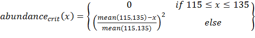
(1) 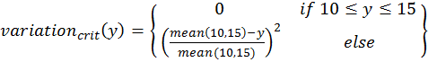
(2) 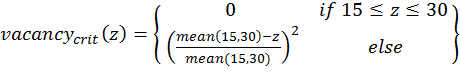
(3) 
(4) with x,y,z being the corresponding simulation result, e.g., x is the mean abundance of the simulation as mentioned above. If the simulation result is within the acceptable range, the cost value of the criteria becomes 0; otherwise, it is the squared relative deviation. By squaring the deviations, we keep the values positive and weigh large deviations disproportionately higher than low deviations (Eqs. 1–3). This has an important effect on Eq. 4. For example, if we find small deviations in all three criteria, the overall cost value (Eq. 4) still stays low, but when only one criterion's deviation is rather high, its criterion value and therefore also the overall cost value becomes disproportionately high. We use this approach here because we think that small deviations in all criteria are less important than a single large deviation.
- 2.12
- Alternatives to this are multi-criterion approaches where each criterion is considered separately and a combined assessment is performed by determining Pareto optima or fronts (Miettinen 1999; Weck 2004). See, for example, the package mco (Trautmann et al. 2013) for Pareto optimisation with a genetic algorithm. Multi-criterion approaches, however, have their own challenges and limitations and are much less straightforward to use than the cost function approach that we used here.
- 2.13
- Because the example model includes stochastic effects, we repeat model runs using the same initialisation and average the output. Following Martínez et al. (2011) and Kerr et al. (Kerr 2002), we ran 10 repetitions for every tested parameter set. However, for "real" simulation studies it is advisable to determine the number of repetitions by running the model with an increasing number of repetitions and calculating the resulting coefficient of variation (CV) of the simulation output. At the number of repetitions where the CV remains (nearly) the same, convergence can often be assumed (Lorscheid et al. 2012). However, in cases of non-linear relationships between the input parameters and simulation output, this assumption may not be fulfilled.
- 2.14
- If we have replicates of observational data and a stochastic model, which is not the case for our example, we should compare distributions of the results rather than using a single value comparison, as recommended in Stonedahl & Wilensky (2010). The calculation of the pomdev measure (Piou et al. 2009), which is already implemented in the R package Pomic (Piou et al. 2009), could be of interest in such a case.
- 2.15
- If we want to compare whole time series instead of single output values, the aggregation procedure can become more difficult. Such data could also be compared by mean square deviations (see, for example, Wiegand et al. 1998), but then small differences in all measurement points can yield the same deviation as a strong difference in one point. Hyndman (2013) provides an overview of R packages helpful for time series analysis.
Full factorial design
- 2.16
- A systematic method for exploring parameter space is (full) factorial design, known from Design of Experiments (DoE) methodology (Box et al. 1978). It can be applied if the model runs very quickly or if the numbers of unknown parameters and possible parameter values are rather small. For example, Jakoby et al. (2014) ran a deterministic generic rangeland model that includes nine parameters and a few difference equations for one billion parameter sets.
- 2.17
- In DoE terminology, the independent variables are termed "factors" and the dependent (output) variables "responses". For full factorial design, all possible factor combinations are used. The critical point here is to define the possible factor levels (parameter values) within the parameter ranges. For parameter values that are integer values by nature (e.g., number of children) this is easy, but for continuous values it can be difficult to find a reasonable step size for the factor levels. This can be especially difficult if the relationship between the factor and the response variables is non-linear.
- 2.18
- For our example model, we assume the following factor levels (taken from Railsback & Grimm 2012):
- scout-prob: 0.0 to 0.5 with step size 0.05
- survival-prob: 0.95 to 1.0 with step size 0.005
# 1. Define a function that runs the simulation model
We include this example because it is a good starting point for proceeding to more sophisticated methods, such as the fractional factorial design. If you want to use a classical full factorial design with NetLogo, we recommend using NetLogo's "BehaviorSpace" (Wilensky & Shargel 2002).
# for a given parameter combination and returns the
# value(s) of the fitting criteria. See Supplementary
# Material (simulation_function1.R) for an
# implementation example using RNetLogo.
sim <- function(params) {
...
return(criteria)
}
# 2. Create the design matrix.
full.factorial.design <- expand.grid(scout.prob =
seq(0.0,0.5,0.05), survival.prob = seq(0.95,1.0,0.005))
# 3. Iterate through the design matrix from step 2 and call
# function sim from step 1 with each parameter combination.
sim.results <- apply(full.factorial.design, 1, sim)
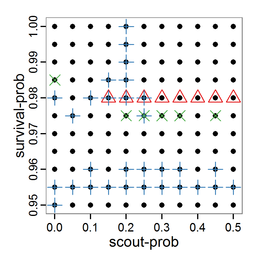
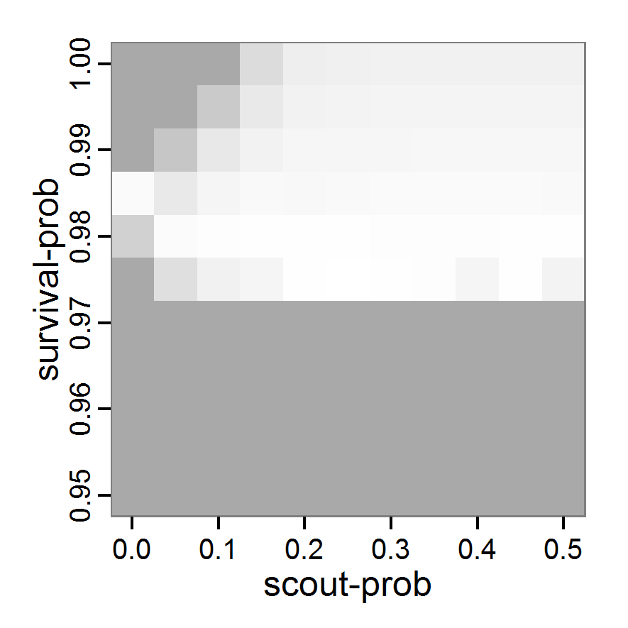
Figure 1. Left: Results of the full factorial design (121 parameter sets) using categorical evaluation criteria. Black points symbolise the tested parameter combinations, and the three different symbols show whether the evaluation criteria were met (red triangle: abundance criterion, blue cross: variation criterion, green x: vacancy criterion). Right: Results of the full factorial design based on conditional best-fit equations (Equation 1 to 3), summed up to the one metric cost (Equation 4). The cost values are truncated at 10.0 (max. cost value was 842). Grey cells indicate high cost values, and white cells represent low values, i.e., better solutions. One cell represents one simulation with parameter values from the cell's midpoint corresponding to the left panel. The results of the model calibration procedure with categorical calibration criteria can be explored visually. Figure 1 (left panel) shows such a figure for the example model. We see that none of the 121 tested parameter combinations met the three calibration criteria simultaneously. Still, the figure provides some useful hints. The central region of parameter space appears to be promising. The failure to meet all three criteria simultaneously might be due to the step width used.
- 2.19
- Using the same output data that underlie Figure 1 (left panel), we can calculate the conditional best-fit equations (Eq. 4) and plot the results as a raster map (Figure 1, right panel). This plot shows more directly than the left panel where the most promising regions of parameter space are located (the white cells), which can then be investigated in more detail.
- 2.20
- Overall, full factorial design is useful for visually exploring model behaviour regarding its input parameters in a systematic way but only if the number of parameters and/or factor levels is low. To gain a coarse overview, full factorial design can be useful for calibrating a small number of parameters at a time because the number of combinations can be kept small enough. Fractional factorial designs can be used for a larger number of parameters by selecting only a subset of the parameter combinations of a full factorial design (Box et al. 1978); the application in R is very similar, see the above-mentioned collection by Groemping (2013a).
Classical sampling methods
- 2.21
- One common method of avoiding full factorial designs, both in simulations and in real experiments, is the usage of sampling methods. The purpose of these methods is to strongly reduce the number of parameter sets that are considered but still scan parameter space in a systematic way. Various algorithms exist to select values for each single parameter, for example, random sampling with or without replacement, balanced random design, systematic sampling with random beginning, stratified sampling etc.
Simple random sampling
- 2.22
- The conceptually and technically simplest, but not very efficient, sampling method is simple random sampling with replacement. For each sample of the chosen sample size (i.e., number of parameter sets), a random value (from an a priori selected probability density function) is taken for each parameter from its value range. The challenge here, and also for all other (random) sampling methods, is finding an appropriate probability density function (often just a uniform distribution is used) and the selection of a useful sample size. Applying a simple random sampling in R can look like the following:
# 1. Define a simulation function (sim) as done for
# Full factorial design.
# 2. Create the random samples from the desired random
# distribution (here: uniform distribution).
random.design <- list('scout-prob'=runif(50,0.0,0.5),
'survival-prob'=runif(50,0.95,1.0))
# 3. Iterate through the design matrix from step 2 and call
# function sim from step 1 with each parameter combination.
sim.results <- apply(as.data.frame(random.design), 1, sim) - 2.23
- Despite the fact that this simple random sampling is not an efficient method and could rather be considered a trial-and-error approach to exploring parameter space, it is used quite often in practice (e.g., Molina et al. 2001). We nevertheless included the source code for this example in the Supplementary Material because it can be easily adapted to other, related sampling methods.
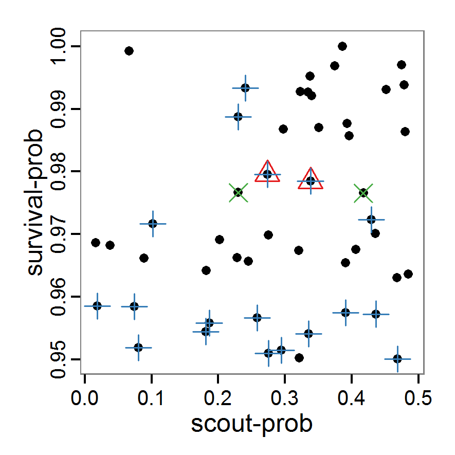
Figure 2. : Results of using simple random sampling based on categorical calibration criteria with 50 samples. Black points symbolise the tested parameter combinations, and the three different symbols show whether the evaluation criteria were met (red triangle: abundance criterion, blue cross: variation criterion, green x: vacancy criterion). - 2.24
- The results of an example application using 50 samples with categorical calibration criteria are shown in Figure 2. The sampling points are distributed over the parameter space but leave large gaps. The overall pattern of the regions where the different criteria were met looks similar to that of the full factorial design (Figure 1). In this example application, we were not able to find a parameter combination that meets all three evaluation criteria. In general, the simple random sampling method is not an efficient method for parameter fitting.
Latin hypercube sampling
- 2.25
- As a more efficient sampling technique to scan parameter spaces, Latin hypercube sampling (LHS) (McKay et al. 1979) is widely used for model calibration and sensitivity analysis as well as for uncertainty analysis (e.g., Marino et al. 2008; Blower & Dowlatabadi 1994; Frost et al. 2009; Meyer et al. 2009). LHS is a stratified sampling method without replacement and belongs to the Monte Carlo class of sampling methods. It requires fewer samples to achieve the same accuracy as simple random sampling. The value range of each parameter is divided into N intervals (= sample size) so that all intervals have the same probability. The size of each interval depends on the used probability density distribution of the parameter. For uniform distributions, they all have the same size. Then, each interval of a parameter is sampled once (Marino et al. 2008). As there are some packages for creating Latin hypercubes available in R, such as tgp (Gramacy & Taddy 2013) and lhs (Carnell 2012), it is easy to use this sampling method. For our small example model, the code for generating a Latin hypercube with the tgp package is as follows:
# 1. Define a simulation function (sim) as done for
# Full factorial design.
# 2. Create parameter samples from a uniform distribution
# using the function lhs from package tgp.
param.sets <- lhs(n=50, rect=matrix(c(0.0,0.95,0.5,1.0), 2))
# 3. Iterate through the parameter combinations from step 2
# and call function sim from step 1 for each parameter
# combination.
sim.results <- apply(as.data.frame(param.sets), 1, sim) - 2.26
- As with simple random sampling, the challenge of choosing appropriate probability density distributions and a meaningful sample size remains. Using, as shown above, a uniform random distribution for the two parameters of our example model, the results using categorical criteria for 50 samples are shown in Figure 3. We have been lucky and found one parameter combination (scout-prob: 0.0955, survival-prob: 0.9774) that met all three criteria. The source code for creating a Latin hypercube in the Supplementary Material also includes an example of applying a best-fit calibration (Eq. 4).
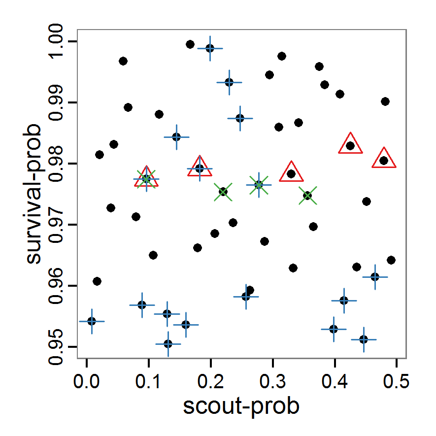
Figure 3. Results from the Latin hypercube sampling using categorical evaluation criteria with 50 samples. Black points symbolise tested parameter combinations, and the three different symbols show whether the evaluation criteria were met (red triangle: abundance criterion, blue cross: variation criterion, green x: vacancy criterion). Optimisation methods
- 2.27
- In contrast to the sampling methods described above, optimisation methods create parameter sets not before the simulations are started but in a stepwise way based on the results obtained with one or more previously used parameter sets. These methods are used in many different disciplines, including operations research, physics etc. (Aarts & Korst 1989; Bansal 2005). As the relationships between the input parameters and the output variables in ABMs are usually non-linear, non-linear heuristic optimisation methods are the right choice for parameter fitting. We will give examples for gradient and quasi-Newton methods, simulated annealing and genetic algorithms. There are, however, many other optimisation methods available, such as threshold accepting, ant colony optimisation, stochastic tunnelling, tabu search etc.; several packages for solving optimisation problems are available in R. See Theussl (2013) for an overview.
Gradient and quasi-Newton methods
- 2.28
- Gradient and quasi-Newton methods search for a local optimum where the gradient of change in parameters versus change in the fitting criterion is zero. In cases where multiple local optima exist, the ability to find the global optimum depends on the starting conditions (Sun & Yuan 2006). A popular example of gradient methods is the so-called conjugate gradient method (CG). Because the standard CG is designed for unconstrained problems (i.e., the parameter space cannot be restricted to a specific value range), it is not useful to apply it to parameter estimation problems of ABMs. Quasi-Newton methods instead are based on the Newton method but approximate the so-called Hessian matrix and, therefore, do not require the definition of the second derivative (Biethahn et al. 2004). An introduction to these methods can be found in Fletcher (1987). The implementation of both the gradient and quasi-Newton methods requires a gradient function to be supplied, which is often difficult in ABMs. Implementations in R can often approximate the gradient numerically. Here, we selected the L-BFGS-B method by Byrd et al. (1995), which is a variant of the popular Broyden–Fletcher–Goldfarb–Shanno (BFGS) method (Bonnans et al. 2006) because it is the only method included in the function optim of R's stats package (R Core Team 2013a), which can take value ranges (upper and lower limits) for the parameters into account. The strength of the L-BFGS-B method is the ability to handle a large number of variables. To use the L-BFGS-B method with our example ABM, we must define a function that returns a single fitting criterion for a submitted parameter set. For this, we use the single fitting criterion defined in Eq. 4. The usage of this method is as follows:
# 1. Define a function that runs the simulation model
# for a given parameter combination and returns the
# value of the (aggregated) fitting criterion. See
# Supplementary Material (simulation_function2.R) for
# an implementation example using RNetLogo.
sim <- function(params) {
...
return(criterion)
}
# 2. Run L-BFGS-B. Start, for example, with the maximum of
# the possible parameter value range.
result <- optim(par=c(0.5, 1.0),
fn=sim, method="L-BFGS-B",
control=list(maxit=200),
lower=c(0.0, 0.95), upper=c(0.5, 1.0)) - 2.29
- Other packages useful for working with gradient or quasi-Newton methods are Rcgmin (Nash 2013), optimx (Nash & Varadhan 2011) and BB (Varadhan & Gilbert 2009). The source code, including the L-BFGS-B, is in the Supplementary Material and can easily be adapted for other gradient or quasi-Newton methods.
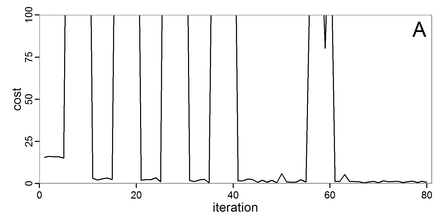
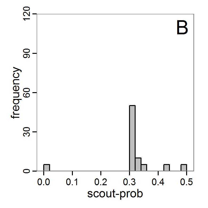
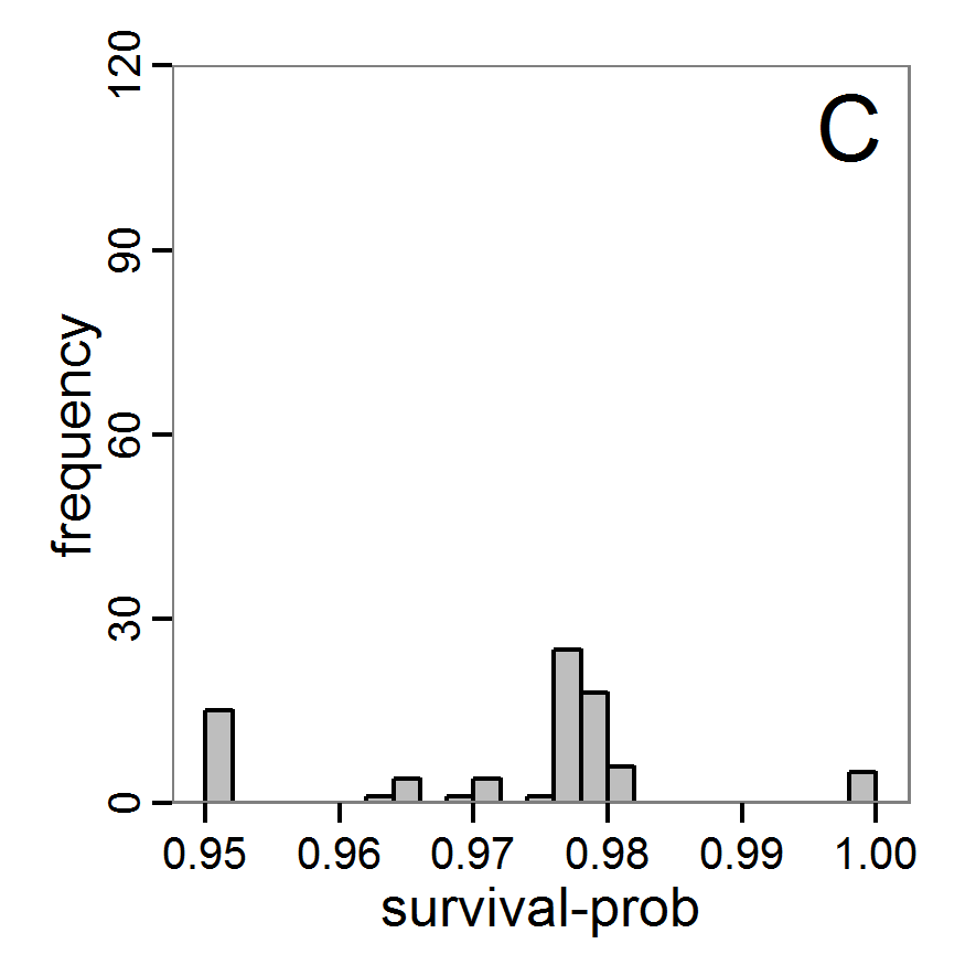
Figure 4. Results of the L-BFGS-B method (includes intermediate simulations, e.g., simulations for gradient approximation). A: Performance of the cost value (Eq. 4) over the calls of the simulation function (x-axis, truncated at cost value 100, max. cost value was 317). B: Histogram of the tested parameter values for parameter scout-prob. C: Histogram of the tested parameter values for parameter survival-prob. - 2.30
- The variation of the aggregated value of the conditional equations (cost value) over the 80 model evaluations (including evaluations for gradient approximation) of the L-BFGS-B method is shown in Figure 4 (upper panel). The algorithm checks the cost value of the start parameter set and the parameter values at the bounds of the valid parameter values, resulting in strong variations of the cost value over the number of iterations. Another source of the strong variation is intermediate simulation for the approximation of the gradient function. As we are only interested in the regions with low cost values, we truncated the high cost values in the graph to obtain a more detailed look at the variation of the lower cost values over the iterations. The lower panels of Figure 4 show the histograms of the tested parameter values. We see that the search by the L-BFGS-B method for an optimal value for both model parameters, in the configuration used here, shortly checked the extreme values of the value range but focused on the middle range of the parameter space. We see that the method stopped quickly and left large areas out of consideration, which is typical for methods searching for local optima without the ability to also accept solutions with higher costs during the optimisation. For survival-prob, the minimum possible value is checked more precisely and smaller parts of the parameter space remain untested. The best fit was found with parameter values of 0.3111 for scout-prob and 0.9778 for survival-prob, which resulted in a cost value of 1.1. This cost value indicates that the three categorical criteria were not matched simultaneously; otherwise the cost value would be zero. However, keep in mind that the application of the method was not fine-tuned and a finite-difference approximation was used for calculating the gradient.
Simulated annealing
- 2.31
- In simulated annealing, temperature corresponds to a certain probability that a local optimum can be left. This avoids the problem of optimisation methods becoming stuck in local, but not global, optima. Simulated annealing is thus a stochastic method designed for finding the global optimum (Michalewicz & Fogel 2004).
- 2.32
- There are several R packages that include simulated annealing functions, for example, stats (R Core Team 2013a), subselect (Cerdeira et al. 2012) or ConsPlan (VanDerWal & Januchowski 2010). As for the gradient and quasi-Newton methods, to use simulated annealing with an ABM we must define a function that returns a single fitting criterion for a submitted parameter set. Using the GenSA package (Xiang et al. forthcoming), which allows one to define value ranges for the parameters, running a simulated annealing optimisation looks like this:
# 1. Define a simulation function (sim) as done for the
# L-BFGS-B method.
# 2. Run SA algorithm. Start, for example, with the maximum
# of the possible parameter value range.
result <- GenSA(par=c(0.5,1.0), fn=sim,
lower=c(0.0, 0.95), upper=c(0.5, 1.0)) - 2.33
- As with the gradient and quasi-Newton methods, the choice of the starting values as well as the number of iterations can be challenging. Furthermore, specific to simulated annealing, the selection of an appropriate starting temperature is another critical point.
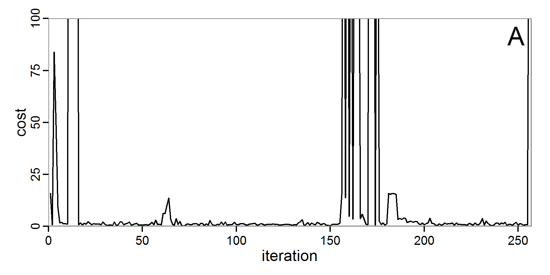
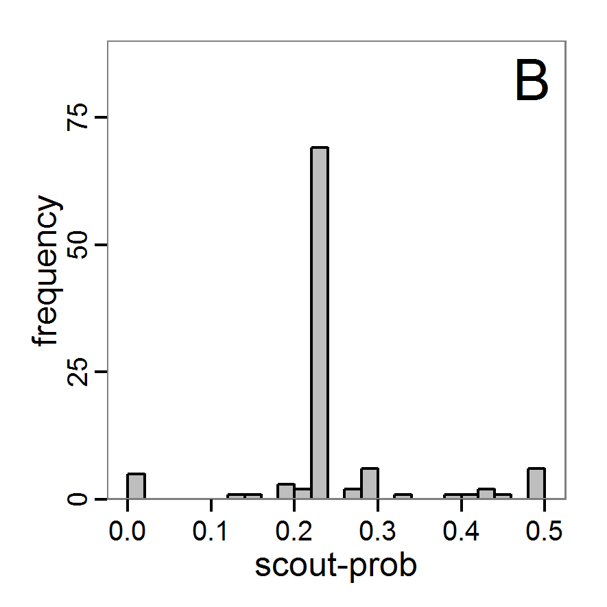
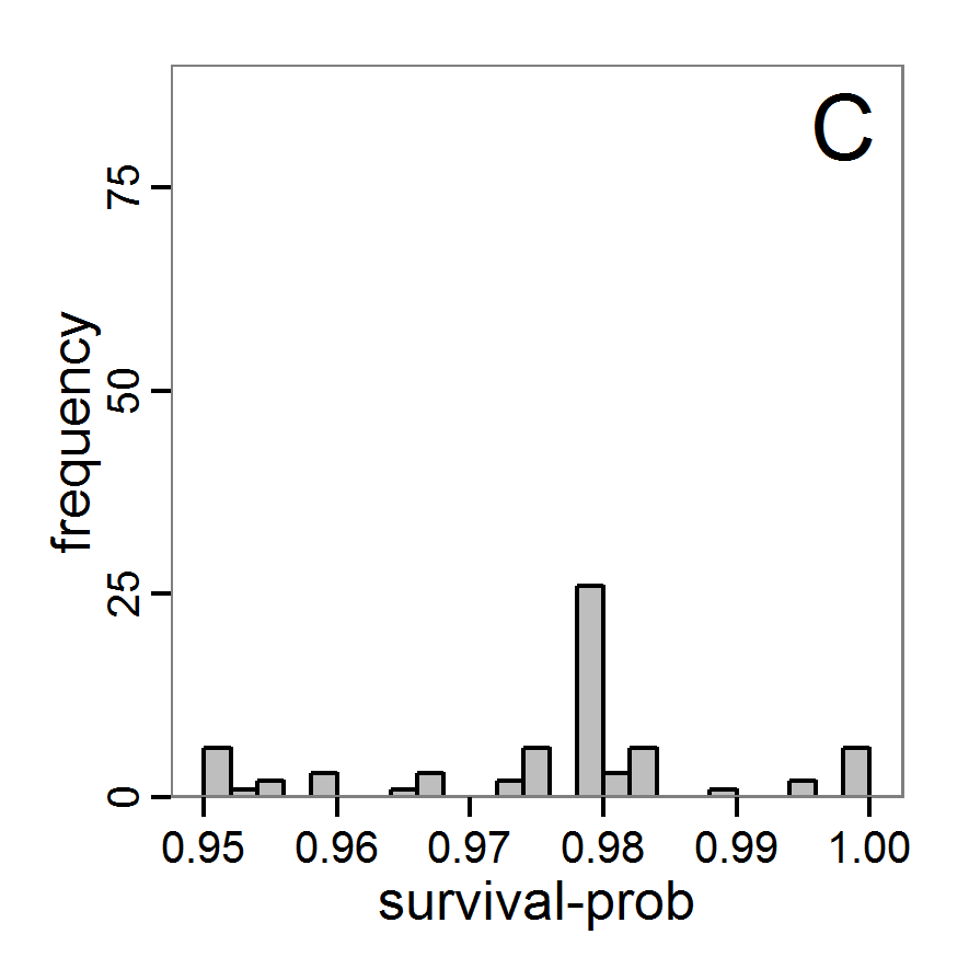
Figure 5. Results of the simulated annealing method. A: Performance of the cost value (Eq. 4) over the calls of the simulation function (x-axis, truncated at cost value 100, max. cost value was 317). B: Histogram of the tested parameter values for parameter scout-prob. C: Histogram of the tested parameter values for parameter survival-prob. - 2.34
- The result of an application example with 256 model evaluations is shown in Figure 5. In the upper panel, we see the variation of the cost value over the iterations, i.e., the simulation function calls. The algorithm found a good solution very fast, but then the algorithm leaves this good solution and also accepts less good intermediate solutions. Because we are primarily interested in the regions with low cost values, i.e., good adaptations of the model to the data, we truncated the graph to obtain a better view of the variation in the region of low cost values. In the lower panels, we see that more of the parameter space is tested than with the previous L-BFGS-B method (Figure 4). The focus is also in the middle range of the parameter space, which is the region where the best solution was found and which is the most promising part of the parameter space, as we already know from the full factorial design. The minimum cost value found in this example was 0.65 with corresponding parameter values of 0.225 for scout-prob and 0.9778 for survival-prob. As with the quasi-Newton method, the cost value indicates that the three criteria have not been met simultaneously.
Evolutionary or genetic algorithms
- 2.35
- Evolutionary algorithms (EA) are inspired by the natural process of evolution and feature inheritance, selection, mutation and crossover. Genetic algorithms (GA) are, like evolutionary strategies, genetic programming and some other variants, a subset of EAs (Pan & Kang 1997). GAs are often used for optimisation problems by using genetic processes such as selection or mutation on the parameter set. The parameter set, i.e., a vector of parameter values (genes), corresponds to the genotype. A population is formed by a collection of parameter sets (genotypes). Many books and articles about this methodology are available, e.g., Mitchell (1998), Holland (2001), or Back (1996). Application examples of EA/GA for parameter estimation in the context of ABMs can be found in Duboz et al. (Duboz 2010), Guichard et al. (2010), Calvez & Hutzler (2006), or Stonedahl & Wilensky (2010).
- 2.36
- There are several packages for evolutionary and genetic algorithms available in R; see the listing in Hothorn (2013). Using the package genalg (Willighagen 2005) enables us to take ranges of permissible values for the parameters into account. The rbga function of this package requires a function that returns a single fitting criterion, as we have also used for the quasi-Newton and simulated annealing methods. The procedure in R is as follows:
# 1. Define a simulation function (sim) as done for the
# L-BFGS-B method.
# 2. Run the genetic algorithm.
result <- rbga(stringMin=c(0.0, 0.95),
stringMax=c(0.5, 1.0),
evalFunc=sim, iters=200)
- 2.37
- Challenges with EAs/GAs include selecting an appropriate population size and number of iterations/generations, as well as meaningful probabilities for various genetic processes, such as mutation.
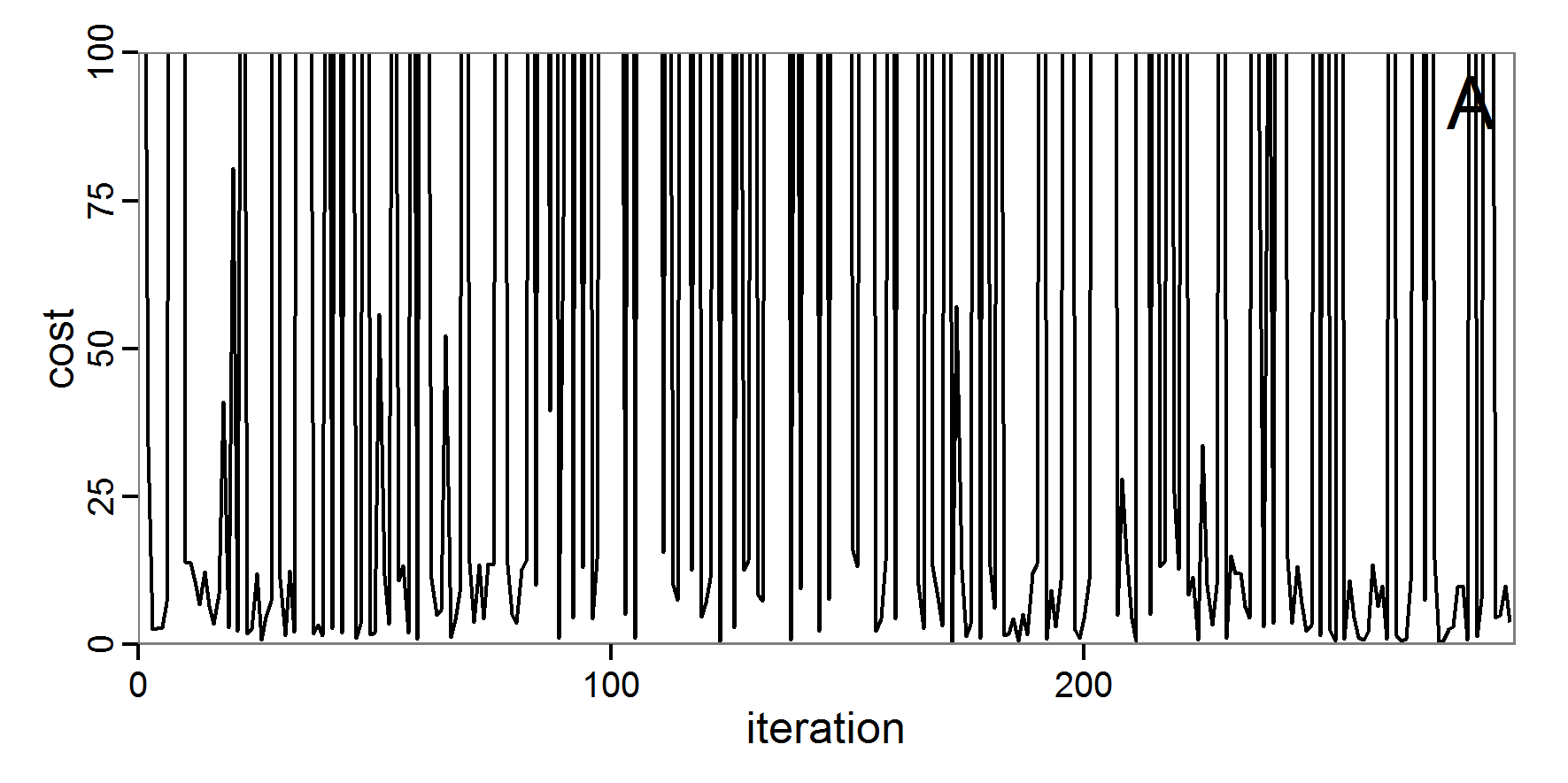
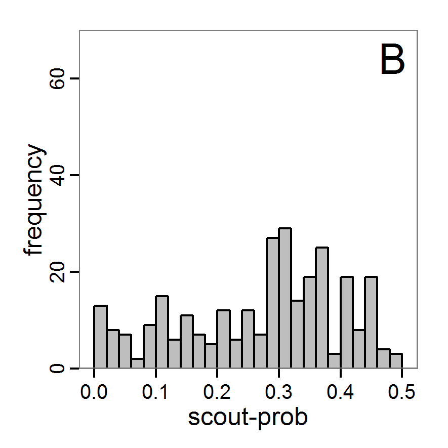
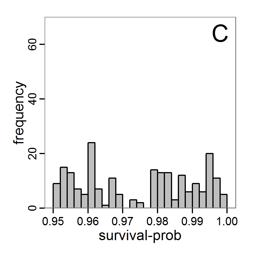
Figure 6. Results of the genetic algorithm method for 10 populations and 50 generations. A: Performance of the cost value (Eq. 4) over the calls of the simulation function (x-axis, truncated at cost value 100, max. cost value was 2923). B: Histogram of the tested parameter values for parameter scout-prob. C: Histogram of the tested parameter values for parameter survival-prob. - 2.38
- The fitting process using the genalg package with 290 function evaluations resulted in a best cost value of 0.35 with scout-prob of 0.3410 and survival-prob of 0.9763. The performance of the cost value over the model evaluations is shown in the upper panel of Figure 6. We find a very strong oscillation because successive runs are more independent than in the other methods above, e.g., by creating a new population. Therefore, this graph looks much more chaotic, and truncating the vertical axis to zoom into the region of low cost values is less informative in this specific case. As we can see in the lower panels of the figure, a wide range of parameter values has been tested, with slightly higher frequency around the best parameter value for scout-prob and a more diffuse pattern for survival-prob. However, the best parameter combination found is very similar to the one found by the other optimisation methods. In general, it appears that the promising value range of survival-prob is much smaller than that for scout-prob. The values of (sub-) optimal solutions for survival-prob are always close to 0.977, whereas the corresponding value of scout-prob varies on a much wider value range with only a small influence on the cost value. This pattern was already shown in Figure 1 (right panel). For investigating such a pattern in more detail, Bayesian methods can be very help- and powerful, as presented below.
Bayesian methods
- 2.39
- Classical statistical maximum likelihood estimation for model parameters cannot be applied to complex stochastic simulation models; the likelihood functions are either intractable or hard to detect because this is computationally too expensive (Jabot et al. 2013). By using the Bayesian strategy, the true/posterior probability density functions of parameters are calculated by point-wise likelihood approximations across the parameter space. The basic idea, as described in Jabot et al. (2013), is to run the model a very large number of times with different parameter values drawn from distributions we guess are underlying (prior distributions). Then, the simulation results and the observational data are compared using so-called summary statistics, which are some aggregated information calculated from the simulation and the observational data to reduce the dimensionality of the data. Only those parameter values where the difference between the simulated and the observed summary statistics is less than a defined threshold (given by a tolerance rate) are kept. At the end, an approximation of the posterior distribution is formed by the retained parameter values. Such methods, called Approximate Bayesian Computing (ABC), have been increasingly used for simulation models in recent years (e.g., May et al. 2013; Martínez et al. 2011; Sottoriva & Tavaré 2010; and review by Hartig et al. 2011). They not only deliver a best estimate for the parameter values but also provide measures of uncertainty with consideration of correlations among the parameters (Martínez et al. 2011). Introductions to Bayesian statistical inference using ABC can be found in Beaumont (2010), Van Oijen (2008), or Hartig et al. (2011).
- 2.40
- A list of useful R packages around Bayesian inference can be found in Park (2012). The most relevant packages regarding ABC are abc (Csillery et al. 2012), EasyABC (Jabot et al. 2013), pomp (King et al. 2013), FME (Soetaert & Petzoldt 2010) and MCMChybridGP (Fielding 2011). If a specific method is not available in an out-of-box package, there are several R packages that can assist in developing custom implementations, such as the MCMC package (Geyer & Johnson 2013) with its Markov chain Monte Carlo Metropolis-Hastings algorithm or the coda package (Plummer et al. 2006) for the analysis of Markov chain Monte Carlo results. An R interface to the openBUGS software (Lunn et al. 2009) comes with the BRugs package (Thomas et al. 2006) and enables the advanced user to define models and run Bayesian approximations in openBUGS, which is beyond the scope of this paper. MCMC in an ABC framework can also be used to compute some measures of model complexity (Piou et al. 2009). The Pomic package (Piou et al. 2009) is based on an adaptation of the DIC measure (Spiegelhalter et al. 2002) to compare the goodness of fit and complexity of ABMs developed in a POM context.
- 2.41
- Note that Bayesian methods require deeper knowledge and understanding than the other methods presented above to be adapted properly to a specific model. The methods presented above could be understood in principle without previous knowledge, but this is not the case for Bayesian methods. We recommend first reading Wikipedia or other introductions to these methods before trying to use the methods described in this section. Nevertheless, even for beginners, the following provides an overview of the inputs, packages, and typical outputs of Bayesian calibration techniques.
Rejection and regression sampling
- 2.42
- The easiest variant of ABC regarding the sampling scheme is rejection sampling. Here, the user first defines a set of summary statistics, which are used to compare observations with simulations. Furthermore, a tolerance value, which is the proportion of simulation points whose parameter set is accepted, must be selected. Then, parameter sets are drawn from a user-defined prior distribution and tested for acceptance. At the end, the posterior distribution is approximated from the accepted runs (Beaumont et al. 2002).
- 2.43
- Such sampling can be performed in R using the package abc (Csillery, Blum et al. 2012) or the package EasyABC (Jabot et al. 2013). The abc package offers two further improvements to the simple rejection method based on Euclidean distances: a local linear regression method and a non-linear regression method based on neural networks. Both add a further step to the approximation of the posterior distribution to correct for imperfect matches between the accepted and observed summary statistics (Csillery, Francois et al. 2012).
- 2.44
- Because the abc package expects random draws from the prior distributions of the parameter space, we must create such an input in a pre-process. For this, we can, for simplicity, reuse the code of the Latin hypercube sampling with separate best-fit measures for all three fitting criteria used as summary statistics (see Eqs. 1–3). Also for simplicity, we apply a non-informative uniform (flat) prior distribution (for further reading see Hartig et al. 2011). As summary statistics, we use the three criteria defined in the model description. We assume that the observed summary statistics is calculated as the mean of the minimum and the maximum of the accepted output value range, i.e., we assume that the value range was gained by two field measurements and we use the mean of these two samples to compare it with the mean of two simulated outputs. The procedure of using the abc function in R (for simple rejection sampling) is as follows:
# 1. Run a Latin hypercube sampling as performed above.
# The result should be two variables, the first
# containing the parameter sets (param.sets) and
# the second containing the corresponding summary
# statistics (sim.sum.stats).
# 2. Calculate summary statistics from observational data
#(here: using the mean of value ranges).
obs.sum.stats <- c(abundance=mean(c(115,135)),
variation=mean(c(10,15)),
vacancy=mean(c(0.15,0.3)))
# 3. Run ABC using observations summary statistics and the
# input and output of simulations from LHS in step 1.
results.abc <- abc(target=obs.sum.stats, param=param.sets,
sumstat=sim.sum.stats,
tol=0.3, method="rejection")
- 2.45
- The results, i.e., the accepted runs that form the posterior distribution of simple rejection sampling and of the local linear regression method, can be displayed using histograms, as presented in Figure 7 (upper and middle panels). These results are based on Latin hypercube sampling with 30,000 samples and a tolerance rate of 30 per cent, which defines the percentage of accepted simulations. The histograms can be used to estimate the form of the probability density function (kernel density), which is shown in the lower panels of Figure 7. These density estimations can be taken subsequently to gain distribution characteristics for the two input parameters, as shown in Table 2. Afterwards, the density estimations can be used to run the model not only with the mean or median of the parameter estimation but also for an upper and lower confidence value, which would result not only in one model output but in confidence bands for the model output. See Martínez et al. (2011) for an example.
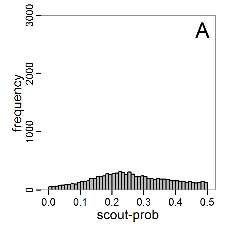
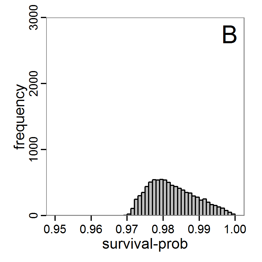
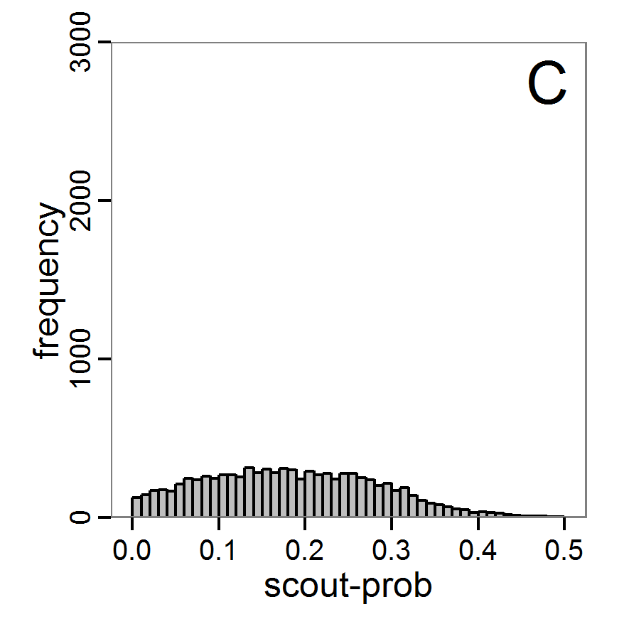
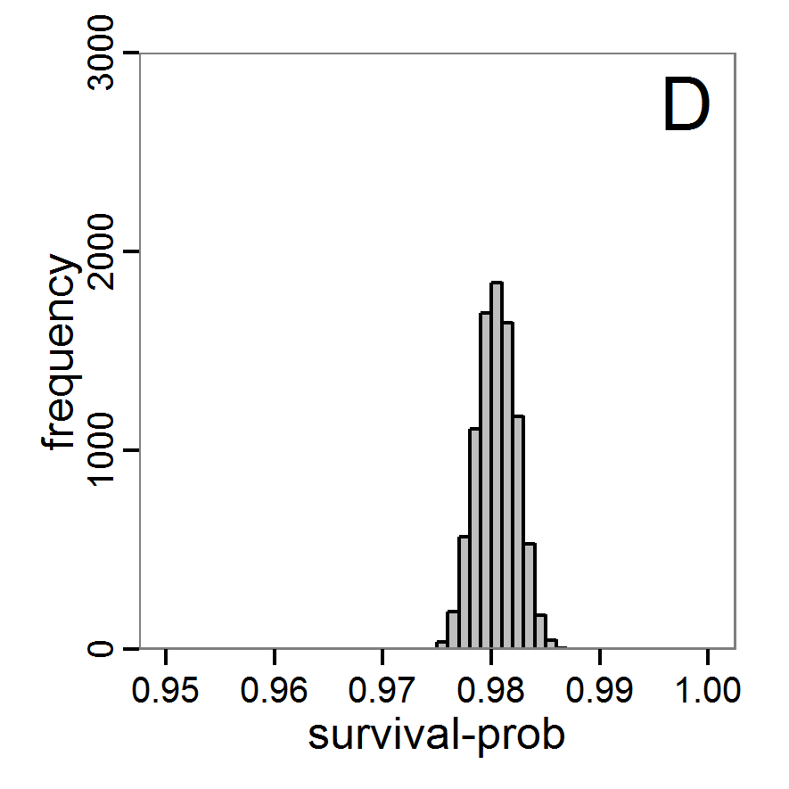
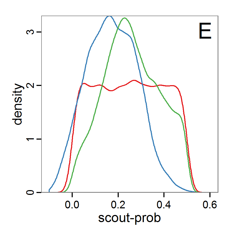
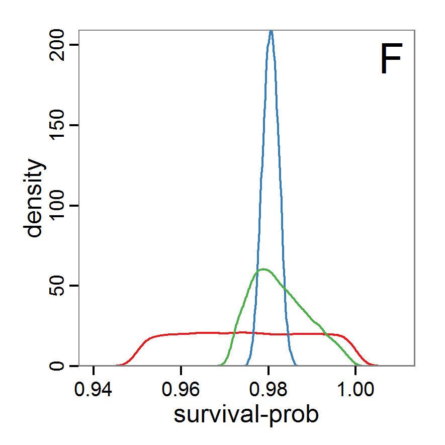
Figure 7. Posterior distribution generated with the ABC rejection sampling method as well as the rejection sampling method followed by additional local linear regression. A: Histogram of accepted runs for scout-prob using rejection sampling. B: Histogram of accepted runs for survival-prob using rejection sampling. C: Histogram of accepted runs for scout-prob using the local linear regression method. D: Histogram of accepted runs for survival-prob using the local linear regression method. E & F: Density estimation for scout-prob (E) and survival-prob (F) by rejection sampling (green line), by the local linear regression method (blue line) and from a prior distribution (red line). - 2.46
- We see that there are considerable differences in results between the simple rejection sampling and the rejection sampling with local linear regression correction. For example, the mean value of scout-prob is much lower with the regression method than with the simple rejection method. Furthermore, the posterior distribution of survival-prob is narrower with the regression method than with the simple rejection method.
Table 2: Posterior distribution characteristics for the two parameters gained from the ABC rejection sampling (first and third columns) and the local linear regression method (second and fourth columns; weighted). scout-prob survival-prob rej. sampl. loc. lin. reg. rej. sampl. loc. lin. reg. Minimum 0.0003 -0.1151 0.9695 0.9746 5% percentile 0.0622 -0.0185 0.9733 0.9774 Median 0.2519 0.1423 0.9817 0.9803 Mean 0.2596 0.1485 0.9826 0.9803 Mode 0.2270 0.0793 0.9788 0.9805 95% percentile 0.4666 0.3296 0.9946 0.9832 Maximum 0.5000 0.5261 0.9999 0.9863 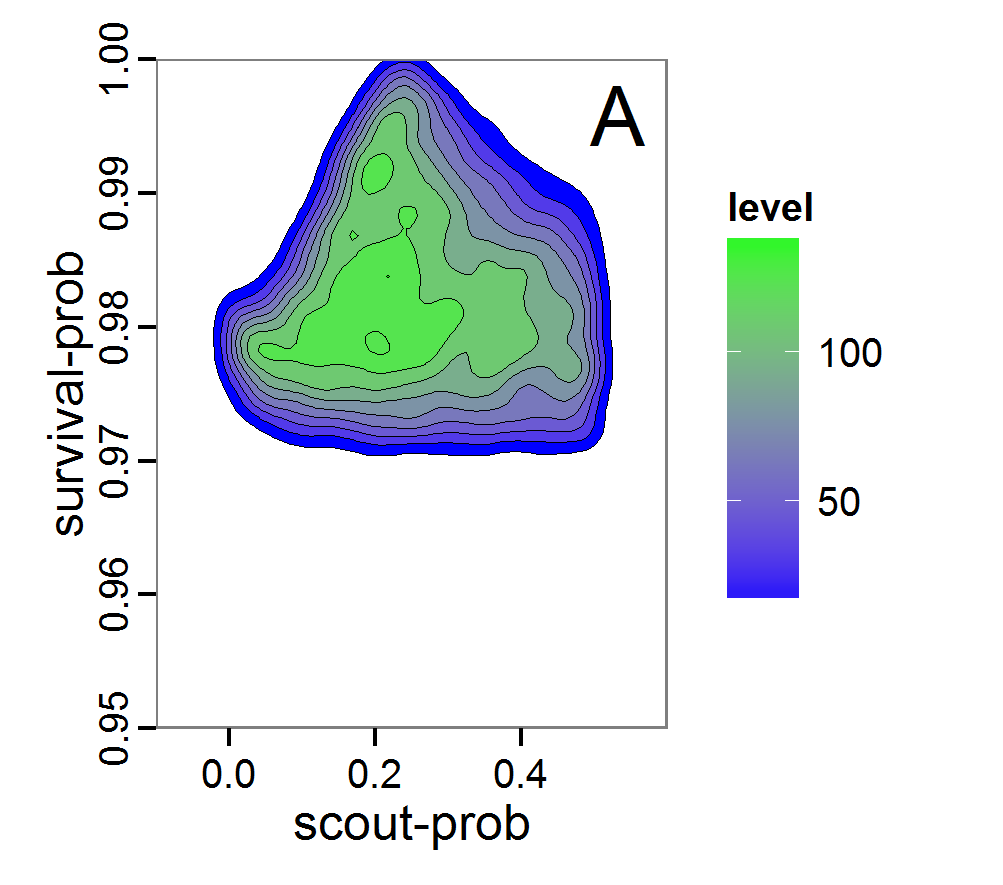
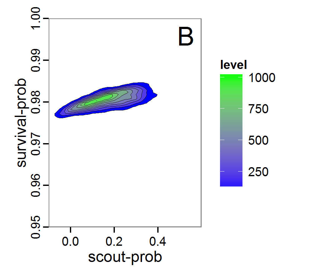
Figure 8. Joint posterior density estimation based on A: ABC rejection sampling, B: rejection sampling with additional local linear regression. Both with 10–90% highest density contours. The last contour is invisible without zooming in, meaning high density is concentrated in a small area. - 2.47
- Looking at the joint posterior density in Figure 8, we see how the densities of the two parameters are related to each other. Not surprisingly, we see strong differences for the two methods, as we already know from Figure 7 that the distributions differ. However, we also see that the additional local linear regression condenses the distribution very much and uncovers a linear correlation between the two parameters. A Spearman correlation test between the two parameter samples delivers a ρ of 0.66 (p-value < 2.2e-16) for the method with the additional local linear regression, whereas ρ is only 0.02 (p-value =0.11) for the simple rejection sampling. This result for the method with the additional local linear regression is in good accordance with the results of the following method and has many similarities to the pattern we know from the results of the full factorial design (Figure 1, right panel).
- 2.48
- Because the application of the additional local linear regression method is based on the same simulation results as the simple rejection sampling, it comes with no additional computational costs. Therefore, it is a good idea to run both methods and check their convergence.
Markov chain Monte Carlo
- 2.49
- Markov chain Monte Carlo (MCMC) is an efficient sampling method where the selection of the next parameter combination depends on the last parameter set and the resulting deviation between the simulation and the observation (Hartig et al. 2011). Therefore, sampling is concentrated in the regions with high likelihood. This makes the method more efficient in comparison with rejection sampling. Only the initial parameter set is drawn from the prior distribution. In the long run, the chain of parameter sets will converge to the posterior distribution. The advantage of the MCMC methods over the rejection sampling methods is that it does not sample from the prior distribution. See, for example, Beaumont (2010) for further reading.
- 2.50
- The R package EasyABC (Jabot et al. 2013) delivers several different algorithms for performing coupled ABC-MCMC schemes. The usage in R looks like this:
# 1. Define a function that runs the simulation model for a
# given parameter combination and returns all summary
# statistics.
# See Supplementary Material (simulation_function4.R)
# for an implementation example using RNetLogo.
sim <- function(params) {
...
return(sim.sum.stats)
}
# 2. Calculate summary statistics from observational data
# (here using the mean of ranges).
obs.sum.stats <- c(abundance=mean(c(115,135)),
variation=mean(c(10,15)),
vacancy=mean(c(0.15,0.3)))
# 3. Generate prior information.
prior <- list('scout-prob'=c("unif",0.0,0.5),
'survival-prob'=c("unif",0.95,1.0))
# 4. Run ABC-MCMC.
results.MCMC <- ABC_mcmc(method="Marjoram", model=sim,
prior=prior, summary_stat_target=obs.sum.stats)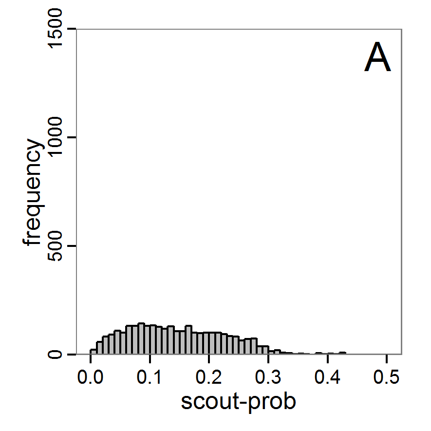
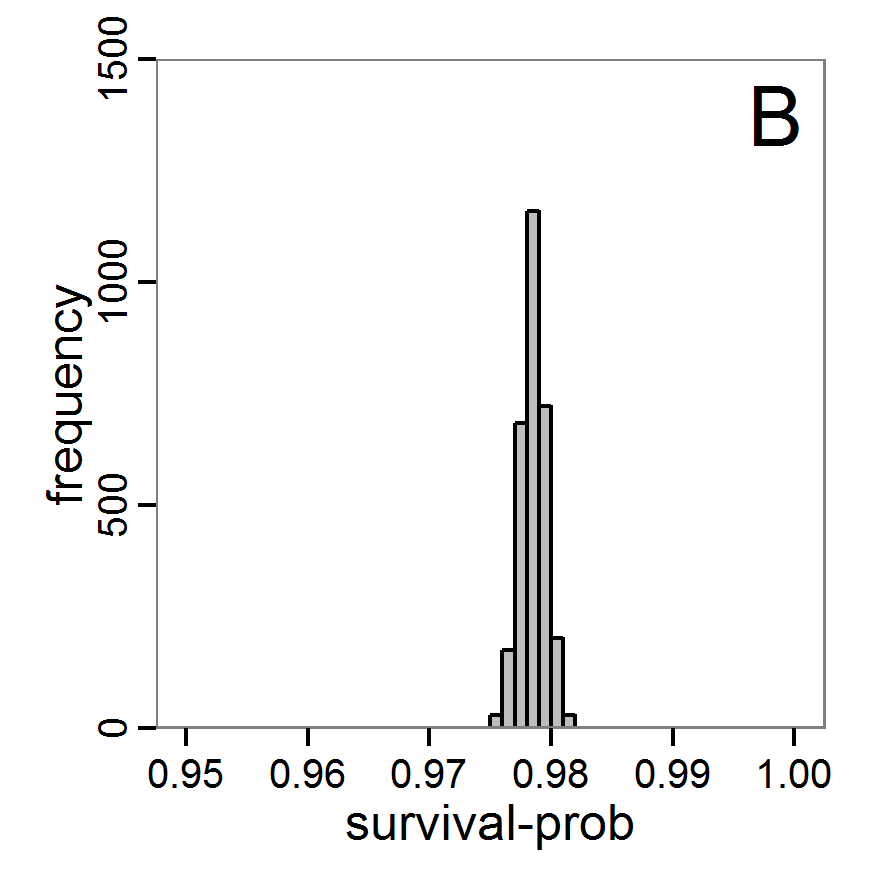
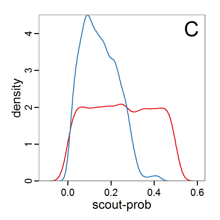
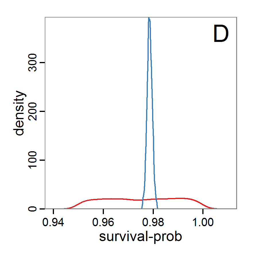
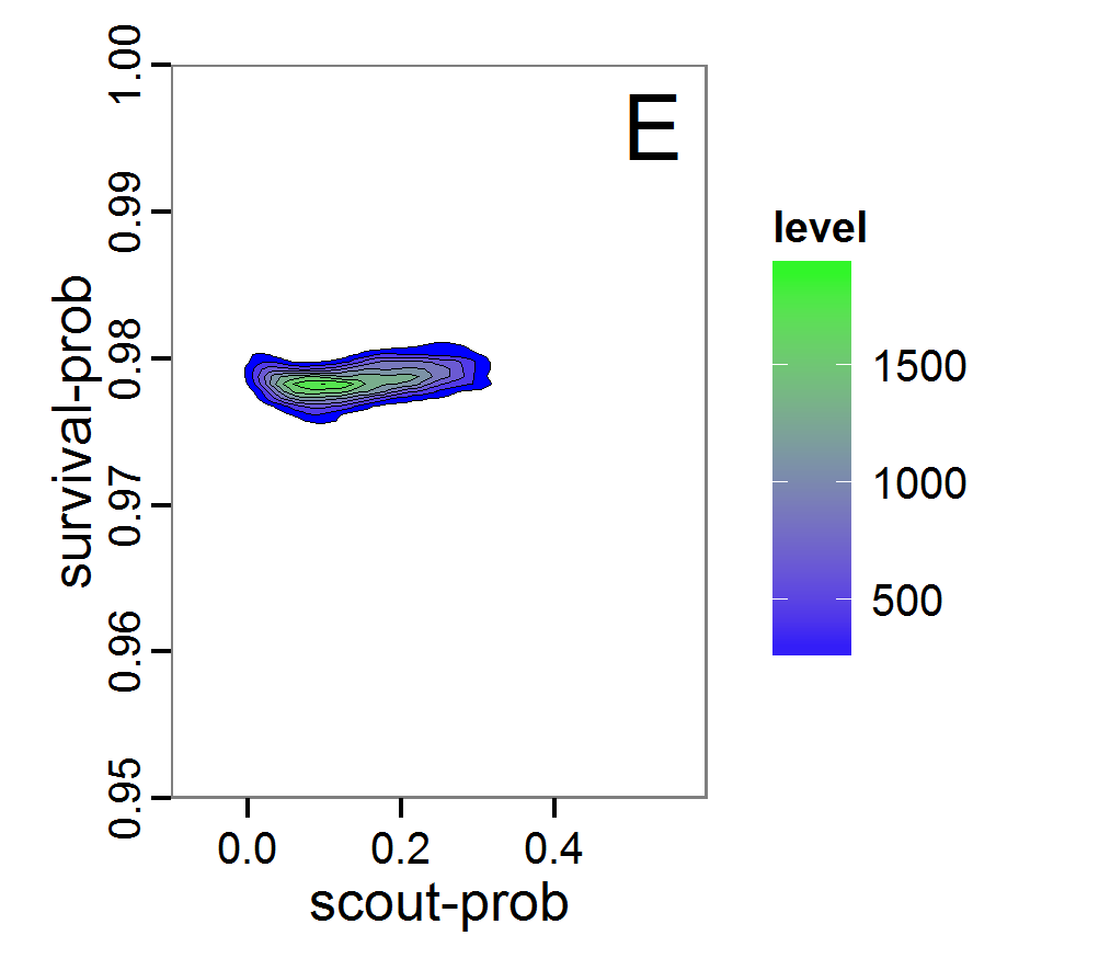
Figure 9. Posterior distribution generated with ABC-MCMC. A: Histogram of accepted runs for scout-prob. B: Histogram of accepted runs for survival-prob. C & D: Density estimation for scout-prob (C) and survival-prob (D) by MCMC sampling (blue line) and from prior distribution (red line). E: joint posterior density estimation of scout-prob and survival-prob by SMC sampling with 10–90% highest density contours. - 2.51
- The results of applying the ABC-MCMC scheme to the example model with a total of 39,991 function calls and 3,000 samples in the posterior distribution are prepared in the same manner as the results of the rejection method and are shown in Figure 9. The results are very similar to those of the rejection sampling method with local linear regression correction but with even narrower posterior distributions. The numerical characteristics of the posterior distributions are processed using the package coda (Plummer et al. 2006) and are given in Table 3.
- 2.52
- The ABC-MCMC scheme is more efficient than rejection sampling, but there are many more fine-tuning possibilities, which can also make its use more complicated.
Table 3: Posterior distribution characteristics for the two parameters gained from the ABC-MCMC algorithm. scout-prob survival-prob Minimum 0.0034 0.9758 5% percentile 0.0280 0.9769 Median 0.1392 0.9785 Mean 0.1474 0.9785 Mode 0.0863 0.9758 95% percentile 0.2840 0.9802 Maximum 0.4296 0.9817 Sequential Monte Carlo
- 2.53
- A sequential Monte Carlo (SMC) method, such as ABC-MCMC, is also used to concentrate the simulations to the zones of the parameter space with high likelihood (Jabot et al. 2013), i.e., to make the sampling more efficient compared to the rejection method. In contrast to MCMC, each step contains not only one parameter set but a sequence of sets (also called a particle or population). A sequence depends on its predecessor, but the simulations within a sequence are independent. The first sequence contains points from the prior distribution and performs a classical rejection algorithm. The successive sequences are then concentrated to those points of the former sequence with the highest likelihood, i.e., points that are nearest to the observed data (Jabot et al. 2013). Therefore, the sequences converge to the posterior distribution based on, in contrast to ABC-MCMC, independent samples. The risk of getting stuck in areas of parameter space that share little support with the posterior distribution is lower than in ABC-MCMC (Hartig et al. 2011). For further reading see Hartig et al. (2011), Jabot et al. (2013) and references therein.
- 2.54
- The EasyABC package (Jabot et al. 2013) for R delivers four variants of SMC. The usage is very similar to the application of ABC-MCMC:
# 1. Define a simulation function (sim) as done for the
# ABC-MCMC method.
# 2. Generate observational summary statistics
# (using the mean of ranges).
obs.sum.stats <- c(abundance=mean(c(115,135)),
variation=mean(c(10,15)),
vacancy=mean(c(0.15,0.3)))
# 3. Generate prior information.
prior <- list('scout-prob'=c("unif",0.0,0.5),
'survival-prob'=c("unif",0.95,1.0))
# 4. Define a sequence of decreasing tolerance thresholds for
# the accepted (normalised) difference between simulated and
# observed summary statistics (in case of multiple summary
# statistics, like here, the deviations are summed and
# compared to the threshold); one value for each step, first
# value for the classical rejection algorithm, last value for
# the max. final difference.
tolerance <- c(1.5,0.5)
# 5. Run SMC.
results.MCMC <- ABC_sequential(method="Beaumont", model=sim,
prior=prior, summary_stat_target=obs.sum.stats,
tolerance_tab=tolerance, nb_simul=20)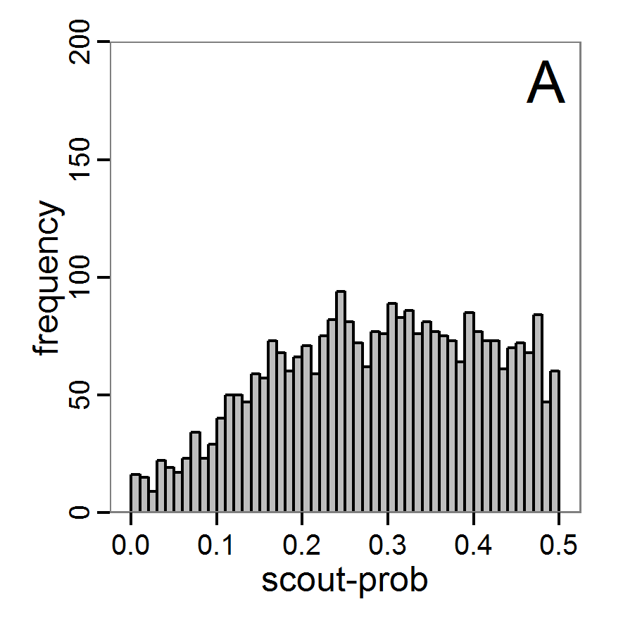
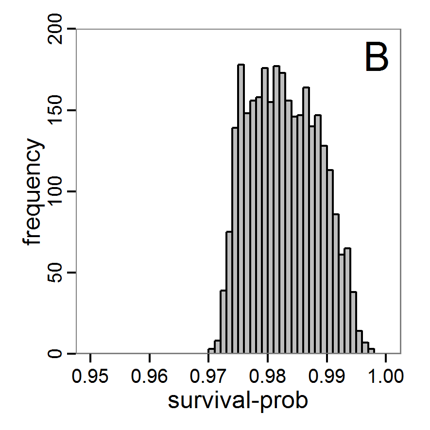
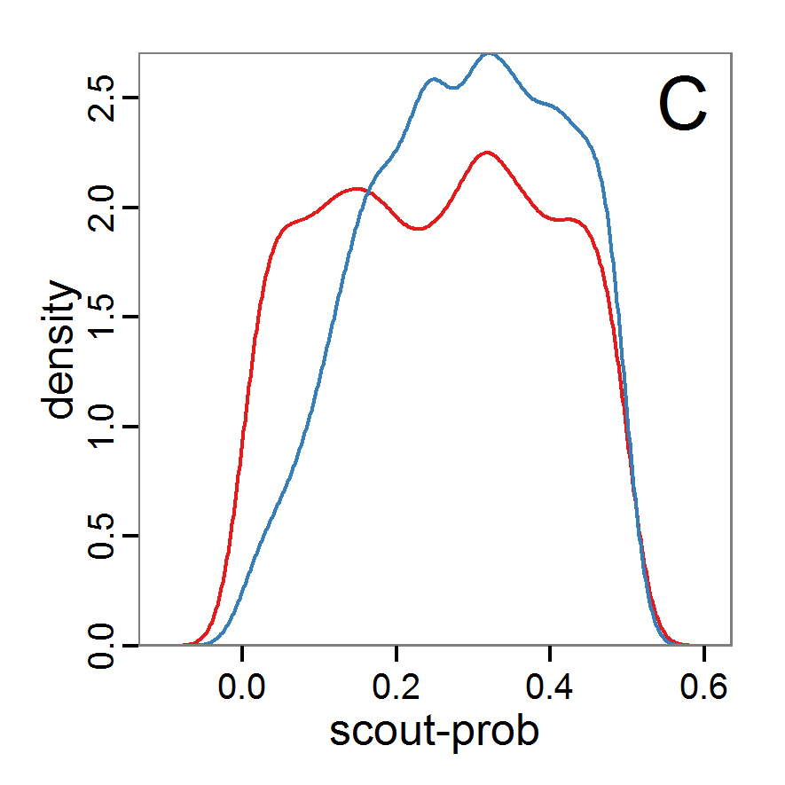
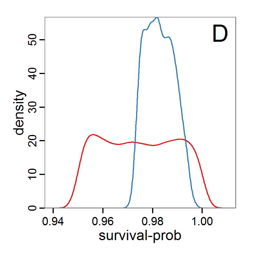
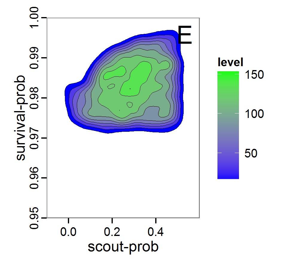
Figure 10. Posterior distribution generated with ABC-SMC. A: Histogram of accepted runs for scout-prob. B: Histogram of accepted runs for survival-prob. C & D: Density estimation for scout-prob (C) and survival-prob (D) by SMC sampling (blue line) and from the prior distribution (red line). E: Joint posterior density estimations of scout-prob and survival-prob by SMC sampling with 10–90% highest density contours. - 2.55
- The results of an application of the ABC-SMC scheme to the example model, prepared in the same manner as for the other ABC schemes, are given in Figure 10 and Table 4. They are based on 11,359 function calls and 3,000 retained samples for the posterior distribution. The distributions share some similarities with the resulting posterior distributions of the other ABC schemes regarding the value range but have different shapes. The posterior distribution of scout-prob does not have its peak at the very small values and is not that different from the prior distribution. The posterior distribution of survival-prob is also broader than with the other schemes. These differences from the other schemes could be the result of the lower sample size, differences in the methodologies, and missing fine-tuning. The multiple fine-tuning options in particular make this method complex for satisfactory application.
Table 4: Posterior distribution characteristics for the two parameters gained from the ABC-SMC algorithm. scout-prob survival-prob Minimum 0.0003 0.9700 5% percentile 0.0785 0.9742 Median 0.2968 0.9825 Mean 0.2852 0.9826 Mode 0.0003 0.9700 95% percentile 0.4741 0.9925 Maximum 0.4999 0.9975 Costs and benefits of approaches to parameter estimation and calibration
- 2.56
- We presented a range of methods for parameter calibration; from sampling techniques over optimisation methods to Approximate Bayesian Computation. Not only the knowledge required to properly apply these methods but also the efficiency of parameter estimation increase in exactly this order. Those modellers who are not willing to become familiar with the details of the more complex methods and are satisfied with less accurate/single parameter values should use the approved Latin hypercube sampling. Those who are interested in very good fits but do not need to worry too much about distributions and confidence bands for the parameter values should take a closer look into the various optimisation methods. The details can become tricky, but methods such as genetic algorithms and simulated annealing are widely used methods with lots of documentation. The ABC methods deliver the most recent approach to parameter calibration but require a much deeper statistical understanding than the other methods as well as sufficient computational power to run a very large number of simulations; on the other hand, these methods deliver much more information than the other methods by constructing a distribution of parameter values rather than one single value. This field is currently quickly evolving, and we see an ongoing development process of new approaches especially designed for the parameterisation of complex dynamic models (e.g.Hartig et al. 2013).
- 2.57
- It is always a good idea to start with a very simple approach, such as Latin hypercube sampling, to acquire a feel for the mechanisms of the model and the response to varying parameter values. From there, one can decide whether more sophisticated methods should be applied to the fitting problem. This sequence avoids the situation in which a sophisticated method is fine tuned first, and it is later realised that the model was not able to produce the observed patterns, requiring a return to model development. Furthermore, it can be interesting to first identify those unknown/uncertain parameters that have a considerable influence on the model results. Then, intensive fine tuning of model parameters can be restricted to the most influential ones. For such an importance ranking, the screening techniques presented in the next section about sensitivity analysis can be of interest.
- 2.58
- As an attempt to rank the methods, we plotted their costs versus the combination of the information generated by the method and the efficiency with which the method generates them (Figure 11). Under costs, we summarised the amount of time one would need to understand the method and to fine-tune its application as well as the computational effort. The most desirable method is the ABC technique, but its costs are much higher than those of the other methods. In the case of large and computationally expensive models, however, the application of ABC techniques may be impossible. Then, the other techniques should be evaluated. For pre-studies, we recommend the application of LHS because it is very simple, can be set up very quickly based on the scripts delivered in the Supplementary Material and can be easily parallelised.
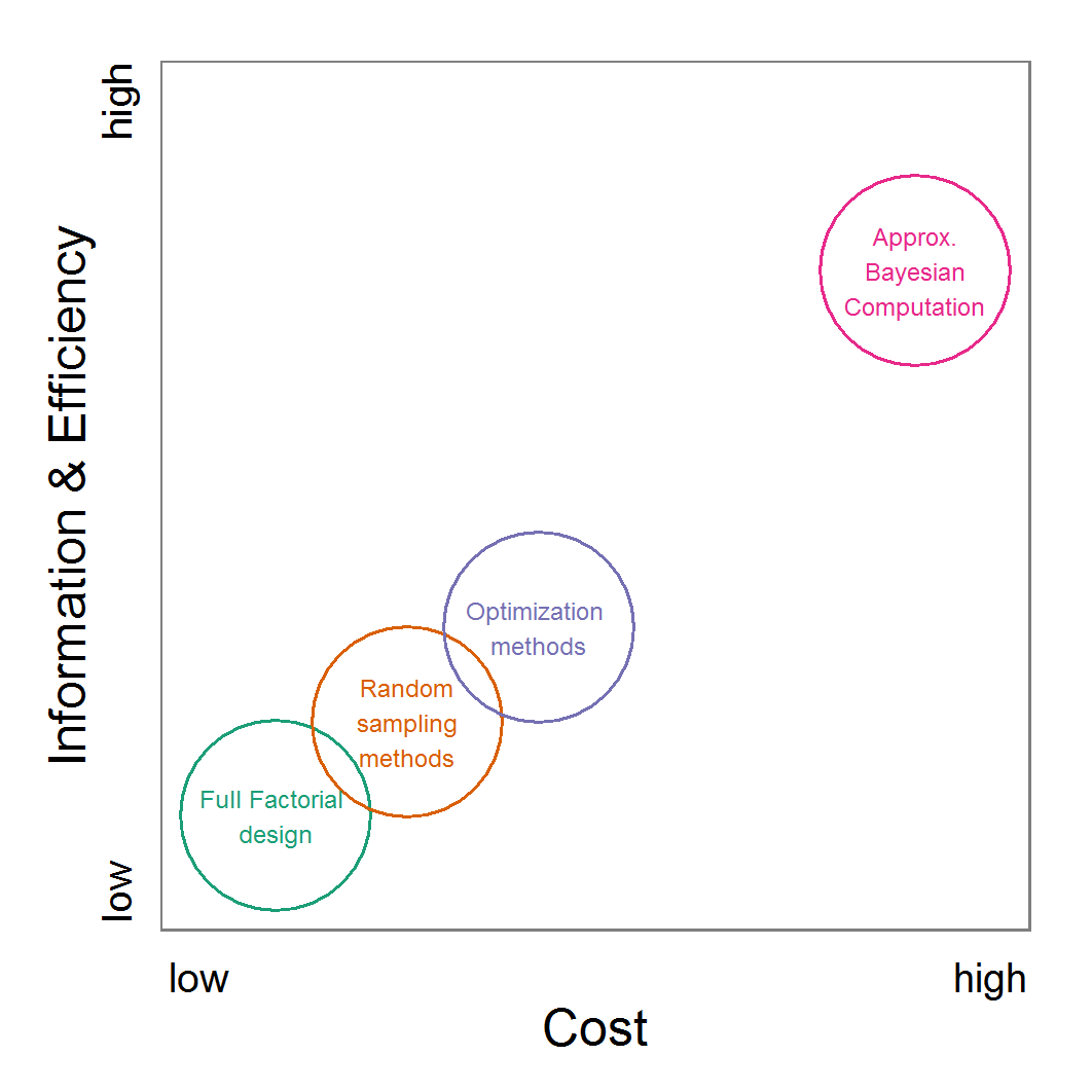
Figure 11. A rough categorisation of the parameter fitting/calibration methods used regarding their cost vs. information and efficiency. Cost includes the computational costs as well as the time required for understanding and fine-tuning the methods. Information and efficiency includes aspects of the type of output and the way to reach it. - 2.59
- For more complex ABMs, runtime might limit the ability to take full advantage of the methods presented here because the models cannot just be run several thousand times. Here, submodels could at least be parameterised independently. For example, in an animal population model, a submodel describing the animals' energy budget could be parameterised independent of the other processes and entities in the full model (e.g., Martin et al. 2013). A limitation of this "divide and conquer" method of parameterisation is that interactions between submodels might in fact exist, which might lead to different parameter values than if the full ABM were parameterised.
Sensitivity analysis
- 3.1
- Sensitivity analysis (SA) is used to explore the influence of varying inputs on the outputs of a simulation model (Ginot et al. 2006). The most commonly analysed inputs are model parameters. SA helps identify those parameters that have a strong influence on model output, which indicates which processes in the model are most important. Moreover, if inputs of the model are uncertain, which is usually the case, sensitivity analysis helps assess the importance of these uncertainties. If the model is robust against variations in the uncertain parameters, i.e., model output does not vary strongly when the parameter values are varied, the uncertainties are of low importance. Otherwise, the parameter values should be well-founded on empirical values (Bar Massada & Carmel 2008; Schmolke et al. 2010). SA is therefore closely related to uncertainty analysis (Ginot et al. 2006). In addition to model parameters, entire groups of parameters, initial values of state variables, or even different model structures can also be considered as inputs to be analysed in SA (Schmolke et al. 2010).
- 3.2
- With sensitivity analysis, three approaches are differentiated: screening, local and global sensitivity analysis (Saltelli 2000; sometimes screening methods are added to global SA methods, see, for example, Cariboni et al. 2007). Screening methods are used to rank input factors by their importance to differentiate between more and less important inputs. These methods are often useful for computationally expensive models because they are very fast in identifying the important parameters, which should be analysed in more detail, but they cannot deliver a quantification of the importance (Saltelli 2000).
- 3.3
- Originating from the analysis of models based on ordinary differential equations, local sensitivity analysis quantifies the effect of small variations in the input factors (Soetaert & Herman 2009; Marino et al. 2008). Classical local sensitivity analysis is often performed as ceteris paribus analysis, i.e., only one factor is changed at a time (the so-called one-factor-at-time approach, OAT) (Bar Massada & Carmel 2008). In contrast, in global sensitivity analysis, input factors are varied over broader ranges. This is of special importance if the inputs are uncertain (Marino et al. 2008), which is mostly the case for ABMs. Furthermore, in global sensitivity analysis several input factors are often varied simultaneously to evaluate not only the effect of one factor at a time but also the interaction effect between inputs; the sensitivity of an input usually depends on the values of the other inputs.
Preliminaries: Experimental setup for the example model
- 3.4
- For simplicity, we will restrict the following examples of sensitivity analyses to three parameters: scout-prob, survival-prob, and scouting-survival. The value ranges and base values used (e.g., for local sensitivity analysis) for the three parameters covered by the sensitivity analysis are listed in Table 5.
- 3.5
- To control stochasticity in the simulation model, we apply the same approach with 10 repeated model runs as described for parameter fitting.
Table 5: Model parameters used in sensitivity analysis. Parameter Description Base value used
by Railsback & Grimm (2012)Base value used here Min. value Max. value scout-prob Probability of undertaking
a scouting trip0.5 0.065 0.0 0.5 survival-prob Probability of a bird
surviving one month0.99 0.978 0.95 1.0 scouting-survival Probability of surviving
a scouting trip0.8 0.8 0.5 1.0 Local sensitivity analysis
- 3.6
- As mentioned above, local sensitivity analysis is often performed as a one-factor-at-time analysis with small variations of the input values. With ABMs, this is often achieved by varying the selected inputs by a specified percentage around their nominal, or default, value. This method provides only limited information regarding model sensitivity, but it is still often used and could be considered a first step in a more detailed analysis when applying a multi-step approach, as proposed, for example, by Railsback et al. (2006). However, when performing such analyses, it should always be kept in mind that interactions between parameters are ignored and that local sensitivities might be completely different if another set of nominal, or default, parameter values were chosen.
- 3.7
- A local sensitivity analysis procedure in R can work in this way:
# 1. Define a simulation function (sim) as done for
# Full factorial design.
# 2. Run simulation using sim function defined in step 1
# for the standard input factor values.
base.param <- c(0.065, 0.978, 0.8)
sim.result.base <- sim(base.param)
# 3. Define a function for changing one of the parameter
# values (here with min and max constraints).
change <- function(i, base, multiplier) {
mod <- base
mod[i] <- min(max(mod[i] * multiplier, 0.0), 1.0)
return(mod)
}
# 4. Create lists of parameter sets with reduced and
# increased parameter values (90% and 110%).
min.params <- lapply(1:length(base.param), change,
base=base.param, multiplier=0.9)
max.params <- lapply(1:length(base.param), change,
base=base.param, multiplier=1.1)
# 5. Run separate simulations (function in step 1) with
# input factor values varied by ±10%.
sim.results <- list()
sim.results$min <- lapply(min.params, sim)
sim.results$max <- lapply(max.params, sim)
# 6. Calculate the deviation between the base model output
# and the outputs using 90% and 110% of the standard value.
dev.min <- sapply(sim.results$min, function(x) {
return((x-sim.result.base)/sim.result.base * 100)})
dev.max <- sapply(sim.results$max, function(x) {
return((x-sim.result.base)/sim.result.base * 100)}) - 3.8
- We selected a variation of 10% for the values, which results, for example, in values for survival-prob of 0.8802 and 1.0 (truncated because the probability cannot exceed 100 per cent). This means that we ran the simulation with three different values of survival-prob: 0.8802, 0.978 and 1.0. To measure the sensitivity of a parameter, we calculate here the change in the output relative to the output with base parameter values. Therefore, we obtain a dimensionless sensitivity measure for all tested parameters that can be easily compared against each other. Of course, there are other sensitivity measures possible. Examples include the calculation of the partial derivative by dividing the change in the output by the change in the parameter value or the calculation of the standard deviation of the output over multiple replications (Railsback & Grimm 2012).
Table 6: Results of a local sensitivity analysis. The columns list the different model outputs and the rows the different input variables (parameters). Values shown are per cent deviations of output values. When changing one parameter, all other parameters are kept constant. Negative output values indicate a reduction of the output value. abundance variation vacancy scout-prob.min -1.0 -6.2 13.7 scout-prob.max 4.0 -8.0 15.4 survival-prob.min -99.9 -97.3 468.6 survival-prob.max 199.0 456.1 -100.0 scouting-survival.min -0.3 -3.7 -1.4 scouting-survival.max 4.9 32.4 -9.8 - 3.9
- Table 6 lists the result of this simple local sensitivity analysis for the example model. It shows that the three outputs are relatively insensitive to small variations in the parameters scout-prob and scouting-survival. In contrast, the model outputs are highly sensitive to variations in parameter survival-prob. However, this conclusion is based on the base values used. Choosing other base values or a different variation percentage could result in completely different conclusions, as the dependence of model output on a single input could be non-linear. Furthermore, we have only learned something about main effects and nothing about the interaction effects when two or more inputs are varied at the same time.
Screening methods
- 3.10
- Screening methods try to answer the question which of a large set of potentially important inputs actually have a strong influence on the simulation output of interest. They are designed to be computationally efficient and able to explore a large set of inputs. Often, one-factor-at-time approaches are applied but, in contrast to local sensitivity analysis, with variations of the inputs over a wide range of values (Campolongo, Saltelli et al. 2000). We restrict ourselves here to Morris's elementary effects screening, which appears to be the most important suitable method for ABMs. Other well-known methods are often not suitable for ABMs. For example, to use Bettonvil's sequential bifurcation, available in package sensitivity (Pujol et al. 2012), the user needs to know the sign of the main effects of all tested parameters in advance, which often cannot be logically deduced in ABMs, as the relationships between parameter values and model outputs are complex and non-linear.
Morris's elementary effects screening
- 3.11
- The Morris method was developed to explore the importance of a large number of input factors in computer models that cannot be analysed by classical mathematical methods (Morris 1991). Furthermore, the method is free of assumptions about the model, for example, the signs of effects (Saltelli et al. 2004). Based on individually randomised one-factor-at-a-time designs, it estimates the effects of changes in the input factor levels, i.e., the parameter values, which are called elementary effects (EEs). The EEs are statistically analysed to measure their relative importance. The results of the Morris method are two measures for every investigated input factor: μ, the mean of the elementary effects, as an estimate of the overall influence of an input factor/parameter, and σ, the standard deviation of the elementary effects, as an estimate of higher order effects, i.e., non-linear and/or interaction effects (Campolongo et al. 2007). Still, this method does not identify interactions between specific input factors but instead delivers only lumped information about the interaction effect of one factor with the rest of the model (Campolongo, Kleijnen et al. 2000). Examples for the application of the Morris screening method in the context of ABM can be found in Imron et al. (Imron 2012), Vinatier et al. (2013), and Vinatier, Tixier et al. (2009).
- 3.12
- The Morris screening method is available in R through the sensitivity package (Pujol et al. 2012). The function morris includes the Morris method with improvements in sampling strategy and the calculation of μ* to avoid Type-II errors (Campolongo et al. 2007). When positive and negative effects occur at different factor levels, they can cancel each other out in the calculation of μ, whereas μ* can handle this case. The application of the morris function in R can be performed as follows:
# 1. Define a simulation function (sim) as done for
# Full factorial design.
# 2. Create an instance of the class morris and define min
# (referred to as binf) and max (bsup) values of the
# parameters to be tested, the sampling design (design, here
# oat = Morris One-At-a-Time design with 5 levels), and the
# number of repetitions of the design (r).
mo <- morris(model = NULL, factors = 3, r = 4,
design = list(type = "oat", levels = 5,
grid.jump = 3), binf = c(0.0, 0.95, 0.5),
bsup = c(0.5, 1.0, 1.0), scale=TRUE)
# 3. Get simulation model responses for sampling points using
# the sim function defined in step 1.
sim.results <- apply(mo$x, 1, sim)
# 4. Add simulation results to the morris object.
tell(mo, sim.results) - 3.13
- For the interpretation of the results, Saltelli et al. (2004) recommend comparing the values of σ and μ, or better μ*. High values of μ indicate that a factor has an important overall influence on the output and that this effect always has the same sign (Saltelli et al. 2004). In contrast, when there is a high value of μ* and a low value of μ, it indicates that there is a non-monotonic effect on the output. High values of σ indicate that the elementary effects strongly depend on the choice of the other input factors, whereas a high μ or μ* and a low σ indicate that the elementary effect is almost independent of the values of the other factors, which means that it is a first-order/main effect. In summary, the Morris screening method delivers measures of relative importance but cannot quantify the strength of the effects.
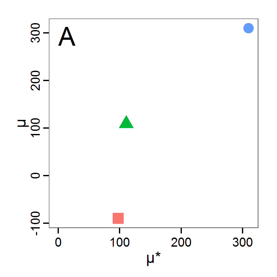
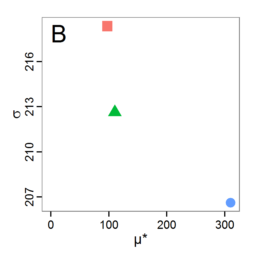
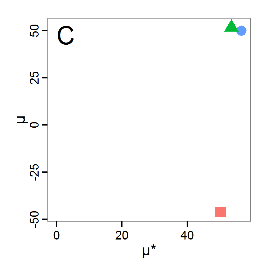
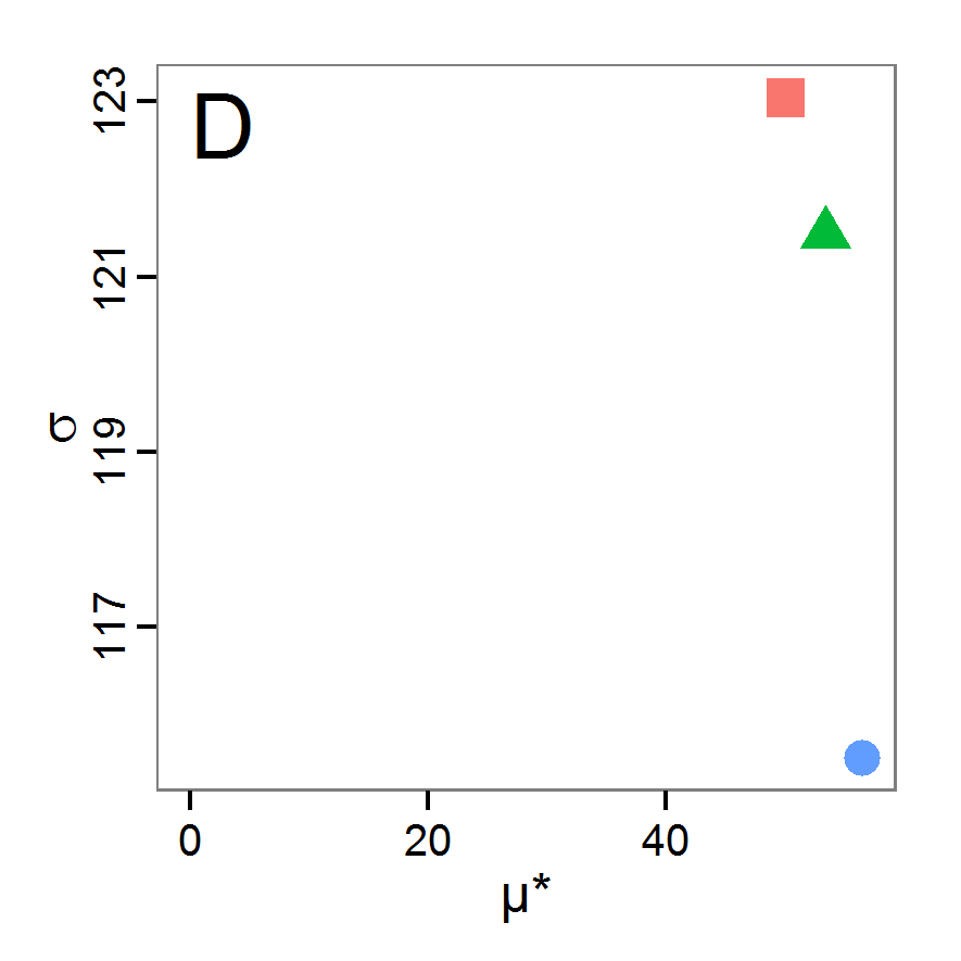
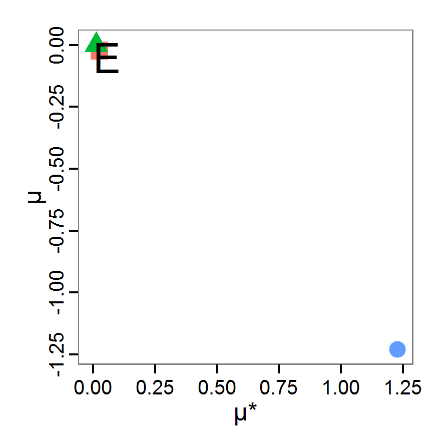
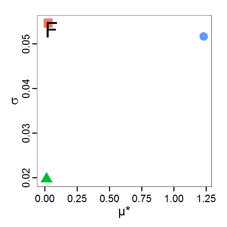
Figure 12. Results of the Morris screening method. Red rectangle: scout-prob, blue point: survival-prob, green triangle: scouting-survival. A: Test for overall importance (high μ) and non-monotonic relationship (low μ and high μ*) for the abundance output. B: Test for interaction (high σ) and main effect (high μ* and low σ) for the abundance output. C: same as A for variation output. D: same as B for variation output. E: same as A for vacancy output. D: same as B for vacancy output. - 3.14
- The results of an application of the Morris screening method to our example model with 40 function calls is shown in Figure 12. The plots on the left side (panels A, C, and E) indicate high overall influences of survival-prob for all three outputs, the abundance, variation, and vacancy criteria. The other two factors, scout-prob and scouting-survival, have a less important influence, but still are influential, on the abundance output (panel A). On the variation output (panel C), all three input factors are of nearly the same importance, and no clear importance ranking can be performed. From panel E, we learn that the other two factors, scout-prob and scouting-survival, are irrelevant for the vacancy output. Moreover, in panel A we see that the absolute values of μ and μ* are the same for scout-prob but with a negative sign for μ. This leads to the conclusion that the influence of scout-prob on the abundance output is monotonic but negative. The same also applies to the variation output and to the influence of survival-prob on the vacancy output. No case of low μ but high μ* value can be found; therefore, we can conclude that all effects are mostly monotonic. Panels B, D, and F deliver information about non-linear and/or interaction effects. Because all three factors are important for the abundance and variation outputs, we should check all three of these factors for non-linear/interaction effects. Panel B shows that the values of σ are highest for scout-prob and scouting-survival, although their μ* values are relatively low. This leads to the conclusion that the influence of these two factors on the abundance output is strongly non-linear and/or dependent on the values of the other factors. Although the σ value for survival-prob is relatively low, compared to the other factors, it remains high (~66% of μ*). This means that there is also an interaction and/or non-linear effect of survival-prob on the abundance output, but with a lower contribution to the overall influence relative to the other two factors. From the variation output in panel D we see that there is a very strong interaction/non-linear effect for scout-prob and scouting-survival and a lesser, but still very strong, interaction/non-linear effect detected for survival-prob. For the vacancy output, we do not have to interpret the σ values for scout-prob and scouting-survival because these factors have been identified as unimportant. For survival-prob, the only important factor for the vacancy output, the σ value is low (approx. 4% of μ*). Therefore, we can conclude that it is mostly a main-/first-order effect.
- 3.15
- Overall, we learned a great deal about the example model by applying the Morris screening method. Furthermore, a graphical analysis of the relationship between μ* and μ as well as between μ* and σ is simple but very useful. If one is only interested in ranking the input factors by their importance, a comparison of the values of μ* should be sufficient.
Global sensitivity analysis
- 3.16
- In global sensitivity analysis, input variables are varied over the full range of their possible values. This distinguishes these methods from local sensitivity analysis. Moreover, in global sensitivity analysis effects are quantified, which is different from screening methods, which deliver only a ranking of the input variables by their importance for the output without quantification.
- 3.17
- For some methods described below, such as partial correlation coefficients, it can be useful to perform a graphical analysis first to obtain a basic idea of the relationships between inputs and outputs. For such graphical analyses, for example, scatter and interaction plots, full factorial design and Latin hypercube sampling can be appropriate.
Excursion: Design of Experiment
- 3.18
- The Design of Experiment (DoE) methodology, which was first formulated for experiments in agriculture (Lorscheid et al. 2012), can be used for sensitivity analysis. Introductions to the application of classical DoE for ABMs can be found, for example, in Campolongo and Saltelli (2000), Happe (2005), or Lorscheid et al. (2012).
- 3.19
- As a first step, an experimental design must be selected. For simplicity, we use a full factorial design of the two extreme values of each of the k inputs (2k, i.e., eight function calls for the example), which has also been used by Lorscheid et al. (2012) and Happe (2005). Then, we run the simulation for the design points, i.e., parameter sets, and add the (averaged, in the case of stochastic models) simulation results to the so-called design matrix. This procedure can be run using package FrF2 (Groemping 2011) or DoE.base (Groemping 2013b) and could look like this:
# 1. Define a function that runs the simulation model
# for a given input factor combination and returns the
# simulation output (averaged) as well as the output of
# each iteration into anova.df in case of repeated
# simulations for stochastic models.
# See Supplementary Material (simulation_function5.R) for an
# implementation example using RNetLogo.
sim <- function(input, anova.df.name=="anova.df") {
...
return(output)
}
# 2. Create full factorial design (2^k, i.e., k = number of
# parameters; therefore, only extreme values are tested).
ff <- FrF2(nruns=2^3, nfactors=3, randomize=False,
factor.names=c('scout-prob',
'survival-prob',
'scouting-survival'))
# 3. Get simulation model response (sim.results and
# anova.df) for sampling points (ff) using sim function
# defined in step 1.
anova.df <- data.frame()
sim.results <- apply(as.data.frame(ff), 1, sim,
anova.df.name="anova.df")
# 4. Add simulation model response to the design matrix.
ffr <- add.response(ff, response=sim.results) - 3.20
- Happe (2005) analysed the results by fitting a linear regression model (so-called metamodel) with the simulation inputs as independent variables and the simulation output as a dependent variable. Not performed by Happe (2005), but also known in DoE, is the usage of the metamodel to predict the results of input value combinations that have not been simulated (look for a predict function for the method you used to produce the metamodel in R). Non-parametric alternatives to linear or non-linear regression models for prediction as recommended by Helton et al. (2006) are generalised additive models (GAM, see R package gam,Hastie 2011), locally weighted regression (LOESS, see function loess in R's base package) and projection pursuit regression (function ppr in R's base package). For example, GAM was used by Han et al. (2012) for analysing a complex, stochastic functional-structural fruit tree model. Kriging, a geostatistical method, has also been applied for metamodel construction in ABMs; see, for example, Salle & Yidizoglu (2012). Kriging methods are available in several R packages, see, for example, DiceEval (Dupuy & Helbert 2011), kriging (Olmedo 2011), or RandomFields (Schlather et al. 2013). The approach of using metamodels to predict the model output of non-simulated input factor combinations is strongly related to the response surface method (RSM, see R package rsm, Lenth 2009) (Ascough Il et al. 2005).
- 3.21
- The procedure described in Happe (2005) can be realised in R as follows:
# 5. Create effect plots.
MEPlot(ffr)
IAPlot(ffr)
# 6. Perform stepwise fitting of a (linear) regression model
# to the data of step 4 (stepAIC requires package MASS,
# Venables & Ripley 2002).
in.design <- cbind(as.data.frame(ff), sim.results)
min.model <- lm(abundance ~ scout_prob, data=in.design)
max.model <- lm(abundance ~ scout_prob * survival_prob *
scouting_survival, data=in.design)
lms <- stepAIC(min.model, scope=list(lower=min.model,
upper=max.model))
- 3.22
- The resulting main effect and two-way interaction effect plots are shown in Figures 13 and 14, respectively. The strongest main effects for all outputs are detected for the input factor survival-prob, with positive signs for abundance and variation and a negative sign for the vacancy output. For the two other input factors, no main effects for the vacancy output and a small one for the other two outputs were detected, with negative signs for scout-prob and positive signs for scouting-survival. The two-way interaction effect plots indicate interaction effects if the lines for a factor combination are not parallel. The less parallel the lines are, the higher is the expected interaction effect. We see interaction effects for all factor combinations for the abundance and the variation outputs but no two-way interaction effects for the vacancy output. These results are in accordance with the results from the Morris screening method.
- 3.23
- Looking at Table 7, we see the results of a stepwise linear regression fitting (metamodelling). Survival-prob was retained in all three of the final regression models for the different outputs and was statistically significant (see column Pr(>|t|)). Furthermore, the sign of the estimate for survival-prob is in accordance with the visual findings. The other main effects found in the visual detection have not been retained in or added to the metamodel because they were not able to improve the model regarding the Akaike information criterion (AIC). In contrast, the main effect of scouting-survival has been added to the metamodel for the vacancy output, which was not detected in the visual analysis. However, this predictive variable has no statistically significant effect on the metamodel and should therefore be removed in a further step.
- 3.24
- Our visual findings about the interaction effects have not been selected for the metamodel by the stepwise regression fitting. Only for the vacancy output has the interaction effect between survival-prob and scouting-survival been included, but this effect also has no significant effect on the metamodel but just improves the AIC. Therefore, it should be removed. These results can strongly depend on the selection measure used - here AIC, but R2 and others are also possible – and on the direction of the stepwise search, here "forward" selection.
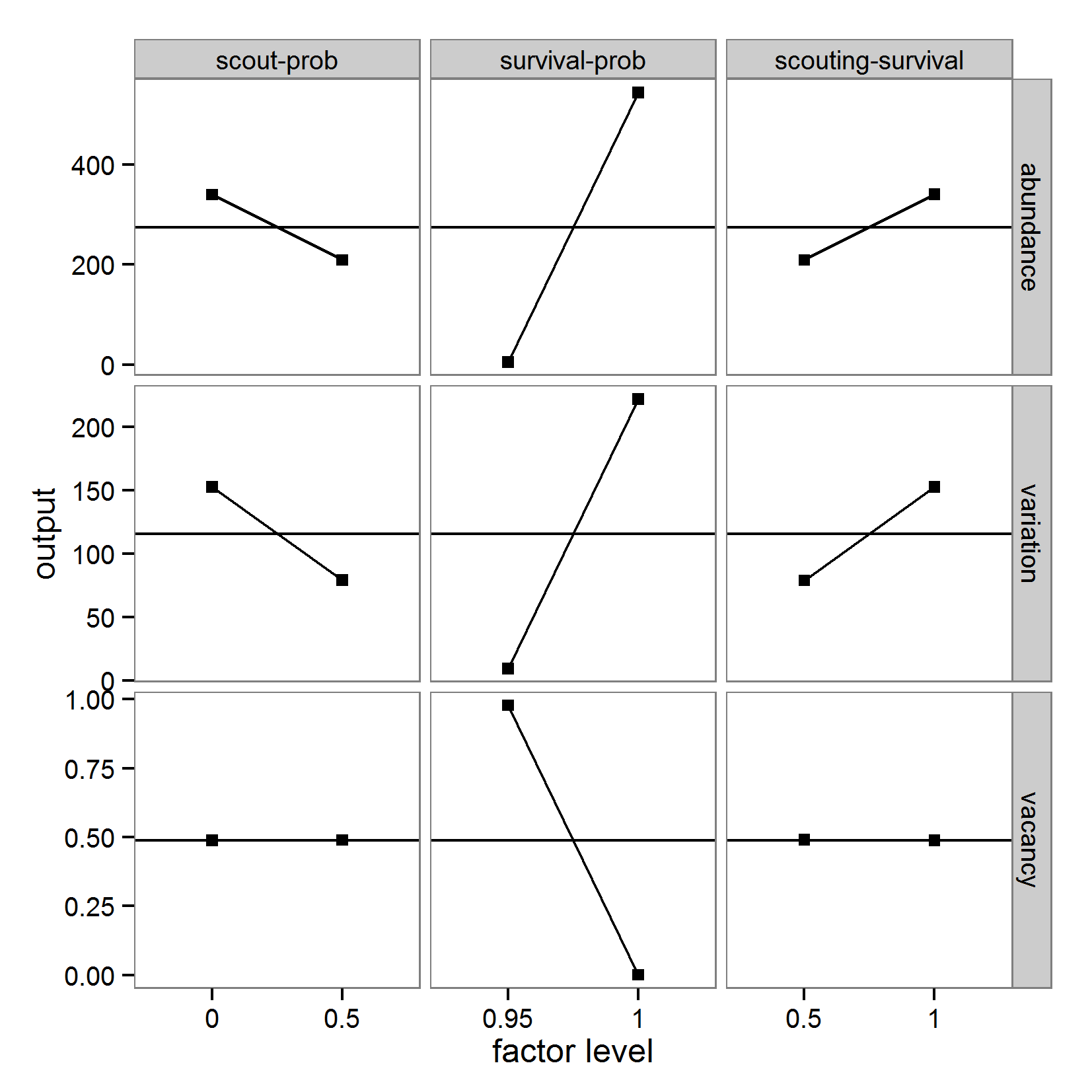
Figure 13. Main effect plots (based on linear regression model). Parameters in columns (left: scout-prob, middle: survival-prob, right: scouting-survival) and outputs in rows (top: abundance, middle: variation, bottom: vacancy). Horizontal lines (without rectangles) in rows visualise mean values. Right rectangle higher than left rectangle indicates a main effect with a positive sign and vice versa. Rectangles on the same output value (y-axis) indicate no main effect. 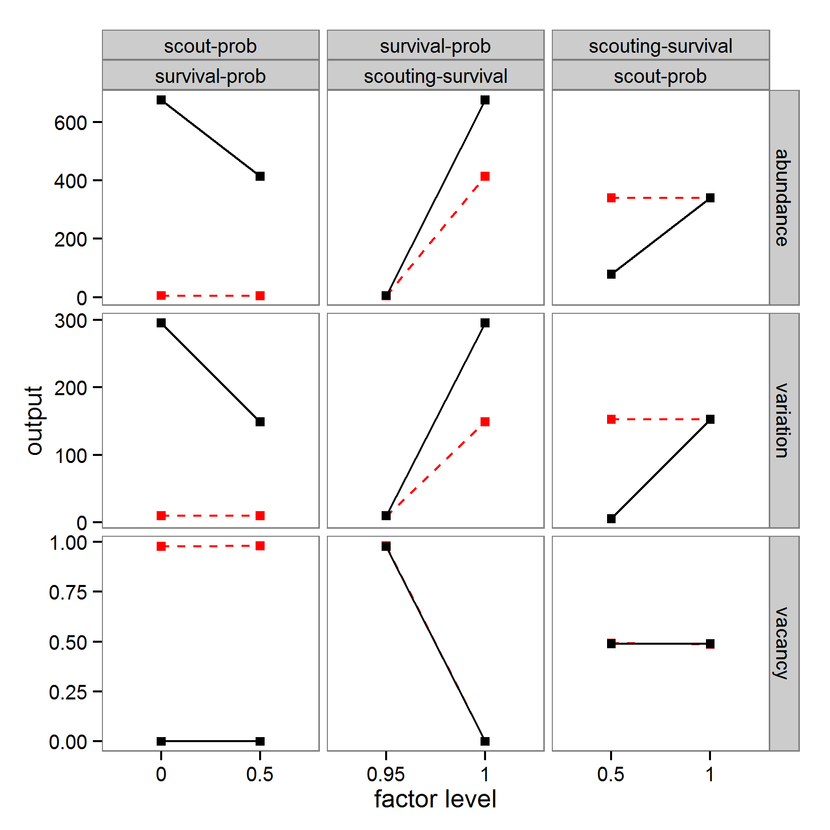
Figure 14. Interaction effect plots (based on linear regression). Left column: scout-prob interacting with survival-prob. Red dotted line: value of survival-prob is 0.95, black solid line: value of survival-prob is 1.0. Middle column: survival-prob interacting with scouting-survival. Red dotted line: value of scouting-survival is 0.5, black solid line: value of scouting-survival is 1.0. Left column: scouting-survival interacting with scout-prob. Red dotted line: value of scout-prob is 0.0, black solid line: value of scout-prob is 0.5. Output in rows (top: abundance, middle: variation, bottom: vacancy). Lines in parallel indicate no interaction effect. Table 7: Results of a stepwise linear regression fitting based on 2k-design. Names in the first column are the input factors. Single names are main effects. Names combined with a colon are interaction effects. Estimate Std. Error t-Value Pr(>|t|) a) abundance output Final Model: abundance ~ survival-prob (adj. R2: 0.6958) Intercept -10238 2550 -4.02 0.00699 ** survival-prob 10783 2614 4.13 0.00618 ** b) variation output Final Model: variation ∼ survival-prob (adj. R2: 0.5127) Intercept -4034 1436 -2.81 0.0307 * survival-prob 4257 1472 2.89 0.0276 * c) vacancy output Final Model: vacancy ∼ survival-prob + scouting-survival +
survival-prob:scouting-survival (adj. R2: 1.0)Intercept 19.70 0.09 230.31 2.13e-09 *** survival-prob -19.70 0.09 -224.63 2.36e-09 *** scouting-survival -0.20 0.11 -1.81 0.14 survival-prob:scouting-survival 0.20 0.11 1.77 0.15 - 3.25
- An alternative approach to that used by Happe (2005) was used by Lorscheid et al. (2012). They calculated an effect matrix that delivers a description of the main and interaction effects. In a preliminary step, the results of all simulations (data.frame anova.df of step 3 in the R code above) are analysed for significant main and interaction effects using an ANOVA (or non-parametric substitute). If needed, this process can be run iteratively as a "cascaded DoE" for complex inputs, i.e., factors that represent several sub-factors, as described in Lorscheid et al. (2012). A non-iterative procedure, which could be easily adapted to an iterative one, can be realised in R as follows (steps 1-4 correspond to the previous R code example):
# 5. Calculate ANOVA with anova.df data.frame from step 3
glm(formula = output ~ scout_prob * survival_prob *
scout_survival, data=anova.df)
# 6. Define a function that calculates the effects between
# parameters after Saltelli et al. (2000) as follows:
#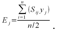
# 7. Calculate main and interaction effects using the
# function defined in step 6 and data in ffr from step 4 up
# to the desired interaction level. Use desnum(ffr) to obtain
# the level signs needed for the effect calculation. See
# Supplementary Materials (SM14b_DoE_effect_matrix.R) for an
# implementation example.Table 8: Results of the ANOVA. Signif. codes: '***' 0.001 '**' 0.01 '*' 0.05. Names in the first column are the input factors. Single names are main effects. Names combined with a colon are interaction effects. Df Sum Sq. Mean Sq. F value Pr(>|t|) 1) abundance output scout-prob 1 342330 342330 309953 < 2e-16 *** survival-prob 1 5813439 5813439 5263611 < 2e-16 *** scouting-survival 1 343050 343050 310604 < 2e-16 *** scout-prob:survival-prob 1 341010 341010 308757 < 2e-16 *** scout-prob:scouting-survival 1 341153 341153 308887 < 2e-16 *** survival-prob:scouting-survival 1 340292 340292 308107 < 2e-16 *** scout-prob:survival-prob:
scouting-survival1 342186 342186 309822 < 2e-16 *** Residuals 72 80 1 2) variation output scout-prob 1 108419 108419 52704 < 2e-16 *** survival-prob 1 905960 905960 440401 < 2e-16 *** scouting-survival 1 109103 109103 53036 < 2e-16 *** scout-prob:survival-prob 1 108228 108228 52611 < 2e-16 *** scout-prob:scouting-survival 1 108216 108216 52606 < 2e-16 *** survival-prob:scouting-survival 1 107547 107547 52280 < 2e-16 *** scout-prob:survival-prob:
scouting-survival1 108430 108430 52710 < 2e-16 *** Residuals 72 148 2 3) vacancy output scout-prob 1 0 0 1.03e-1 0.749 survival-prob 1 19.11 19.11 2.33e+5 < 2e-16 *** scouting-survival 1 0 0 1.46e-1 0.231 scout-prob:survival-prob 1 0 0 1.03e-2 0.749 scout-prob:scouting-survival 1 0 0 8-33e-1 0.364 survival-prob:scouting-survival 1 0 0 1.46e-1 0.231 scout-prob:survival-prob:
scouting-survival1 0 0 8.33e-1 0.364 Residuals 72 0.006 0 - 3.26
- The results of the ANOVA for the identification of significant effects are given in Table 8. For the abundance and variation outputs, all terms are highly significant, whereas only the input factor survival-prob is significant for the vacancy output.
Table 9: DoE main/first-order and second-order effect matrix. scout-prob survival-prob scouting-survival 1) abundance scout-prob -130.830 -130.578 130.605 survival-prob 539.140 130.440 scouting-survival 130.968 2) variation scout-prob -73.627 -73.562 73.558 survival-prob 212.833 73.330 scouting-survival 73.859 3) vacancy scout-prob 0.0007 -0.0007 0.0019 survival-prob -0.9776 0.0025 scouting-survival -0.0025 - 3.27
- When comparing the ANOVA results (Table 8) with the effect matrix (Table 9, calculated in step 7 of the R code sample above), we see that the findings from the ANOVA correspond to the values in the effect matrix, i.e., we find high main effect values (on the diagonal of each sub-matrix) for the abundance and variation outputs for all parameters, and for vacancy, a considerable effect (with negative sign) only for the main effect of survival-prob. The main effect of scout-prob and the interaction between scout-prob and survival-prob have negative signs for the abundance and variation outputs, whereas the other effects have positive signs. These findings correspond to the main and interaction plots based on linear regressions from the previous method.
- 3.28
- A 2k -design, as used by Happe (2005) and Lorscheid et al. (2012), will only be appropriate for linear and monotonic relationships between inputs and outputs. Of course, different sampling designs with space-filling curves like Latin hypercube sampling (LHS) could be applied, and in case of metamodelling, non-linear regression models, splines, neural networks or Kriging methods can be used (Siebertz et al. 2010). However, methods that build on the fundamentals of DoE and were especially developed for sensitivity analysis are already available and more efficient. For non-linear and non-monotonic responses, see, for example, the Sobol' method (see below) as an adaption of DoE principles to computational experiments. Nevertheless, the adapted DoE methods presented here are relatively easy to understand and communicate and do not require extensive computations (depending on the sampling scheme). Therefore, if the model characteristics fit the methods' requirements, they can be used for a quick but still useful first global sensitivity analysis.
Regression-based methods
Partial (rank) correlation coefficient
- 3.29
- Correlation techniques measure the strength of a linear relationship between an input and an output variable. Partial correlation techniques enable the user to measure the strength of the relationship of more than one input variable (Campolongo, Saltelli et al. 2000). Therefore, if linear relationships are expected, the partial correlation coefficient (PCC) can be applied as a sensitivity measure. Instead, if non-linear but monotonic associations are expected, partial rank correlation coefficients (PRCC) are used to measure the strength of the relationship. Both methods are robust measures as long as input factors are uncorrelated (Marino et al. 2008). An example of the application of PRCC to an ABM can be found in Marino et al. (2008).
- 3.30
- For both PCC and PRCC, a sample of model outputs must be created first. It is preferable to use a Latin hypercube sampling (LHS) scheme (Blower & Dowlatabadi 1994), but other sampling schemes could also be applied. Both PCC and PRCC are implemented in the sensitivity package for R (Pujol et al. 2012). Therefore, calculating the PCC/PRCC in R can look like this:
# 1. Define a simulation function (sim) as done for
# Full factorial design.
# 2. Create parameter samples from, for example, a uniform
# distribution using function lhs from package tgp
# (Gramacy & Taddy 2013).
param.sets <- lhs(n=100, rect=matrix(c(0.0,0.95,0.5,1.0), 2))
# 3. Iterate through the parameter combinations from step 2
# and call function sim from step 1 for each parameter
# combination.
sim.results <- apply(as.data.frame(param.sets), 1, sim)
# 4. Calculate the partial (rank) correlation coefficient
# based on the simulation results of step 3.
pcc.result <- pcc(x=param.sets, y=sim.results, nboot = 100,
rank = FALSE) - 3.31
- The result of an application of PCC/PRCC on the example model with 200 samples is shown in Figure 15. Obviously, there is a very strong positive linear relationship between the survival-prob input factor and the abundance output as well as a strong negative linear relationship between the same input factor and the vacancy output. Because the (absolute) values for the PRCC for scout-prob and scouting-survival in panel C are greater than for PCC, this could indicate a non-linear but monotonic relationship between these two factors and the vacancy output. For the abundance output (panel A), there is a weak linear relationship detected for the input factors scout-prob (with a negative sign) and scouting-survival (with a positive sign). For the variation output (panel B) there is no obvious importance ranking. Either there is only a small influence of the input factors on the output, the relationship is non-monotonic or the input factors are not independent (which is actually the case, as we will see later using variance decomposition).
- 3.32
- In summary, the PCC and especially the PRCC are often used as importance measures. They are relatively easy to understand, interpret and communicate and are a quantitative alternative to qualitative, visual sensitivity analysis using, for example, scatterplots (Hamby 1995).
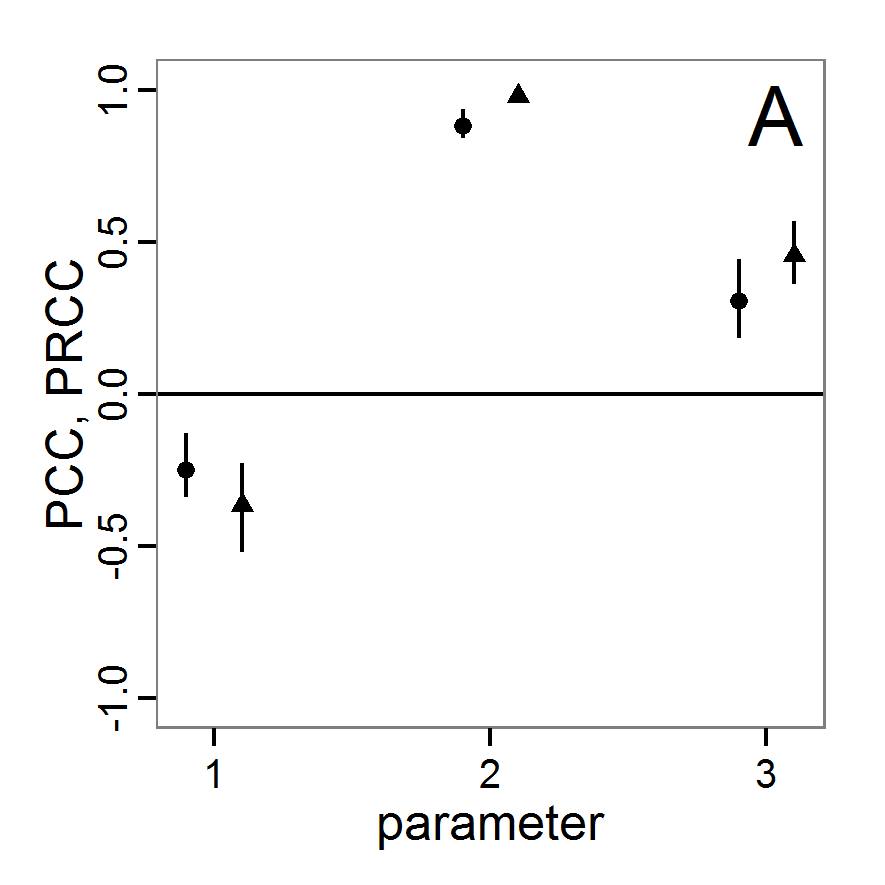
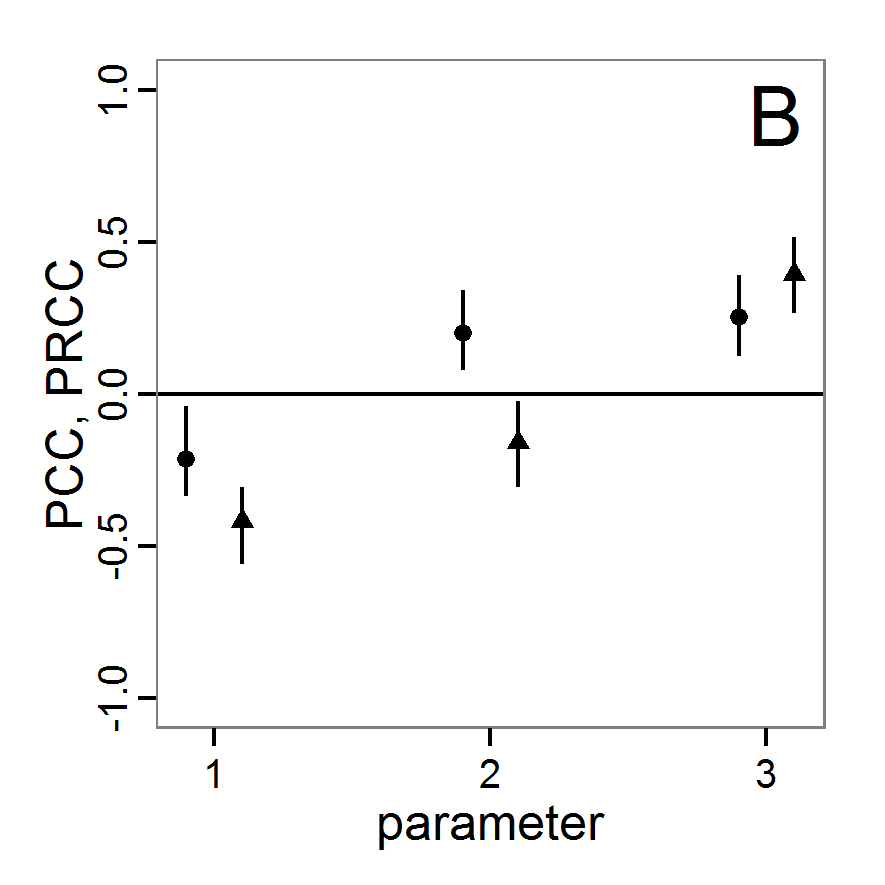
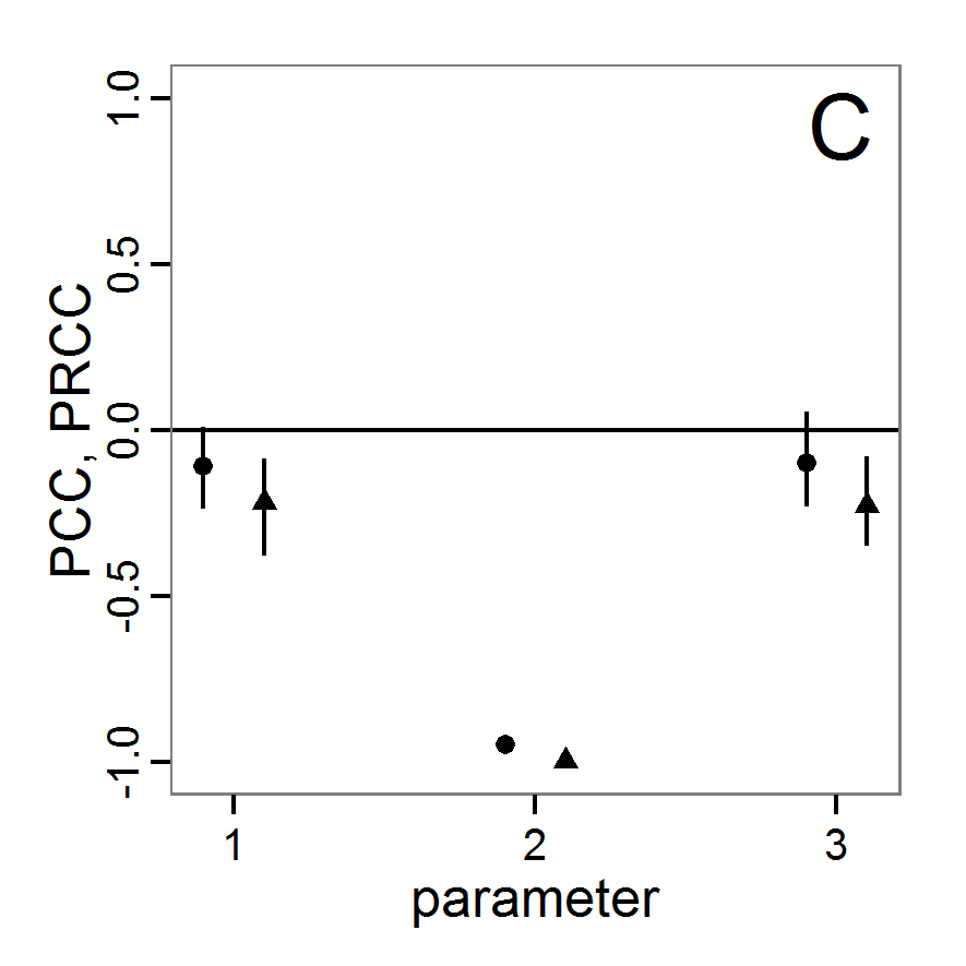
Figure 15. Results of the PCC/PRCC. A: for abundance output. B: for variation output. C: for vacancy output. Circles (to the left of each x-axis tick) show original PCC values (measure of linear relationship). Triangles (to the right of each x-axis tick) show original PRCC values (measure of linear or non-linear but monotonic relationship). Sticks show bootstrapped 95% confidence intervals of corresponding sensitivity indices. Numbers on x-axis for all plots: 1: scout-prob, 2: survival-prob, 3: scouting-survival. Standardised (rank) regression coefficient
- 3.33
- The methods of standardised regression coefficient (SRC) and standardised rank regression coefficient (SRRC) deliver similar results to those of PCC/PRCC but are more strongly influenced by the distribution from which the tested parameter values are drawn (Campolongo, Saltelli et al. 2000). In a first step, fitting a linear regression model to the simulation data delivers measures of the relationship between the inputs and output of the simulation model. The regression coefficients are standardised by multiplication with the ratio between standard deviations of input factor and output value. In SRRC, the original values are replaced by ranks. As with PCC and PRCC, SRC is only able to measure linear relationships, whereas SRRC can also be used for non-linear but monotonic associations between input and output variables when little or no correlation between the input factors exists (Marino et al. 2008).
- 3.34
- These methods are also implemented in the sensitivity package for R (Pujol et al. 2012), and the application is equivalent to that of PCC/PRCC (therefore not shown here; see PCC/PRCC and replace the function call pcc with src).
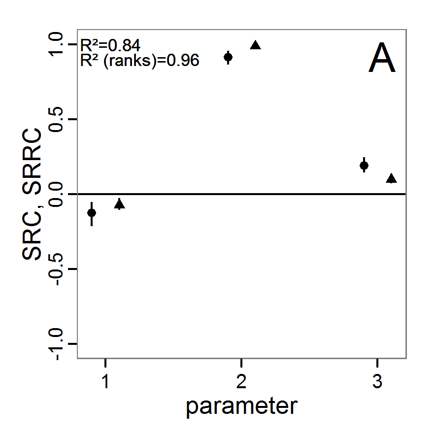
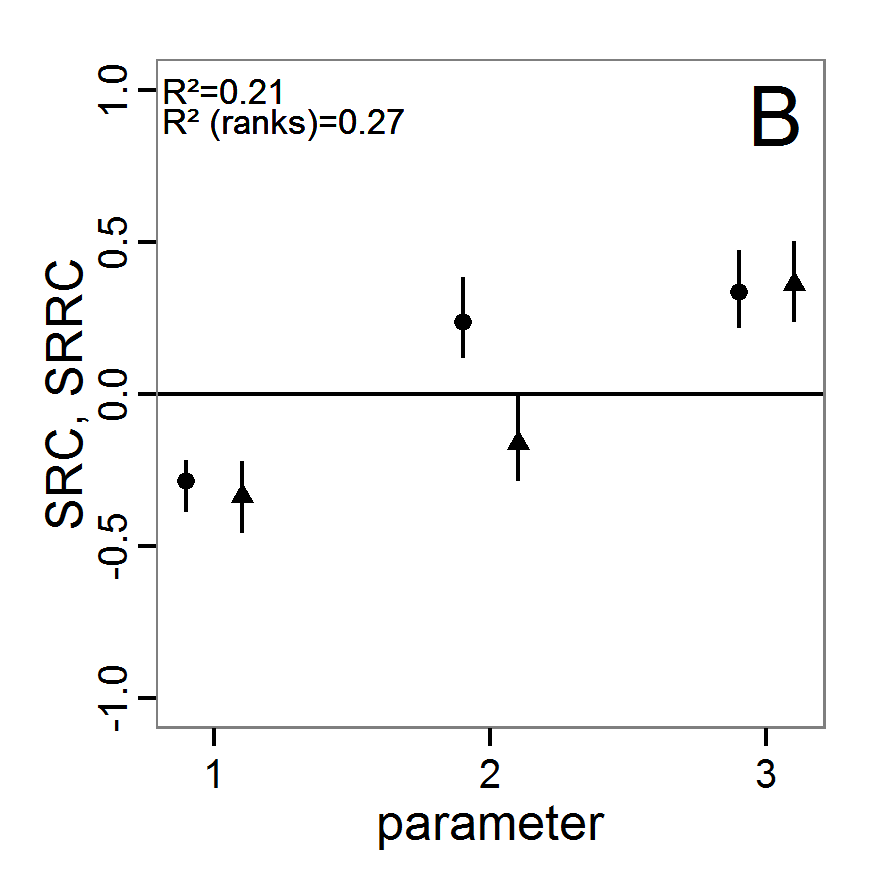

Figure 16. Results of the SRC/SRRC. A: for abundance output. B: for variation output. C: for vacancy output. Circles (to the left of each x-axis tick) show original SRC values (measure of linear relationship). Triangles (to the right of each x-axis tick) show original SRRC values (measure of linear or non-linear but monotonic relationship). Sticks show bootstrapped 95% confidence intervals of corresponding sensitivity indices. Numbers on x-axis for all plots: 1: scout-prob, 2: survival-prob, 3: scouting-survival. Top R2 in each plot corresponds to SRC and bottom R2 belongs to SRRC, giving the proportion of variation in the data captured by the regression model. - 3.35
- The results of an application of the SRC/SRRC method to the example model based on Latin hypercube sampling with 200 samples drawn from a uniform distribution for all parameters are given in Figure 16. Campolongo, Saltelli, et al. (2000) recommend calculating the coefficient of determination (R2), which is not processed by the sensitivity package. Therefore, we wrote a small function to calculate it (see Supplementary Material) because it tells us how well the linear regression model reproduces the output, i.e., how much of the output's variance is explained by the regression model (Campolongo, Saltelli, et al. 2000). In the case of non-linear relationships, using rank transformation (SRRC) can improve the R2 but will also alter the model because it becomes more additive and therefore includes less of the interaction effects (Campolongo, Saltelli, et al. 2000). In general, when there are strong interaction effects or non-monotonic relationships, R2 will be low and the application of SRC/SRRC is not very useful. Saltelli et al. (2008) recommend the usage of these methods only for models where R2 is greater than or equal to 0.7. As shown in Figure 16, this condition is met for the abundance and vacancy outputs but not for the variation output (panel B). Therefore, we should discard the results for the variation output. For the remaining two outputs, there is a strong dominance of the survival-prob input factor. There is only a small change in the coefficient values when using SRRC instead of SRC, and the R2s for SRC are already very high. This leads to the conclusion that there is a strong linear effect of survival-prob on these two outputs, with a positive sign for the abundance (SRC: 0.9865) and a negative sign for the vacancy output (SRC: –0.9987). Note that the absolute value of the SRC or SRRC gives a measure of the effect strength, and the sign defines the direction of the effect. All in all, the results are very similar to the findings with PCC/PRCC.
Variance decomposition methods
- 3.36
- For the investigation of non-linear and non-monotonic relationships between the inputs and outputs one should apply variance decomposition methods (Marino et al. 2008), but they can also be applied to models with monotonic and/or linear relationships. The three methods presented here are so-called total sensitivity indices (TSi) because they quantify the parameters' main effects as well as all interaction effects of any order (Ascough Il et al. 2005). These methods are, compared to the other sensitivity methods presented so far, computationally expensive. Therefore, it is recommended to first identify the important parameters by using, for example, Morris screening, and then restrict the variance decomposition methods to the most important parameters (Campolongo, Saltelli, et al. 2000).
- 3.37
- In analogy to ANOVA, the methods use techniques for the decomposition of the total variance of model output into first- (main) and higher-order (interaction) effects for each input factor (Confalonieri et al. 2010). When model input is varied, model output varies too, and the effect is measured by the calculation of statistical variance. Then, the part of the variance that can be explained by the variation of the input is determined (Marino et al. 2008).
Sobol' method
- 3.38
- The Sobol' method delivers a quantitative measure of the main and higher-order effects. It is very similar to effect calculation in DoE theory (Saltelli et al. 1999) and can be considered the adaptation of classical DoE to computer simulations. The idea is that the total variance is composed of the variance of the main and the interaction effects. Therefore, multiple integrals for the partial effect terms of different orders are extracted by decomposition and evaluated using Monte-Carlo methods instead of using factor levels, as is performed in classical DoE. For further details see, for example, the original work of Sobol' (1990) or that of Chan et al. (2000).
- 3.39
- An implementation of the Sobol' method can be found in the sensitivity package for R (Pujol et al. 2012). The sobol function is used in this way:
# 1. Define a simulation function (sim) as done for
# Full factorial design.
# 2. Create two random input factor samples (input.set.1,
# input.set.2) as required by the Sobol' method, for
# example two Latin hypercube samples
# (see also Partial (rank) correlation coefficient).
# 3. Create an instance of the class sobol using the result of step 2.
# Choose the order of variance decomposition:
so <- sobol(model = NULL, X1 = input.set.1,
X2 = input.set.2, order = 2, nboot = 100)
# 4. Get the simulated model response for all input factor
# combinations needed by the sobol method by calling the
# function defined in step 1.
sim.results <- apply(so$x, 1, sim)
# 5. Add the simulation results to the sobol instance.
tell(so, sim.results) - 3.40
- A modification of the Sobol' method exists that reduces the required number of model evaluations and delivers a main and total effect index, similar to the eFAST method. The implementation of this optimised method is also included in the sensitivity package (Pujol et al. 2012). The call of the sobol2007 function is similar to the sobol function with the exception that the number of orders of effects that should be calculated cannot be defined because this method cannot deliver single two- or higher-order effects explicitly as the original method can. Note that there are further modified versions of Sobol' algorithms available in the package sensitivity (see functions sobol2002, sobolEff and soboljansen).
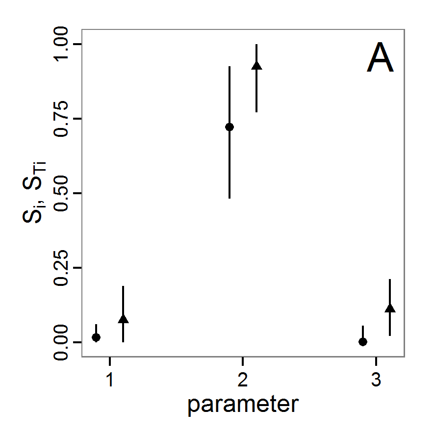
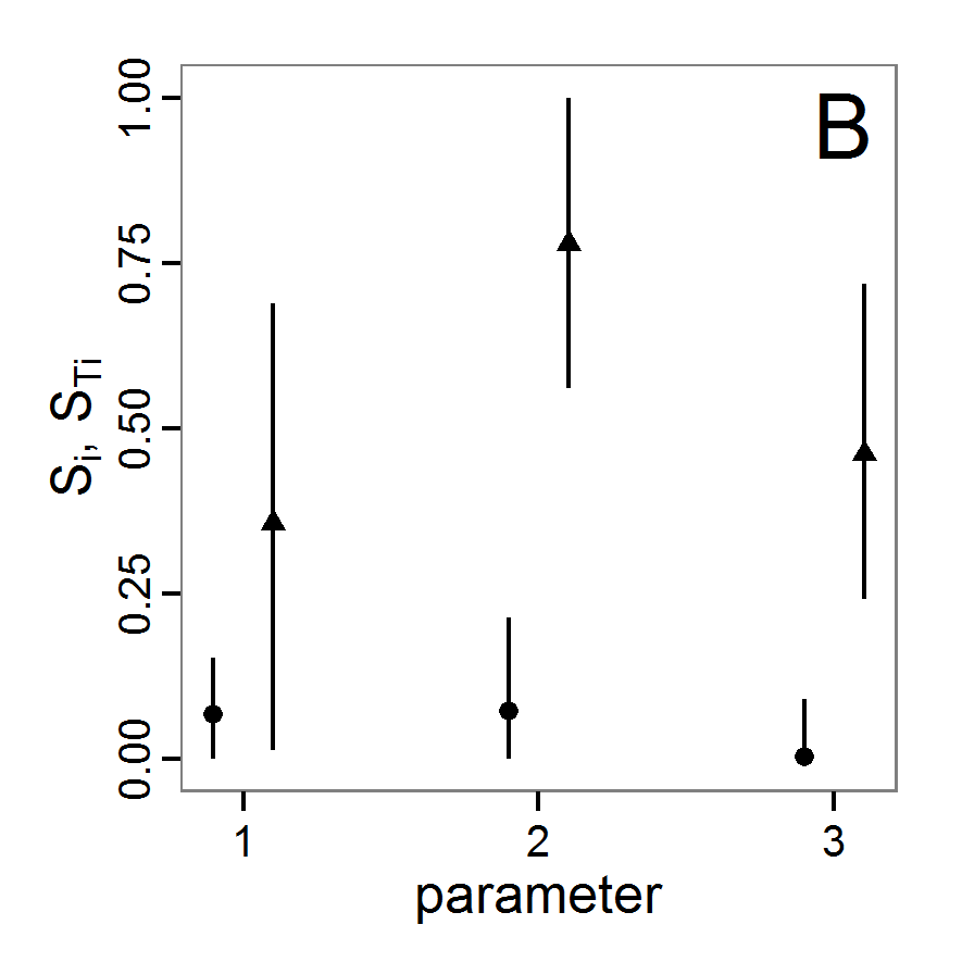
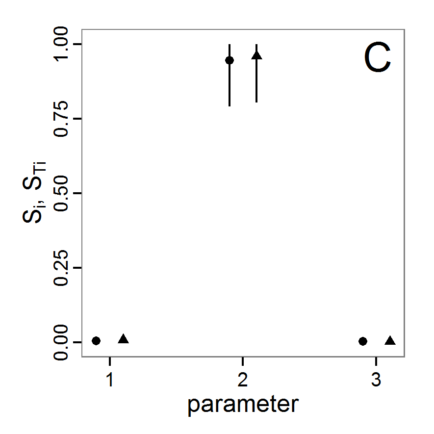
Figure 17. Results of the Sobol' method with modifications by Saltelli (sobol2007 function). A: for abundance output. B: for variation output. C: for vacancy output. Circles (to the left of each x-axis tick) show bias-corrected original first-order sensitivity index values (Si), i.e., main effects. Triangles (to the right of each x-axis tick) show bias-corrected original total sensitivity index values (STi), i.e., main and all interaction effects. Sticks show bootstrapped 95% confidence intervals of corresponding sensitivity indices. Negative values and values above 1, due to numerical errors, are set to 0 and 1, respectively. Numbers on x-axis for all plots: 1: scout-prob, 2: survival-prob, 3: scouting-survival. - 3.41
- The results of a usage example of the sobol2007 function with 3000 simulation function calls are shown in Figure 17. For every output and every input factor there are two candle sticks, the left one for the 95% confidence interval of the main/first-order effect index and the right one for the 95% confidence interval of the total effect index. When the confidence bands are very large, this can be an indicator of too-small samples. Furthermore, it can happen that the index values are negative or exceed 1 due to numerical errors in the calculation, but these can be treated as 0 and 1, respectively (Saltelli et al. 2008). The values of the indices are percentage measures of the contribution of the input factor to the variance of the output.
- 3.42
- For pure additive models, the sum of the main effect indices (Si) is 1; for others, it is below 1 and can never exceed 1 (only due to numerical errors). For example, the abundance output (panel A in Figure 17) sums up to approx. 0.74 (bias corrected), which means that the model is largely additive, i.e., only rather small interactions between the parameters occur, with a very strong contribution of the main effect of survival-prob (responsible for approx. 72% of the variation of the output). However, the quantification of the main effect contains considerable uncertainty, as indicated by the confidence interval. For the vacancy output (panel C), the contribution of survival-prob to the variance of the output is approx. 95%, i.e., the output variation depends nearly completely on the main effect of survival-prob. For the variation output (panel B), the main effects contribute only a very small proportion to the variance of the output. They sum up to approx. 13%.
- 3.43
- The total sensitivity index (STi) contains the main effect and all interaction effects with the other input factors. Therefore, it is often greater than the main effect index (Si). Equality between Si and STi means that the input factor has no interaction terms with the other input factors. In contrast to Si, the sum of all indices of STi is often greater than 1. Only if the model is perfectly additive, i.e., no interactions between the parameters exist, the sum is equal to 1 (Saltelli et al. 2008).
- 3.44
- In Figure 17, we see that there is nearly no interaction effect for the vacancy output (panel C), and the model is strongly additive. In contrast, strong interaction effects are uncovered by the STi for the variation output (panel B). The most important factor is survival-prob, but the confidence bands for all factors are large for STi, i.e., the conclusions are very uncertain. For the abundance output (panel A), we see an interaction effect explaining approx. 20% of the variance of the output and small interaction effects for the other two factors. Ostromsky et al. (2010) provide some rules of thumb for the categorisation of input factors. They classified input factors with total sensitivity index (STi) values of greater than 0.8 as very important, those with values between 0.5 and 0.8 as important, those with values between 0.3 and 0.5 as unimportant and those with values less than 0.3 as irrelevant. Using this classification, we come to the conclusion that the input factors scout-prob and scouting-survival are irrelevant for the abundance output, whereas survival-prob is very important. For the variation output, the input factor survival-prob is important whereas scout-prob and scouting-survival are unimportant (with high uncertainty), and for the vacancy output survival-prob is very important whereas the other two input factors are irrelevant.
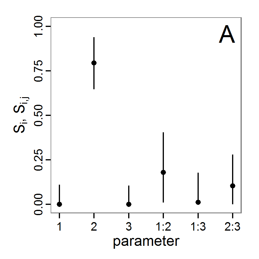
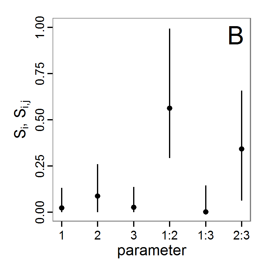
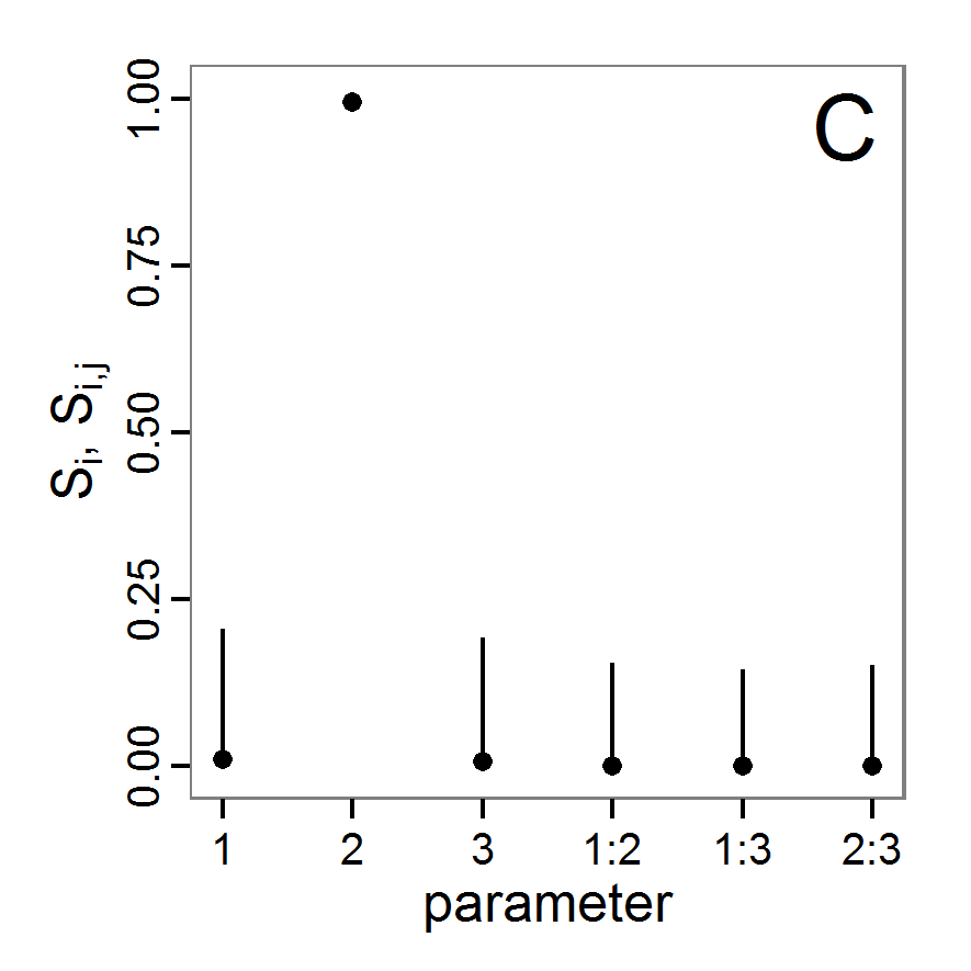
Figure 18. Results of the Sobol' method. A: for abundance output. B: for variation output. C: for vacancy output. Circles show bias-corrected original sensitivity index values. Sticks show bootstrapped 95% confidence intervals of corresponding sensitivity indices. Negative values and values above 1, due to numerical errors, are set to 0 and 1, respectively. Numbers on x-axis for all plots: 1: scout-prob, 2: survival-prob, 3: scouting-survival. Single numbers are main/first-order effects (Si) whereas numbers combined with colons show second-order interaction effects (Sij). - 3.45
- Applying the standard Sobol' method also enables us to analyse the higher-order effects separately. We calculated the Sobol' index up to the second order with 3500 simulation function calls (Figure 18). The results for the main effects exhibit the same pattern as described for the sobol2007 function but are numerically not exactly identical because this calculation is based on a new data sample. Taking into account second-order effects (Sij) shows that the main part of the interaction effects previously identified for survival-prob on the abundance output (panel A) results from interactions with both of the other input factors, scout-prob and scouting-survival, whereas there is no interaction effect between scout-prob and scouting-survival. For the variation output (panel B) we find the same pattern but with a much higher proportion of the interaction between scout-prob and survival-prob. This explains the very large differences between the main effect index and the total sensitivity index from function sobol2007 for the variation output (panel B). In accordance with the results of the sobol2007 function, we see no remarkable second-order sensitivity index value for the vacancy output in panel C.
- 3.46
- As we have seen, the Sobol' method is able to deliver all information needed for a comprehensive global sensitivity analysis. The method, however, is computationally more demanding than the other methods presented so far, and understanding the method in detail can be challenging.
Extended Fourier amplitude sensitivity test
- 3.47
- Extended Fourier amplitude sensitivity test (eFAST) uses, as the name suggests, Fourier series expansion to measure the strength of the influence of uncertain inputs on the model output. Being an extension of the original FAST (Cukier et al. 1973), eFAST adds the calculation of a total effects index (STi), which is the sum of main and all higher-order effects (Saltelli et al. 1999). For details on this method see Saltelli et al. (1999) or Chan et al. (2000). eFAST delivers the same measures of sensitivity as the Sobol' method (except specific interaction indices) but requires fewer simulations and is therefore computationally less expensive than the classical Sobol' method (Ravalico et al. 2005). Furthermore, it is more robust, especially at low sample sizes, to the choice of sampling points (Saltelli et al. 1999).
- 3.48
- The classical FAST algorithm is available in package fast for R (Reusser 2012), and the eFAST algorithm is included in the package sensitivity (Pujol et al. 2012). Using the fast99 function of the sensitivity package in R works in this way:
# 1. Define a simulation function (sim) as done for
# Full factorial design.
# 2. Create an instance of class fast99 with quantile
# functions for all input factors.
f99 <- fast99(model = NULL, factors = 3, n = 1000,
q = c("qunif","qunif","qunif"),
q.arg = list(list(min=0.0,max=0.5),
list(min=0.95,max=1.0),
list(min=0.5,max=1.0)))
# 3. Get the simulated model response for all input factor
# combinations needed by the fast99 method by calling the
# function defined in step 1.
sim.results <- apply(f99$x, 1, sim)
# 4. Add the simulation results to the fast99 instance.
tell(f99, sim.results) - 3.49
- The interpretation of the results of the eFAST method is the same as for the Sobol' method (function sobol2007). The method returns a main/first-order sensitivity index (Si) as well as a total sensitivity index (STi) that also contains interaction effects. Figure 19 shows the results based on 600 simulation function calls. The results are very similar to the results of the Sobol' method. There is a strong effect of input factor survival-prob for the abundance (panel A) and vacancy (panel C) outputs. There are nearly no interaction effects for the vacancy output and just minor interaction effects for the abundance output, whereas the main reasons for variance in the variation output are interaction effects. In contrast to the results of the Sobol' method from the previous section, here the input factor scout-prob explains slightly more of the variance in the variation output than the survival-prob input factor, whereas with the Sobol' method it was the other way around and the STi of scouting-survival was larger than the STi of scout-prob. The reasons for this could be due to differences in the methods themselves or to differences in the sampling schemes, too-small sample sizes, and/or a lack of convergence regarding stochastic effects, i.e., not enough replications for one parameter set. We have already observed that the confidence bands calculated for the Sobol' indices have been large, i.e., the results are uncertain. Therefore, it is not surprising that the results for the variation output differ. Nevertheless, the overall picture is the same between the Sobol' and eFAST methods. The choice of one or the other method depends primarily on the question of whether someone is interested only in main- and total-effect indices (then select eFAST; if confidence intervals are of interest then select the optimised Sobol' method), or if one wants also to know the second- and higher-order effect indices explicitly (then select the original Sobol' method, but keep in mind that it will not deliver total-effect indices).
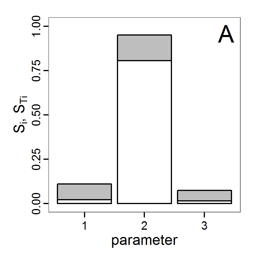
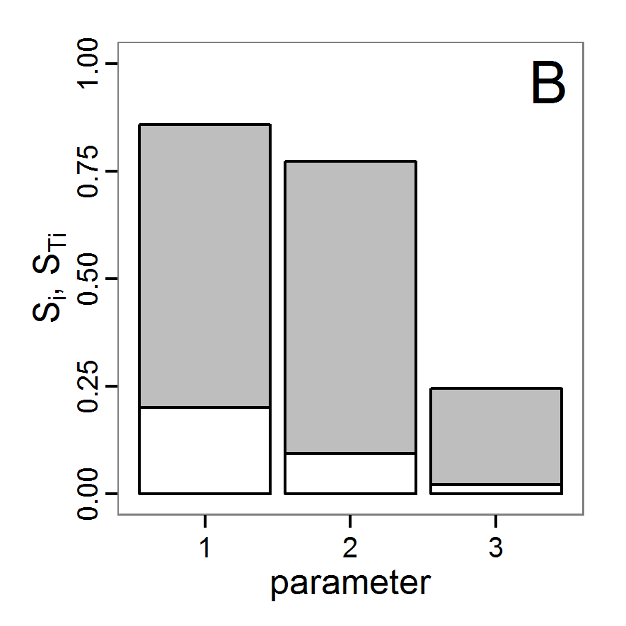
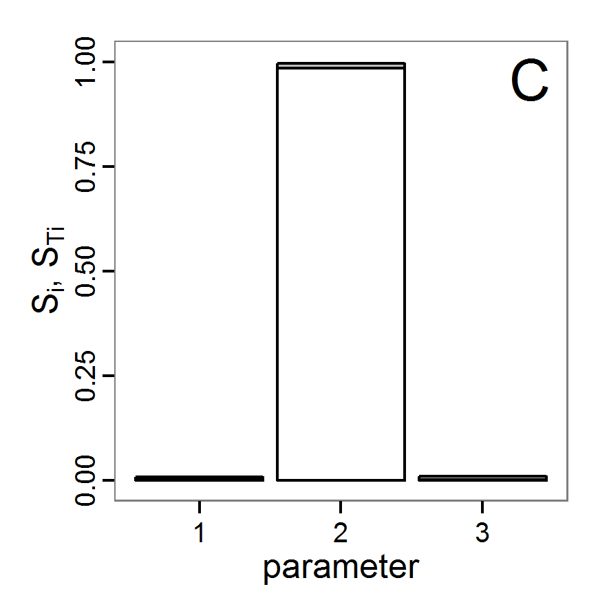
Figure 19. Results of the eFAST method. A: for abundance output. B: for variation output. C: for vacancy output. Numbers on x-axis for all plots: 1: scout-prob, 2: survival-prob, 3: scouting-survival. White bar: first-order effects (Si), i.e., main effects. Sum of white and grey bars: total effect (STi), i.e., main and all interaction effects. FANOVA decomposition with Gaussian process
- 3.50
- The method of fitting a Gaussian process (GP) to replace a computationally expensive model is related to the metamodel approach in DoE. A GP is a stochastic process, i.e., a generalisation of a probability distribution to functions of random variables, where each finite collection follows a joint (multivariate) normal distribution (Grimmett & Stirzaker 1993; Rasmussen & Williams 2006; Snelson 2007). GPs are used for interpolation, extrapolation and smoothing of time series (Wiener 1950) and spatial data. The geostatistical Kriging method, for example, is based on GPs (Snelson 2007). A GP, as a surrogate or emulator of a computer model, can be further used for a Functional Analysis of Variance (FANOVA), as performed by Dancik et al. (2010). The R package mlegpFULL (Dancik 2009, available on request from the developer of the online available mlegp package) can perform the fitting procedure and the FANOVA decomposition. The following shows how this works:
# 1. Run a Latin hypercube sampling as done above
# (see Partial (rank) correlation coefficient).
# The result should be two variables: the first containing
# the input factor combinations (param.sets) and the second
# containing the corresponding model responses (sim.results).
# 2. Fit a Gaussian process to the simulation results.
fit <- mlegp(param.sets, sim.results, param.names =
c('scout-prob',
'survival-prob',
'scout-survival'))
# 3. Calculate the FANOVA decomposition.
FANOVADecomposition(fit, verbose=FALSE) - 3.51
- We used a Latin hypercube sampling with only 500 samples, i.e., only 500 simulation function calls, to fit the Gaussian process. The results of the FANOVA decomposition using this Gaussian process are shown in Table 10. They contain results for main/first-order as well as second-order interaction effects but do not deliver total sensitivity indices as eFAST and Sobol' with modification by Saltelli do. Nevertheless, the results here are in good accordance with the results of the eFAST and Sobol' methods. The variation in the abundance output is mostly determined by the variation of the input factor survival-prob (ca. 81%), and there are only small second-order interaction effects. The second-order interaction effects here are primarily determined under participation of survival-prob with the other two input factors. There is nearly no interaction effect between scout-prob and scouting-survival, as we already know from the Sobol' method. The variance in variation output is determined to a large extent by the interaction effects of survival-prob with the other two input factors. The main effects are less important, but the ranking of importance of the three input factors differs in comparison to the eFAST and Sobol' methods. From the Sobol' method we already know that the results for the variation output are uncertain. Therefore, this difference is not surprising. For the vacancy output the results here again fully match the results of the eFAST and Sobol' methods. The most important factor is survival-prob, explaining approx. 99% of the variance with its first-order effect (eFast: 98%, Sobol': 99%, optimised Sobol': 95%).
Table 10: Results of the FANOVA decomposition method using a fitted Gaussian process. Names in the first column are the input factors. Single names are main effects. Names combined with a colon are (second-order) interaction effects. abundance variation vacancy scout-prob 1.733 10.984 0.107 survival-prob 80.561 13.272 98.828 scouting-survival 2.487 12.160 0.022 scout-prob:survival-prob 5.820 31.400 0.653 scout-prob:scouting-survival 0.134 2.862 0.022 survival-prob:scouting-survival 4.655 26.914 0.530 - 3.52
- Overall, the results fit very well with the results of the other variance decomposition methods even though we used fewer simulation runs. Nevertheless, FANOVA decomposition can only be as good as the Gaussian process is, and the goodness of fit is limited by how well the sample represents the simulation model behaviour with respect to the varied input factors, which depends primarily on the sampling design and the number of samples. Furthermore, the GP is only useful in cases where the response surface is a smooth function of the parameter space (Dancik et al. 2010).
Costs and benefits of approaches to sensitivity analysis
- 3.53
- In the previous section we presented different sensitivity analysis techniques. Despite the fact that it is impossible to list all existing methods, we presented, from our point of view, the most commonly used and interesting ones in the context of ABMs and provided starting points for adaptations to others. In Figure 20, we compare the methods presented here in the same manner as the fitting methods in the intermediate discussion (see Figure 11). There is quite some overlap between the different methods, and the ranking in terms of costs and gains is not as clear as with the fitting methods. Furthermore, the purposes of the methods as well as their requirements for the models are different.
- 3.54
- As with the fitting methods, for sensitivity analysis it is often useful to start with a simple method and then apply a more informative but computationally more demanding method to explore only the most important input factors. It is always a good idea to start with a graphical method, e.g., scatterplots, to obtain a rough feeling for the relationships of inputs and outputs and their linearity or non-linearity. In a next step, one can, for example, use Morris's elementary effects screening to identify the most important factors and apply the Sobol' method afterwards to these factors or, as performed by Marino et al. (2008), apply the partial (rank) correlation coefficient method first and use the eFAST method afterwards.
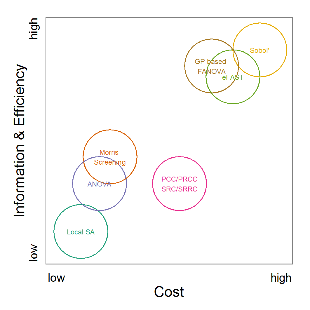
Figure 20. Rough categorisation of sensitivity methods used regarding their cost vs. information and efficiency. Cost includes the computational costs (i.e., number of simulations, which depend itself on the model and the number of parameters) as well as the time consumed by fine-tuning of the methods. Information and efficiency includes aspects about the type of output and the way reaching it. Partly adapted from Campolongo et al. (1999).
Discussion
- 4.1
- One might argue that most ABMs are too complex and computationally expensive to run them hundreds or thousands of times with varying parameter values and starting conditions for parameter fitting or sensitivity analysis. However, the way for ABM to become an accepted research method is not to make the models as realistic and complex as possible. An important, if not decisive, design criterion for ABMs, as well as any other simulation models, is that they must run quickly enough to be amenable to comprehensive and systematic analysis. This requires that a single run should be fast enough to allow for both interactive cursory and automatic systematic model analysis. Thus, it is essential to test submodels and make a great effort to find the simplest ones that still serve their purpose.
- 4.2
- There can be limits to simplification, for example if a model is no longer able to reproduce multiple patterns simultaneously (Grimm & Railsback 2012; Railsback & Grimm 2012); in such cases, using computing clusters, which currently are often available, can help to still perform the high number of simulations required by some of the methods described here.
- 4.3
- A point we have so far not discussed in detail is the variability of simulation outputs caused by stochastic components, which are usually included in ABMs. A single simulation run may thus not be representative for the spectrum of possible simulation outputs. Using different seeds for the function generating random numbers can result in completely different dynamics.
- 4.4
- This issue is often addressed in textbooks about agent-based modelling (e.g., North & Macal 2007; Railsback & Grimm 2012; Squazzoni 2012; Tesfatsion & Judd 2006). It is recommended to run a model with the same configuration repeatedly with different random seeds. Then, the mean of the model outputs is calculated, as we did here; confidence intervals should also be calculated. However, this solution implies two further issues. First, the question of how many iterations are needed must be answered. The classical textbooks do not answer this question. It is often solved by an ad hoc definition that, for example,10 or 50 replications are sufficient for a specific model (e.g., Kerr et al. 2002; Martínez et al. 2011; Arifin et al. 2013; Railsback & Grimm 2012; Squazzoni 2012). Very likely, just 10 iterations, as used here, will often not be enough. However, an established general accepted strategy for finding an adequate number of repetitions is missing. Nikolic et al. (2013) recommend performing a LHS over the parameter space with 100 replicated runs for each parameter set to identify the most variable metric and parameter value set. Then, this parameter value set producing the most variable metric is used to estimate the number of replications needed to gain a defined confidence level. A similar approach was applied by Kelso and Milne (2011). In combination with the method suggested by Lorscheid et al. (2012), discussed at the beginning of this article, it is a good starting point to avoid ad hoc assumptions about appropriate replication numbers while a general strategy is missing. This approach becomes less reliable when non-linear processes are involved but is the best approach currently available in terms of the cost-benefit ratio.
- 4.5
- The second issue affects the interpretation of the output of ABMs: variation in model output represents variation in reality, i.e., in environmental drivers and the properties and behaviours of a model's entities. Ignoring this variation by only considering averaged model outputs might thus be misleading. Still, averages should capture overall trends, and sensitivity analyses should thus still be informative of the relative importance of processes. The sensitivity of model output to uncertainties in model inputs, though, might be blurred by the stochasticity inherent to the system to be represented. Real uncertainty might thus be higher than the uncertainty detected by sensitivity analyses, which is focused on averaged model outputs. Therefore, it might often be advisable to consider not only the sensitivity of the averaged outputs but also that of the variance of the outputs.
- 4.6
- Sensitivity analyses can help understand how a model works, but it should be noted that at least two more general approaches will usually be required for full understanding: simulation experiments and some type of regression analysis. In simulation experiments, one parameter at a time is varied over its full range, and the response of one or more output metrics is studied. These experiments are usually designed like real experiments: only one or a few factors are varied systematically, whereas all other factors are kept constant. Simulation experiments are basically designed to test simple hypotheses, i.e., the model settings are "controlled" to such a degree that we can make predictions of how the model should behave. Important typical experiments include the use of extreme parameter values; turning processes on and off; exploring smaller systems; exploring submodels separately; making drivers constant; making the environment spatially more homogeneous, etc.
- 4.7
- With regression analysis, we here refer to statistical methods that explore how much certain processes, represented by their corresponding parameters, affect one or more model outputs. Typical approaches for this include analysis of variance, generalised linear models, regression trees, path analysis, and many more. For all of these methods, packages exist in R, so they can in principle be used for analysing ABMs in the same way as done here for sensitivity analysis.
- 4.8
- Some readers, if not the majority, might have been lost while reading about the more complex methods described here, primarily because they are not familiar with the statistical methods employed for interpreting the results of the sensitivity analyses. Still, we always tried to describe in detail what the output of the analyses means in terms of the sensitivity of single parameters, or parameter interactions, and all this for different model outputs. After such detailed and partly technical considerations, it is always important to step back and ask yourself the following: what have we learned about the relative importance of processes, how processes interact, and how uncertainties in parameter values would affect simulation results?
- 4.9
- For our example model, the main lessons learned are as follows: All three tested parameters have a considerable influence on the model results, or, expressed the other way round, the model is sensitive to variations in these parameter values. However, the influence strongly differs regarding both the output measure considered and the parameters. Therefore, it is important to not analyse simulation results on the basis of a single output measure.
- 4.10
- In all analyses, survival-prob has been identified as the most important parameter. This is not surprising, as this survival probability affects all individuals every month. We varied this probability by only 5 per cent. This means, on the one hand, that the population is very vulnerable regarding its survival probability, and on the other hand, that the more uncertain the value of survival-prob is, the more uncertain the models' outputs are, for example, assessments of extinction risks. Is this sensitivity real, or is it an artefact of the selected model structure? In reality, individuals are different, so some individuals should have a higher survival chance than others. It has been shown that this variability serves as a "buffer mechanism", reducing extinction risk (Grimm, Revilla, Groeneveld et al. 2005).
- 4.11
- Still, even if we focus on survival probability as represented in the example model, improving survival to reduce extinction risk might not be sufficient because there are considerable interaction effects, especially regarding the standard deviation of the annual abundance (variation criterion). Although the main-effects of scout-prob and scouting-survival were unimportant, their influence caused by interactions with survival-prob was very important for the variation criterion. Furthermore, we observed both linear effects and non-linear effects of parameter variations.
- 4.12
- We based the technical implementation on two commonly used software tools, NetLogo and R. R in particular, with its many user-contributed packages, delivers all commonly used methods for parameter fitting and sensitivity analysis. Nevertheless, we would again like to remind readers of other tools for parameter fitting and/or sensitivity analysis for models implemented in NetLogo. The most prominent ones are BehaviorSearch (Stonedahl & Wilensky 2013), openMole (Reuillon et al. 2010), MASS/MEME (Iványi et al. 2007), and Simlab (Simlab 2012). Other general-purpose statistical/mathematical software systems, such as MatLab (The MathWorks Inc. 2010) and Mathematica (Wolfram Research 2010), also provide many of the described methods, but these systems are mostly proprietary.
- 4.13
- What we wanted to foster with this "cookbook" is to avoid re-inventing the wheel. In young research areas, such as the field of agent-based modelling, it is common for users to implement their own solutions when standards are missing. Often, however, several components have already been implemented. We believe that re-inventing the wheel in every ABM project is a major waste of time and money and liable to introduce errors. Rather than trying to implement existing methods from scratch, or trying something new but untested, one should try and use existing tested software tools. This is in contrast to the everyday practice of most agent-based modellers, who are accustomed to programming virtually everything from scratch. With regard to parameterisation and sensitivity analysis, this ad hoc approach would be inefficient and highly uncertain.
- 4.14
- We hope that our cookbook lowers the threshold for using fitting and sensitivity analysis methods in ABM studies and delivers a contribution towards rigorous agent-based modelling. Nevertheless, this paper cannot (and is not intended to) replace the intensive study of more detailed literature about these topics and the specific methods. It was our intention to give a rough overview of the most popular methods available to make modellers aware of them. Furthermore, we wanted to show what the methods can bring to modellers and how to apply the methods to an agent-based model in a reusable way. We based the technical implementation on two commonly used software tools, NetLogo and R, to achieve a less steep learning curve. Moreover, both NetLogo and R are supported by large user groups and have established discussion forums on the internet, where beginners can post questions regarding the methods presented here or browse the forums' archives for similar questions.
- 4.15
- Still, reading a cookbook does not make you a chef; it only shows you how to start and gives you an idea of what you could achieve if you work hard enough. We hope that this contribution helps more ABM cooks to produce wonderful meals: models that aid in understanding, in a predictive way, and managing real agent-based complex systems.
Acknowledgements
- We thank Klaus G. Troitzsch, Nigel Gilbert, Gary Polhill and Cyril Piou for their helpful comments on earlier drafts. Furthermore, we thank Gilles Pujol for his work on the sensitivity package and Garrett Dancik for his work on the mlegp/mlegpFULL package.
References
-
AARTS, E., & Korst, J. (1989). Simulated Annealing and Boltzmann Machines. Chichester: Wiley.
ARIFIN, S., Madey, G., & Collins, F. (2013). Examining the Impact of Larval Source Management and Insecticide-Treated Nets Using a Spatial Agent-Based Model of Anopheles Gambiae and a Landscape Generator Tool. Malaria Journal, 12(1), 290. [doi:10.1186/1475-2875-12-290]
ASCOUGH IL, J., Green, T., Ma, L., & Ahjua, L. (2005). Key Criteria and Selection of Sensitivity Analysis Methods Applied to Natural Resource Models (pp. 2463–2469). Presented at the Modsim 2005 International Congress on Modeling and Simulation, Modeling and Simulation Society of Australia and New Zealand, Melbourne. http://www.mssanz.org.au/modsim05/papers/ascough_2.pdf Archived at: http://www.webcitation.org/6MlOGzavB
BACK, T. (1996). Evolutionary Algorithms in Theory and Practice: Evolution Strategies, Evolutionary Programming, Genetic Algorithms. Oxford: Oxford University Press.
BAKSHY, E., & Wilensky, U. (2007). Turtle Histories and Alternate Universes; Exploratory Modeling with NetLogo and Mathematica. In M. North, C. Macal, & D. Sallach (Eds.), Proceedings of the Agent 2007 Conference on Complex Interaction and Social Emergence (pp. 147–158). L'Argonne National Laboratory and Northwestern University.
BANSAL, R. (2005). Optimization Methods for Electric Power Systems: An Overview. International Journal of Emerging Electric Power Systems, 2(1). [doi:10.2202/1553-779X.1021]
BAR MASSADA, A., & Carmel, Y. (2008). Incorporating Output Variance in Local Sensitivity Analysis for Stochastic Models. Ecological Modelling, 213(3-4), 463–467. [doi:10.1016/j.ecolmodel.2008.01.021]
BEAUMONT, M. (2010). Approximate Bayesian Computation in Evolution and Ecology. Annual Review of Ecology, Evolution, and Systematics, 41(1), 379–406. [doi:10.1146/annurev-ecolsys-102209-144621]
BEAUMONT, M., Zhang, W., & Balding, D. (2002). Approximate Bayesian Computation in Population Genetics. Genetics, 162(4), 2025–2035.
BIETHAHN, J., Lackner, A., & Range, M. (2004). Optimierung und Simulation. München: Oldenbourg.
BLOWER, S., & Dowlatabadi, H. (1994). Sensitivity and Uncertainty Analysis of Complex Models of Disease Transmission: An HIV Model, as an Example. International Statistical Review / Revue Internationale de Statistique, 62(2), 229–243. [doi:10.2307/1403510]
BONNANS, J.-F., Gilbert, J., Lemarechal, C., & Sagastizábal, C. (2006). Numerical Optimization: Theoretical and Practical Aspects (2nd ed.). Berlin/Heidelberg: Springer.
BOX, G. E. P., Hunter, W. G., & Hunter, J. S. (1978). Statistics for Experimenters: An Introduction to Design, Data Analysis, and Model Building. Wiley series in probability and mathematical statistics. New York: Wiley.
BYRD, R., Lu, P., Nocedal, J., & Zhu, C. (1995). A Limited Memory Algorithm for Bound Constrained Optimization. SIAM Journal on Scientific Computing, 16(5), 1190–1208. [doi:10.1137/0916069]
CALVEZ, B., & Hutzler, G. (2006). Automatic Tuning of Agent-Based Models Using Genetic Algorithms. In J. Sichman & L. Antunes (Eds.), Multi-Agent Based Simulation VI, Lecture Notes in Computer Science (pp. 41–57). Berlin/Heidelberg: Springer. [doi:10.1007/11734680_4]
CAMPOLONGO, F., Cariboni, J., & Saltelli, A. (2007). An Effective Screening Design for Sensitivity Analysis of Large Models. Environmental Modelling & Software, 22(10), 1509–1518. [doi:10.1016/j.envsoft.2006.10.004]
CAMPOLONGO, F., Kleijnen, J., & Andres, T. (2000). Screening Methods. In A. Saltelli, K. Chan, & E. Scott (Eds.), Sensitivity Analysis (pp. 65–80). Chichester: Wiley.
CAMPOLONGO, F., & Saltelli, A. (2000). Design of Experiments. In A. Saltelli, K. Chan, & E. Scott (Eds.), Sensitivity Analysis (pp. 51–63). Chichester: Wiley.
CAMPOLONGO, F., Saltelli, A., Sorensen, T., & Tarantola, S. (2000). Hitchhiker's Guide to Sensitivity Analysis. In A. Saltelli, K. Chan, & E. Scott (Eds.), Sensitivity Analysis (pp. 17–47). Chichester: Wiley.
CAMPOLONGO, F., Tarantola, S., & Saltelli, A. (1999). Tackling Quantitatively Large Dimensionality Problems. Computer Physics Communications, 117(1–2), 75–85. [doi:10.1016/S0010-4655(98)00165-9]
CARIBONI, J., Gatelli, D., Liska, R., & Saltelli, A. (2007). The Role of Sensitivity Analysis in Ecological Modelling. Ecological Modelling, 203(1–2), 167–182. [doi:10.1016/j.ecolmodel.2005.10.045]
CARNELL, R. (2012). lhs: Latin Hypercube Samples. http://cran.r-project.org/web/packages/lhs/ Archived at: http://www.webcitation.org/6H9MePfSw
CERDEIRA, J., Silva, P., Cadima, J., & Minhoto, M. (2012). subselect: Selecting Variable Subsets. http://cran.r-project.org/web/packages/subselect Archived at: http://www.webcitation.org/6H9MsDvZK
CHAN, K., Tarantola, S., Saltelli, A., & Sobol', I. (2000). Variance-Based Methods. In A. Saltelli, K. Chan, & E. Scott (Eds.), Sensitivity Analysis (pp. 167–197). Chichester: Wiley.
CONFALONIERI, R., Bellocchi, G., Bregaglio, S., Donatelli, M., & Acutis, M. (2010). Comparison of Sensitivity Analysis Techniques: A Case Study With the Rice Model WARM. Ecological Modelling, 221(16), 1897–1906. [doi:10.1016/j.ecolmodel.2010.04.021]
COURNÈDE, P.-H., Chen, Y., Wu, Q., Baey, C., & Bayol, B. (2013). Development and Evaluation of Plant Growth Models: Methodology and Implementation in the PYGMALION platform. Mathematical Modelling of Natural Phenomena, 8(4), 112–130. [doi:10.1051/mmnp/20138407]
CRAWLEY, M. (2005). Statistics: An Introduction Using R. Chichester: Wiley. [doi:10.1002/9781119941750]
CSILLERY, K., Blum, M., & Francois, O. (2012). abc: Tools for Approximate Bayesian Computation (ABC). http://cran.r-project.org/web/packages/abc Archived at: http://www.webcitation.org/6H9Mx9bQ1
CSILLERY, K., Francois, O., & Blum, M. (2012). Approximate Bayesian Computation (ABC) in R: A Vignette. http://cran.r-project.org/web/packages/abc/vignettes/abcvignette.pdf Archived at: http://www.webcitation.org/6H9N0oSlv
CUKIER, R., Fortuin, C., Shuler, K., Petschek, A., & Schaibly, J. (1973). Study of the Sensitivity of Coupled Reaction Systems to Uncertainties in Rate Coefficients. I Theory. The Journal of Chemical Physics, 59, 3873–3878. [doi:10.1063/1.1680571]
DALGAARD, P. (2008). Introductory Statistics with R (2nd ed.). New York: Springer. [doi:10.1007/978-0-387-79054-1]
DANCIK, G. (2009). mlegpFULL: Maximum Likelihood Estimates of Gaussian Processes. (available from author on request, see http://cran.r-project.org/web/packages/mlegp/index.html Archived at: http://www.webcitation.org/6MlT9MYsu)
DANCIK, G., Jones, D., & Dorman, K. (2010). Parameter Estimation and Sensitivity Analysis in an Agent-Based Model of Leishmania Major Infection. Journal of Theoretical Biology, 262(3), 398–412. [doi:10.1016/j.jtbi.2009.10.007]
DUBOZ, R., Versmisse, D., Travers, M., Ramat, E., & Shin, Y.-J. (2010). Application of an Evolutionary Algorithm to the Inverse Parameter Estimation of an Individual-Based Model. Ecological Modelling, 221(5), 840–849. [doi:10.1016/j.ecolmodel.2009.11.023]
DUPUY, D., & Helbert, C. (2011). DiceEval: Construction and Evaluation of Metamodels. http://CRAN.R-project.org/package=DiceEval Archived at: http://www.webcitation.org/6MlOvl3GE
FIELDING, M. (2011). MCMChybridGP: Hybrid Markov Chain Monte Carlo Using Gaussian Processes. http://cran.r-project.org/web/packages/MCMChybridGP/ Archived at: http://www.webcitation.org/6H9N6EAbv
FLETCHER, R. (1987). Practical Methods of Optimization (2nd ed.). Chichester: Wiley.
FROST, C., Hygnstrom, S., Tyre, A., Eskridge, K., Baasch, D., Boner, J., Clements, G., et al. (2009). Probabilistic Movement Model with Emigration Simulates Movements of Deer in Nebraska, 1990–2006. Ecological Modelling, 220(19), 2481–2490. [doi:10.1016/j.ecolmodel.2009.06.028]
GAN, Y., Duan, Q., Gong, W., Tong, C., Sun, Y., Chu, W., Ye, A., et al. (2014). A Comprehensive Evaluation of Various Sensitivity Analysis Methods: A Case Study With a Hydrological Model. Environmental Modelling & Software, 51, 269–285. [doi:10.1016/j.envsoft.2013.09.031]
GEYER, C., & Johnson, L. (2013). mcmc: Markov Chain Monte Carlo. http://cran.r-project.org/web/packages/mcmc/ Archived at: http://www.webcitation.org/6H9NC0Gow
GILBERT, N. (2007). Agent-Based Models. Los Angeles: Sage.
GINOT, V., Gaba, S., Beaudouin, R., Aries, F., & Monod, H. (2006). Combined Use of Local and ANOVA-Based Global Sensitivity Analyses for the Investigation of a Stochastic Dynamic Model: Application to the Case Study of an Individual-Based Model of a Fish Population. Ecological Modelling, 193(3–4), 479–491. [doi:10.1016/j.ecolmodel.2005.08.025]
GRAMACY, R., & Taddy, M. (2013). tgp: Bayesian Treed Gaussian Process Models. http://cran.r-project.org/web/packages/tgp/ Archived at: http://www.webcitation.org/6H9NH3MZD
GRIMM, V. (2008). Individual-Based Models. In S. Jørgensen (Ed.), Ecological Models (pp. 1959–1968). Oxford: Elsevier. [doi:10.1016/b978-008045405-4.00188-9]
GRIMM, V., Berger, U., DeAngelis, D., Polhill, G., Giske, J., & Railsback, S. (2010). The ODD Protocol: A Review and First Update. Ecological Modelling, 221(23), 2760–2768. [doi:10.1016/j.ecolmodel.2010.08.019]
GRIMM, V., & Railsback, S. (2005). Individual-Based Modeling and Ecology. Princeton: Princeton University Press. [doi:10.1515/9781400850624]
GRIMM, V., & Railsback, S. (2012). Pattern-oriented Modelling: A "Multi-scope" for Predictive Systems Ecology. Philosophical Transactions of the Royal Society B: Biological Sciences, 367(1586), 298–310. [doi:10.1098/rstb.2011.0180]
GRIMM, V., Revilla, E., Berger, U., Jeltsch, F., Mooij, W., Railsback, S., Thulke, H.-H., et al. (2005). Pattern-Oriented Modeling of Agent-Based Complex Systems: Lessons from Ecology. Science, 310(5750), 987–991. [doi:10.1126/science.1116681]
GRIMM, V., Revilla, E., Groeneveld, J., Kramer-Schadt, S., Schwager, M., Tews, J., Wichmann, M., et al. (2005). Importance of Buffer Mechanisms for Population Viability Analysis. Conservation Biology, 19(2), 578–580. [doi:10.1111/j.1523-1739.2005.000163.x]
GRIMMETT, G., & Stirzaker, D. (1993). Probability and Random Processes (2nd ed., reprint.). Oxford: Clarendon Press.
GROEMPING, U. (2011). FrF2: Fractional Factorial Designs with 2-Level Factors. http://cran.r-project.org/web/packages/FrF2/ Archived at: http://www.webcitation.org/6H9NO65Hn
GROEMPING, U. (2013a). CRAN Task View: Design of Experiments (DoE) & Analysis of Experimental Data. http://cran.r-project.org/web/views/ExperimentalDesign.html Archived at: http://www.webcitation.org/6H9NRcCYN
GROEMPING, U. (2013b). DoE.base: Full Factorials, Orthogonal Arrays and Base Utilities for DoE Packages. http://cran.r-project.org/web/packages/DoE.base/ Archived at: http://www.webcitation.org/6H9NV5KCl
GUICHARD, S., Kriticos, D. J., Kean, J. M., & Worner, S. P. (2010). Modelling Pheromone Anemotaxis for Biosecurity Surveillance: Moth Movement Patterns Reveal a Downwind Component of Anemotaxis. Ecological Modelling, 221(23), 2801–2807. [doi:10.1016/j.ecolmodel.2010.08.030]
HAMBY, D. M. (1995). A Comparison of Sensitivity Analysis Techniques. Health Physics, 68(2), 195–204. [doi:10.1097/00004032-199502000-00005]
HAN, L., Da Silva, D., Boudon, F., Cokelaer, T., Pradal, C., Faivre, R., & Costes, E. (2012). Investigating the Influence of Geometrical Traits on Light Interception Efficiency of Apple Trees: A Modelling Study with MAppleT. In M. Kang, Y. Dumont, & Y. Guo (Eds.), Fourth International Symposium on Plant Growth Modeling, Simulation, Visualization and Applications (pp. 152–159). IEEE Press. http://hal.inria.fr/docs/00/79/06/50/PDF/Han_etal_PMA2012_26-2.pdf Archived at: http://www.webcitation.org/6MlPQm4tv [doi:10.1109/pma.2012.6524827]
HAPPE, K. (2005). Agent-Based Modelling and Sensitivity Analysis by Experimental Design and Metamodelling: An Application to Modelling Regional Structural Change. Presented at the European Association of Agricultural Economists 2005 International Congress, Copenhagen, Denmark. http://purl.umn.edu/24464 Archived at: http://www.webcitation.org/6MlPFiZqu
HARTIG, F., Calabrese, J., Reineking, B., Wiegand, T., & Huth, A. (2011). Statistical Inference for Stochastic Simulation Models – Theory and Application. Ecology Letters, 14(8), 816–827. [doi:10.1111/j.1461-0248.2011.01640.x]
HARTIG, F., Dislich, C., Wiegand, T., & Huth, A. (2013). Technical Note: Approximate Bayesian Parameterization of a Complex Tropical Forest Model. Biogeosciences Discuss., 10(8), 13097–13128. [doi:10.5194/bgd-10-13097-2013]
HASTIE, T. (2011). gam: Generalized Additive Models. http://CRAN.R-project.org/package=gam Archived at: http://www.webcitation.org/6MlPWODr8
HELTON, J., Hiermer, J., Sallaberry, C., & Storlie, C. (2006). Survey of Sampling-Based Methods for Uncertainty and Sensitivity Analysis. Reliability Engineering & System Safety, 91(10–11), 1175–1209. [doi:10.1016/j.ress.2005.11.017]
HOLLAND, J. (2001). Adaptation in Natural and Artificial Systems: An Introductory Analysis with Applications to Biology, Control and Artificial Intelligence (6th ed.). Cambridge: MIT Press.
HOTHORN, T. (2013). CRAN Task View: Machine Learning & Statistical Learning. http://cran.r-project.org/web/views/MachineLearning.html Archived at: http://www.webcitation.org/6H9NZJFa0
HYNDMAN, R. (2013). CRAN Task View: Time Series Analysis. http://cran.r-project.org/web/views/TimeSeries.html Archived at: http://www.webcitation.org/6H9NdY31r
IMRON, M., Gergs, A., & Berger, U. (2012). Structure and Sensitivity Analysis of Individual-Based Predator–Prey Models. Reliability Engineering & System Safety, 107, 71–81. [doi:10.1016/j.ress.2011.07.005]
IVÁNYI, M., Gulyás, L., Bocsi, R., Szemes, G., & Mészáros, R. (2007). Model Exploration Module (pp. 207–215). Presented at the Agent 2007, Evanston, IL. http://www.dis.anl.gov/pubs/60568.pdf Archived at: http://www.webcitation.org/6H9Nqgeqd
JABOT, F., Faure, T., & Dumoulin, N. (2013). EasyABC: Performing Efficient Approximate Bayesian Computation Sampling Schemes Using R. Methods in Ecology and Evolution. [doi:10.1111/2041-210X.12050]
JAKOBY, O., Grimm, V., & Frank, K. (2014). Pattern-oriented Parameterization of General Models for Ecological Application: Towards realistic Evaluations of Management Approaches. Ecological Modelling, 275, 78-88. [doi:10.1016/j.ecolmodel.2013.12.009]
KELSO, J., & Milne, G. (2011). Stochastic Indiviual-Based Modelling of Influenza Spread for the Assessment of Public Health Interventions. Presented at the 19th International Congress on Modelling and Simulation, Perth, Austrialia. http://www.mssanz.org.au/modsim2011/B2/kelso.pdf Archived at: http://www.webcitation.org/6MlPgqAad
KERR, B., Riley, M. A., Feldman, M. W., & Bohannan, B. J. M. (2002). Local Dispersal Promotes Biodiversity in a Real-Life Game of Rock-Paper-Scissors. Nature, 418(6894), 171–174. [doi:10.1038/nature00823]
KING, A., Ionides, E., Breto, C., Ellner, S., Ferrari, M., Kendall, B., Lavine, M., et al. (2013). pomp: Statistical inference for partially observed Markov processes (R package). http://cran.r-project.org/web/packages/pomp/index.html Archived at: http://www.webcitation.org/6KdUJrXfv
KLEIJNEN, J. (1995). Sensitivity Analysis and Related Analysis: A Survey of Statistical Techniques. October 6, 2011, http://econpapers.repec.org/paper/dgrkubrem/1995706.htm Archived at: http://www.webcitation.org/6MlPnSnDV
KLEIJNEN, J. (2008). Design and Analysis of Simulation Experiments. New York, NY: Springer.
LENTH, R. (2009). Response-Surface Methods in R, Using rsm. Journal of Statistical Software, 32(7), 1–17. [doi:10.18637/jss.v032.i07]
LORSCHEID, I., Heine, B.-O., & Meyer, M. (2012). Opening the "Black Box" of Simulations: Increased Transparency and Effective Communication Through the Systematic Design of Experiments. Computational and Mathematical Organization Theory, 18(1), 22–62. [doi:10.1007/s10588-011-9097-3]
LUNN, D., Spiegelhalter, D., Thomas, A., & Best, N. (2009). The BUGS Project: Evolution, Critique and Future Directions. Statistics in Medicine, 28(25), 3049–3067. [doi:10.1002/sim.3680]
MARINO, S., Hogue, I., Ray, C., & Kirschner, D. (2008). A Methodology for Performing Global Uncertainty and Sensitivity Analysis in Systems Biology. Journal of Theoretical Biology, 254(1), 178–196. [doi:10.1016/j.jtbi.2008.04.011]
MARTIN, B. T., Jager, T., Nisbet, R. M., Preuss, T. G., & Grimm, V. (2013). Predicting Population Dynamics From the Properties of Individuals: A Cross-Level Test of Dynamic Energy Budget Theory. The American Naturalist, 181(4), 506–519. [doi:10.1086/669904]
MARTÍNEZ, I., Wiegand, T., Camarero, J., Batllori, E., & Gutiérrez, E. (2011). Disentangling the Formation of Contrasting Tree-Line Physiognomies Combining Model Selection and Bayesian Parameterization for Simulation Models. The American Naturalist, 177(5), 136–152. [doi:10.1086/659623]
MAY, F., Giladi, I., Ristow, M., Ziv, Y., & Jeltsch, F. (2013). Metacommunity, Mainland-island System or Island Communities? Assessing the Regional Dynamics of Plant Communities in a Fragmented Landscape. Ecography, 36(7), 842–853. [doi:10.1111/j.1600-0587.2012.07793.x]
MCKAY, M.D., M., Beckman, R., & Conover, W. (1979). A Comparison of Three Methods for Selecting Values of Input Variables in the Analysis of Output from a Computer Code. Technometrics, 21(2), 239–245.
MEYER, K., Vos, M., Mooij, W., Gera Hol, W., Termorshuizen, A., Vet, L., & Van Der Putten, W. (2009). Quantifying the Impact of Above- and Belowground Higher Trophic Levels on Plant and Herbivore Performance by Modeling. Oikos, 118(7), 981–990. [doi:10.1111/j.1600-0706.2009.17220.x]
MICHALEWICZ, Z., & Fogel, D. (2004). How to Solve It (2nd rev. and extended ed.). Berlin: Springer. [doi:10.1007/978-3-662-07807-5]
MIETTINEN, K. (1999). Nonlinear Multiobjective Optimization. Springer.
MITCHELL, M. (1998). An Introduction to Genetic Algorithms. Cambridge: MIT Press.
MOLINA, J., Clapp, C., Linden, D., Allmaras, R., Layese, M., Dowdy, R., & Cheng, H. (2001). Modeling the Incorporation of Corn (Zea Mays L.) Carbon from Roots and Rhizodeposition into Soil Organic Matter. Soil Biology and Biochemistry, 33(1), 83–92. [doi:10.1016/S0038-0717(00)00117-6]
MORRIS, M. (1991). Factorial Sampling Plans for Preliminary Computational Experiments. Technometrics, 33, 161–174. [doi:10.1080/00401706.1991.10484804]
NASH, J. (2013). Rcgmin: Conjugate Gradient Minimization of Nonlinear Functions with Box Constraints. http://cran.r-project.org/web/packages/Rcgmin/ Archived at: http://www.webcitation.org/6H9O3Cx8P
NASH, J., & Varadhan, R. (2011). Unifying Optimization Algorithms to Aid Software System Users: optimx for R. Journal of Statistical Software, 43(9), 1–14. [doi:10.18637/jss.v043.i09]
NIKOLIC, I., Van Dam, K., & Kasmire, J. (2013). Practice. In K. Van Dam, I. Nikolic, & Z. Lukszo (Eds.), Agent-Based Modelling of Socio-Technical Systems, Agent-Based Social Systems (pp. 73–140). Dordrecht; New York: Springer. [doi:10.1007/978-94-007-4933-7_3]
NORTH, M., & Macal, C. (2007). Managing Business Complexity: Discovering Strategic Solutions with Agent-Based Modeling and Simulation. Oxford: Oxford University Press. [doi:10.1093/acprof:oso/9780195172119.001.0001]
OLMEDO, O. (2011). kriging: Ordinary Kriging. http://CRAN.R-project.org/package=kriging Archived at: http://www.webcitation.org/6MlPtXaUU
OSTROMSKY, T., Dimov, I., Georgieva, R., & Zlatev, Z. (2010). Sensitivity Analysis of a Large-Scale Air Pollution Model: Numerical Aspects and a Highly Parallel Implementation. In I. Lirkov, S. Margenov, & J. Wasniewski (Eds.), Large-Scale Scientific Computing: 7th International Conference, LSSC 2009 (pp. 197–205). Berlin/Heidelberg: Springer. [doi:10.1007/978-3-642-12535-5_22]
PAN, Z., & Kang, L. (1997). An Adaptive Evolutionary Algorithm for Numerical Optimization. In X. Yao, J.-H. Kim, & T. Furuhashi (Eds.), Simulated Evolution and Learning (Vol. 1285, pp. 27–34). Berlin/Heidelberg: Springer. [doi:10.1007/BFb0028518]
PARK, J. (2012). CRAN Task View: Bayesian Inference. http://cran.r-project.org/web/views/Bayesian.html Archived at: http://www.webcitation.org/6H9O9MpTB
PIOU, C., Berger, U., & Grimm, V. (2009). Proposing an Information Criterion for Individual-Based Models Developed in a Pattern-Oriented Modelling Framework. Ecological Modelling, 220(17), 1957–1967. [doi:10.1016/j.ecolmodel.2009.05.003]
PLUMMER, M., Best, N., Cowles, K., & Vines, K. (2006). CODA: Convergence Diagnosis and Output Analysis for MCMC. R News, 6(1), 1–11.
PUJOL, G., Iooss, B., & Janon, A. (2012). sensitivity: Sensitivity Analysis. http://cran.r-project.org/web/packages/sensitivity/index.html Archived at: http://www.webcitation.org/6MlPzCPmU
R Core Team. (2013a). R: A Language and Environment for Statistical Computing. Vienna, Austria: R Foundation for Statistical Computing. http://www.R-project.org Archived at: http://www.webcitation.org/6H9OGtr7f
R Core Team. (2013b). Books Related to R. http://www.r-project.org/doc/bib/R-books.html Archived at: http://www.webcitation.org/6H9OEXcIc
RADCHUK, V., Johst, K., Groeneveld, J., Grimm, V., & Schtickzelle, N. (2013). Behind the Scenes of Population Viability Modeling: Predicting Butterfly Metapopulation Dynamics under Climate Change. Ecological Modelling, 259, 62–73. [doi:10.1016/j.ecolmodel.2013.03.014]
RAILSBACK, S., Cunningham, P., & Lamberson, R. (2006). A Strategy for Parameter Sensitivity and Uncertainty Analysis of Individual-based Models. unpubl. manuscript. http://www.humboldt.edu/ecomodel/documents/SensAnalysis_DRAFT.pdf Archived at: http://www.webcitation.org/6MlQB7agx
RAILSBACK, S., & Grimm, V. (2012). Agent-Based and Individual-Based Modeling: A Practical Introduction. Princeton: Princeton University Press.
RASMUSSEN, C., & Williams, C. (2006). Gaussian Processes for Machine Learning. MIT Press.
RAVALICO, J., Maier, H., Dandy, G., Norton, J., & Croke, B. (2005). A Comparison of Sensitivity Analysis Techniques for Complex Models for Environment Management. Proceedings (pp. 2533–2539). Presented at the Modsim05, International Congress on Modelling and Simulation: Advances and Applications for Management and Decision Making, Melbourne. http://www.mssanz.org.au/modsim05/papers/ravalico.pdf Archived at: http://www.webcitation.org/6MlQIdX9q
REUILLON, R., Chuffart, F., Leclaire, M., Faure, T., Dumoulin, N., & Hill, D. (2010). Declarative Task Delegation in OpenMOLE (pp. 55–62). Presented at the International Conference on High Performance Computing and Simulation (HPCS), Caen, France. http://www.openmole.org Archived at: http://www.webcitation.org/6H9ObnaA2 [doi:10.1109/hpcs.2010.5547155]
REUSSER, D. (2012). fast: Implementation of the Fourier Amplitute Sensitivity Test (FAST). http://cran.r-project.org/web/packages/fast/index.html Archived at: http://www.webcitation.org/6MlQOyZq3
SALLE, I., & Yildizoglu, M. (2012). Efficient Sampling and Metamodeling for Computational Economic Models (Cahiers du GREThA No. 2012-18). Groupe de Recherche en Economie Théorique et Appliquée. http://ideas.repec.org/p/grt/wpegrt/2012-18.html Archived at: http://www.webcitation.org/6MlQemGS7
SALTELLI, A. (2000). What Is Sensitivity Analysis? In A. Saltelli, K. Chan, & E. Scott (Eds.), Sensitivity Analysis (pp. 3–13). Chichester Wiley.
SALTELLI, A., Anders, S., & Chan, K. (1999). A Quantitative Model-Independent Method for Global Sensitivity Analysis of Model Output. Technometrics, 41(1), 39–56. [doi:10.1080/00401706.1999.10485594]
SALTELLI, A., Chan, K., & Scott, E. (2000). Sensitivity Analysis (1st ed.). Wiley.
SALTELLI, A., Ratto, M., Andres, T., Campolongo, F., Cariboni, J., Gatelli, D., Saisana, M., et al. (2008). Global Sensitivity Analysis: The Primer (1st ed.). Wiley-Interscience.
SALTELLI, A., Tarantola, S., Campolongo, F., & Ratto, M. (2004). Sensitivity Analysis in Practice: A Guide to Assessing Scientific Models (1st ed.). Wiley.
SCHLATHER, M., Menck, P., Singleton, R., Pfaff, B., & R Core Team. (2013). RandomFields: Simulation and Analysis of Random Fields. http://CRAN.R-project.org/package=RandomFields Archived at: http://www.webcitation.org/6MlRIsNEb
SCHMOLKE, A., Thorbek, P., DeAngelis, D., & Grimm, V. (2010). Ecological Models Supporting Environmental Decision Making: A Strategy for the Future. Trends in Ecology & Evolution, 25(8), 479–486. [doi:10.1016/j.tree.2010.05.001]
SIEBERTZ, K., Bebber, D. van, & Hochkirchen, T. (2010). Statistische Versuchsplanung: Design of Experiments (DoE) (1st Edition.). Berlin/Heidelberg: Springer. [doi:10.1007/978-3-642-05493-8]
SIMLAB. (2012). Simlab: Simulation Environment for Uncertainty and Sensitivity Analysis. Joint Research Centre of the European Commission. http://simlab.jrc.ec.europa.eu/ Archived at: http://www.webcitation.org/6MlRhBPfj
SNELSON, E. (2007). Flexible and Efficient Gaussian Process Models for Machine Learning. University College London. http://www.gatsby.ucl.ac.uk/~snelson/thesis.pdf Archived at: http://www.webcitation.org/6MlRqg0R6
SOBOL', I. (1990). On Sensitivity Estimation for Nonlinear Mathematical Models. Matem. Mod., 2(1), 112–118.
SOETAERT, K., & Herman, P. (2009). A Practical Guide to Ecological Modelling: Using R as a Simulation Platform. Dordrecht: Springer. [doi:10.1007/978-1-4020-8624-3]
SOETAERT, K., & Petzoldt, T. (2010). Inverse Modelling, Sensitivity and Monte Carlo Analysis in R Using Package FME. Journal of Statistical Software, 33(3), 1–28. [doi:10.18637/jss.v033.i03]
SOTTORIVA, A., & Tavaré, S. (2010). Integrating Approximate Bayesian Computation with Complex Agent-Based Models for Cancer Research. COMPSTAT 2010 - Proceedings in Computational Statistics (pp. 57–66). Berlin/Heidelberg: Springer.
SPIEGELHALTER, D. J., Best, N. G., Carlin, B. P., & Van Der Linde, A. (2002). Bayesian Measures of Model Complexity and Fit. Journal of the Royal Statistical Society: Series B (Statistical Methodology), 64(4), 583–639. [doi:10.1111/1467-9868.00353]
SQUAZZONI, F. (2012). Agent-Based Computational Sociology. Chichester, West Sussex: Wiley & Sons. [doi:10.1002/9781119954200]
STONEDAHL, F., & Wilensky, U. (2010). Evolutionary Robustness Checking in the Artificial Anasazi Model. Proceedings of the 2010 AAAI Fall Symposium on Complex Adaptive Systems. Arlington, VA. http://www.aaai.org/ocs/index.php/FSS/FSS10/paper/download/2181/2622Archived at: http://www.webcitation.org/6H9Rdec9p
STONEDAHL, F., & Wilensky, U. (2013). BehaviorSearch. http://behaviorsearch.org Archived at: http://www.webcitation.org/6H9OgKler
SUN, W., & Yuan, Y.-X. (2006). Optimization Theory and Methods: Nonlinear Programming. New York: Springer.
TESFATSION, L., & Judd, K. L. (2006). Handbook of Computational Economics, Volume 2: Agent-Based Computational Economics (1st ed.). North Holland.
THE MATHWORKS INC. (2010). MATLAB. Natick, Massachusetts.
THEUSSL, S. (2013). CRAN Task View: Optimization and Mathematical Programming. http://cran.r-project.org/web/views/Optimization.html Archived at: http://www.webcitation.org/6H9OkkqDN
THIELE, J., Kurth, W., & Grimm, V. (2011). Agent- and Indivudal-Based Modelling with NetLogo: Introduction and New NetLogo Extensions. 22. Tagung Deutscher Verband Forstlicher Forschungsanstalten Sektion Forstliche Biometrie, Die Grü ne Reihe (pp. 68–101).
THIELE, J., Kurth, W., & Grimm, V. (2012). RNetLogo: An R Package for Running and Exploring Individual-Based Models Implemented in NetLogo. Methods in Ecology and Evolution, 3(3), 480–483. [doi:10.1111/j.2041-210X.2011.00180.x]
THOMAS, A., O'Hara, B., Ligges, U., & Sturtz, S. (2006). Making BUGS Open. R News, 1(6), 12–17.
TRAUTMANN, H., Steuer, D., & Mersmann, O. (2013). mco: Multi Criteria Optimization Algorithms and Related Functions. http://CRAN.R-project.org/package=mco Archived at: http://www.webcitation.org/6MlRyxndr
VAN OIJEN, M. (2008). Bayesian Calibration (BC) and Bayesian Model Comparison (BMC) of Process-Based Models: Theory, Implementation and Guidelines (Report). http://nora.nerc.ac.uk/6087/1/BC%26BMC_Guidance_2008-12-18_Final.pdf Archived at: http://www.webcitation.org/6H9Oq2pRo
VANDERWAL, J., & Januchowski, S. (2010). ConsPlan: Conservation Planning Tools. http://www.rforge.net/ConsPlan/index.html Archived at: http://www.webcitation.org/6H9Ova06M
VARADHAN, R., & Gilbert, P. (2009). BB: An R Package for Solving a Large System of Nonlinear Equations and for Optimizing a High-Dimensional Nonlinear Objective Function. Journal of Statistical Software, 32(4), 1–26. [doi:10.18637/jss.v032.i04]
VENABLES, W., & Ripley, B. (2002). Modern Applied Statistics with S. (4th ed.). New York, NY: Springer. [doi:10.1007/978-0-387-21706-2]
VINATIER, F., Gosme, M., & Valantin-Morison, M. (2013). Explaining Host-Parasitoid Interactions at the Landscape Scale: A New Approach for Calibration and Sensitivity Analysis of Complex Spatio-Temporal Models. Landscape Ecology, 28(2), 217–231. [doi:10.1007/s10980-012-9822-4]
VINATIER, F., Tixier, P., Le Page, C., Duyck, P.-F., & Lescourret, F. (2009). COSMOS, a Spatially Explicit Model to Simulate the Epidemiology of Cosmopolites Sordidus in Banana Fields. Ecological Modelling, 220(18), 2244–2254. [doi:10.1016/j.ecolmodel.2009.06.023]
WECK, O. L. de. (2004). Multiobjective Optimization: History and Promise. The Third China-Japan-Korea Joint Symposium on Optimization of Structural and Mechanical Systems. http://strategic.mit.edu/docs/3_46_CJK-OSM3-Keynote.pdf Archived at: http://www.webcitation.org/6MlTLHV7d
WIEGAND, T., Naves, J., Stephan, T., & Fernandez, A. (1998). Assessing the Risk of Extinction for the Brown Bear (Ursus arctos) in the Cordillera Cantabrica, Spain. Ecological Monographs, 68(4), 539–570. [doi:10.1890/0012-9615(1998)068[0539:ATROEF]2.0.CO;2]
WIENER, N. (1950). Extrapolation, Interpolation, and Smoothing of Stationary Time Series: With Engineering Applications. Technology press books (2. print.). New York: Wiley.
WILENSKY, U. (1999). NetLogo. Evanston, IL: Center for Connected Learning and Computer-Based Modeling, Northwestern University. http://ccl.northwestern.edu/netlogo/ Archived at: http://www.webcitation.org/6H9SLE169
WILENSKY, U., & Rand, W. (in press). An Introduction to Agent-Based Modeling: Modeling Natural, Social and Engineered Complex Systems with NetLogo. Cambridge: MIT Press.
WILENSKY, U., & Shargel, B. (2002). BehaviorSpace. Evanston, IL: Center for Connected Learning and Computer Based Modeling, Northwestern University. http://ccl.northwestern.edu/netlogo/behaviorspace.html Archived at: http://www.webcitation.org/6H9P2JQby
WILLIGHAGEN, E. (2005). genalg: R Based Genetic Algorithm v 0.1.1. http://cran.r-project.org/web/packages/genalg/index.html Archived at: http://www.webcitation.org/6H9P6le23
WOLFRAM RESEARCH. (2010). Mathematica. Champaign, IL.
XIANG, Y., Gubian, S., Suomela, B., & Hoeng, J. (forthcoming). Generalized Simulated Annealing for Efficient Global Optimization: the GenSA Package for R. http://cran.r-project.org/web/packages/GenSA/ Archived at: http://www.webcitation.org/6H9S6Tk9T
ZUUR, A., Ieno, E., & Meesters, E. (2009). A Beginner's Guide to R. New York: Springer. [doi:10.1007/978-0-387-93837-0]