Abstract

Adolescents tend to adopt behaviors that are similar to those of their friends, and also tend to become friends with peers that have similar interests and behaviors. This tendency towards homogeneity applies not only to conventional behaviors such as working for school and participating in sports activities, but also to risk behaviors such as drug use, oppositional behavior or unsafe sex. The current study aims at building an agent model to answer the following related questions: How do friendship groups evolve and what is the role of behavioral similarity in friendship formation? How does homogeneity among peers emerge, with regard to conventional as well as risk behaviors? On the basis of the theoretical and empirical literature on friendship selection and influences on risk behavior during adolescence we first developed a conceptual framework, which was then translated into a mathematical model of a dynamic system and implemented as an agent-based computer simulation consisting of simple behavioral rules and principles. Each agent in the model holds distinct property matrices including an individual behavioral profile with a list of risky (i.e., alcohol use, aggressiveness, soft drugs) and conventional behaviors (i.e., school attendance, sports, work). The computer model simulates the development, during one school year, of a social network (i.e. formation of friendships and cliques), the (dyadic) interactions between pupils and their behavioral profiles. During the course of simulation, the agents' behavioral profiles change on the basis of their interactions resulting in individual developmental curves of conventional and risk behaviors. These profiles are used to calculate the (behavioral) similarity and differences between the various agents. Generally, the model output is analyzed by means of visual inspection (i.e., plotting developmental curves of behavior and social networks), systematic comparison and by calculating additional measures (i.e., using specific social analysis software packages). Simulation results conclusively indicate model validity. The model simulates qualitative properties currently found in research on adolescent development, namely the role of homophily, the appearance of friendship clusters, and the increase in behavioral homogeneity among friends. The model not only converges with empirical findings, but furthermore helps to explain social psychological phenomena (e.g. the emergence of homophily among adolescents).

Keywords:

Risk Behavior in Adolescence, Dynamic Systems, Friendship Formation, Peer Homogeneity, Behavioral Change

General Introduction

1.1

Adolescence is a developmental period during which youngsters develop a sense of identity, which is crucial for their finding a place in the world and defining their role in society. Identity derives not only from the adolescent's own self-concept, but also from a social self concept, which strongly depends on the expectations of significant others and how they perceive the adolescent's role. For adolescents, the most significant others (beneath parents) are the adolescent's peers (Jackson & Rodriguez-Tomé 1993).

1.2

Adolescence is not only characterized by the search for an identity, but also by an increase in risk behaviors (Fend 2005). Risk behaviors are defined as behaviors that can have a negative effect on present or future physical and mental health (Jessor 1992). Examples of risk behaviors that usually increase during adolescence are: drinking behavior, smoking, use of soft and hard drugs, delinquency, aggression and oppositional behavior, vandalism, school dropout and unprotected sex (Fend 2005; Jessor & Jessor 1977). Risk behaviors can be distinguished from what we shall call "conventional behaviors", such as going to school, making homework, participate in sports activities, which have a positive effect on future physical and mental health.

1.3

Risk behaviors commonly take place as shared activities among peers (Boyer 2006; Cairns & Cairns 1994; Spear 2000). Adolescents who have friends who are involved in risk behaviors are themselves more likely to be involved in risk behaviors (Dishion & Loeber 1985; Elliott et al. 1985; Hawkins et al. 1992; Jessor 1992). For example, one of the most important correlates of adolescent smoking behavior is the smoking behavior of friends (Wang et al. 1995). Longitudinal studies have also indicated that having friends who engage in risk behaviors is the strongest predictor of the adolescents becoming involved in risk behaviors (Conrad et al. 1992; Harris 1998; Urberg et al. 1990). In view of these results, researchers have concluded that there is a strong homogeneity in risk behaviors between peers, and hence that peer influence is contributing to this homogeneity (Hawkins et al. 1992; Jessor 1992; Wang et al. 1995). Peer interaction thus seems to form a connecting link between two important aspects of the adolescent's future, identity and social roles on the one hand, and risk behavior and mental and physical health on the other hand.

1.4

Important questions arising automatically when we observe an adolescent on a schoolyard or run the streets is: how does peer interaction involve? How do peer groups form? How do peer groups contribute to homogeneity in adolescent's behavior and lifestyle, including conventional and risk behavior? Some scholars have suggested that homogeneity is the result of peer influence and peer pressure, but this explanation has been questioned (Arnett 2007). A number of researchers have now suggested that a certain amount of similarity between individuals is a prerequisite for establishing intensive and durable interactions among peers, more particularly in friendship groups or cliques. That is, adolescent group formation is to a considerable extent based on "homophily", i.e. social preference for persons that are similar to you. On the one hand, individuals are influenced by other group members through peer interaction, on the other hand, groups tend to select potential members based on similarity between the individual and the rest of the group. Peer influence and peer selection based on similarity then contribute to the emergence of homogeneous behavior among friends (Cohen 1977; Ennett & Bauman 1994; Kandel 1978).

1.5

Recent studies have found that peer influence and peer selection based on similarity help explain the emergence of adolescent risk behaviors (see for examples: Burk et al. 2007; Engels et al. 1997; Ennett & Bauman 1994; Hoffman et al. 2007). What researchers have so far seldom explained is how influence, selection, similarity and homogeneity work and develop over time. Questions such as: what are the mechanisms that underlie peer influence and selection and how do these mechanisms change and unfold on different developmental time scales, i.e., short-term and long-term time scales, remain largely unanswered. In social network analysis (SNA) researchers try to differentiate how much influence and selection each contribute to the emergence of homophily (Pearson et al. 2007). The current article seeks to expand the question of "how much" to the question of "how": how do friendship groups evolve? How does homogeneity among peers emerge?

1.6

To answer these questions, this article presents an agent-based model of peer interaction and adolescent behavior. The model accounts for interaction mechanisms, and tries to clarify how self-guided actions (choosing friends) and outer forces (influence by friends) intertwine. Every agent in the model is seen as a source as well as a sink of influence. Agents differ in behavior and motivation, personal preferences, and influencing factors like popularity. Every agent evaluates the interaction with another agent and decides on the basis of this evaluation how to change his or her behavior.

1.7

The aim is to develop a model with the following characteristics (see also Troitzsch 2004; Epstein & Axtell 1996): 1. The model should be able to sufficiently represent qualitative properties currently found in research on adolescence development. 2. The model should have explanatory power, i.e., it does not only reproduce observed qualitative properties of adolescence development, but truly reflects the underlying processes that produce these properties.

Background and previous work

1.8

In developmental psychology, agent-based and dynamic systems models are still relatively uncommon (Van Geert & Steenbeek 2005). This holds in particular for the development of risk behaviors in peer groups, although there are notable exceptions such as Holme and Grönlund (2005) on the development of youth subcultures or Giabbanelli and Crutzen (2013) on binge drinking. The agent-based model on risk (and conventional) behavior of the present article has been inspired by dynamic models concerning social influence and persuasion in general. Nowak, Szamrej and Latané (1990) implemented a multi-agent system about social influence and persuasion based on Latané's social impact theory (1981). They showed that agents holding a minority opinion are able to "survive" by reinforcing each other in their opinion, which protected these agents from the persuasive attempts of the others. Latané (1996) presented a framework about reciprocal influencing called SITSIM with multiple agents of different opinions, persuasive strength and distance on a grid (see also Gilbert and Troitzsch 2005; Rockloff and Latané 1996) revealing comparable results of clustering behavior.

The simulation model

2.1

We first give a general model introduction with a short description of the agents' properties followed by the methods section, which provides information on the general simulation procedure, data collection and envisioned data analysis. Finally, a detailed description of the formal model and the underlying equations is presented.

Model introduction

2.2

The present model is a combination of a discrete dynamical systems and an agent-based model. The formal model consists of a number of coupled equations and decision rules that work in an iterative way.

2.3

The agents in the model have individual property matrices for: behavior, similarity, preference, mutuality, interaction, interaction value, popularity and evaluation. The agents can perform two types of behaviors, namely conventional behaviors and risk behaviors (i.e., use of alcohol, display of aggressiveness and use of soft drugs). The proportional distribution of these properties determines if the agents have a risky, conventional or average lifestyle. The properties behavior and similarity are divided into perceived and real behavior and perceived and real similarity respectively.

2.4

Generally, agents change their behavior on the basis of their evaluation of an interaction (i.e., agent A adapts his behavior towards agent B, if agent A had a positively evaluated interaction with agent B). Two agents are meant to be similar if they have a similar lifestyle in terms of their behavioral profiles. The perceived similarity is calculated on the basis of the perceived behavior (i.e., the behavior that agent A perceives from agent B, which can be different from true behavior of agent B; correspondingly the real similarity is determined by the true behavior). Agents' perceived similarity (or dissimilarity) influences their preferences for each other (i.e., high perceived similarity usually leads to an increase in preference values). Mutual preference between two agents A and B is called mutuality and corresponds with the minimum preference value of two agents. An agent is popular (popularity property), if he is preferred by many other agents. The formal model of the agents' properties, a detailed description of these properties and the corresponding equations are provided below (in the section "Formal model").

Methods

Model Interface & Materials

2.5

The model is implemented in the form of a Visual Basic for applications (VBA) model and runs in Microsoft Excel (see also figure 1). To improve the visualization of the model results the free VisualBots plugin has been installed, which is an agent based simulator that allows to design and simulate multi-agent worlds, e.g., on grid cells (Waite 2006), see also figure 2.

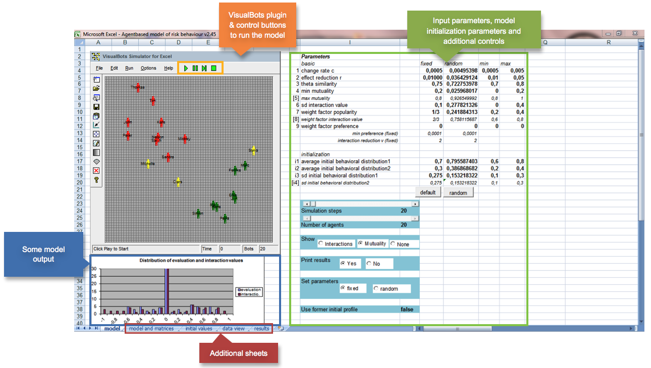
Figure 1. Screenshot of the models' graphical user interface. On the left there is the VisualBots plugin (see also figure 2) with the controls (orange box) to run the model. On the right (green box) input parameters can be defined. Some model output is given below the VisualBots plugin (blue box), i.e., distribution of interaction and evaluation values. Further model output is printed out in the results sheet and automatically saved as a separate results file. The "model and matrices" sheet is an alternative way to run the model, i.e. to start a Monte-Carlo-analysis and run several simulations in a row for model validation. The dataview sheet can be used to visually inspect model output and to print graphs. The initial value sheet gives the matrixes/values needed for initializing the model (i.e., initial behavioral profile and preferences). For additional information on the model interface please consult the user manual, which can be retrieved from the model download site (see footnote 1).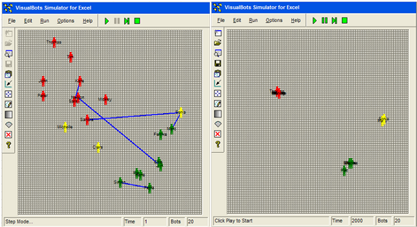

Figure 2. Initial (left: t=1) and final (right: t=2000) screenshot of the simulation model VisualBots GUI. The figure shows the agents on the behavioral state space with the x axis indicating conventional behaviors and the y axis indicating risk behaviors. Colors indicate the type of behaviors (green: conventional agents; yellow: mixed behavior; red = risk behavior prone agents). The figure on the left shows the beginning of the formation of the network (i.e., start of the simulation t1). Blue connection lines indicate an interaction between the two corresponding agents. The agents change their behavioral profile on the basis of the interactions. The figure at the right shows the end of the simulation, in which three agent clusters appear with similar behavioral profiles.

General Procedure and Simulation

2.6

A model run covers 2000 simulation steps representing 200 days approximating one school year and 20 agents representing a school class. In every simulation step the different property matrices are updated. Ten simulation steps shall represent a school day, 50 a school week and 200 steps a month. Each agent can interact with each other agent during one simulation step, so every agent has a maximum number of 19 (= number of agents -1) interactions per simulation step. Correspondingly, during a school day an agent has the opportunity for 190 interactions (simulation steps per day = 10 × number of agents-1 = 19). We assume that we start the simulation at the beginning of the school year. The class is newly formed; the agents have never met before.

An updating cycle and model initialization

2.7

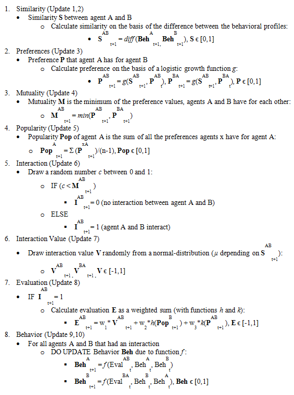
The simulation consists of successive steps during which the properties are updated. Figure 3 shows all major properties of the model and indicates the model updating cycle within the simulation. The updating cycle describes all calculations conducted for one simulation step. The circles indicate the different properties of the agents. The boxes contain the model parameters and thresholds (which can either be set to a fixed value or calculated as an average). The calculation rules for the agents' properties will be introduced in more detail in the "Formal model" section (see formulas 1-6). Furthermore, figure 3 gives an impression of how the model states are interrelated and connected to each other indicated by the arrows. The dashed arrows denote an influence by a parameter or threshold. The solid arrows report the influence between the agents' properties.

2.8

Before starting a model run and the calculations for the first simulation step, behavioral and preference values have to be initialized. The behavioral profiles are initialized on the basis of random values drawn from two different normal distributions. The initial preference values are random values between 0 and 1 (see appendix C and web materials for further details on the model initialization).

2.9

The first two computations during a simulation cycle (a step in the model) are the updates of the similarity and the perceived similarity (update 1 and 2, yellow). As soon as the perceived similarity is updated, the growth rate for the preference and consequently the new values for preference can be calculated (update 3, blue). The values for mutuality as well as for popularity are refreshed on the basis of the new preference data (update 4 and 5, blue). After the determination of the mutuality values, the decision can be made whether two agents interact or not. Additionally, the value for these interactions is calculated (update 6 and 7, green). The updating cycle proceeds with the evaluation of the interactions (update 8, violet). As can be seen from figure 3, evaluation depends on many factors that have to be determined first. Therefore, the evaluation is calculated as one of the last states within the simulation cycle. The final updates consist of the calculation of the behavioral change due to the results of the evaluation and the change in the perception of the other agents' behaviors (update 9 and update 10, light green).

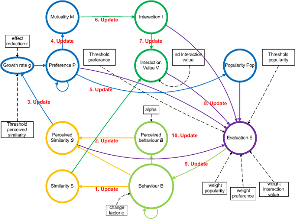
Figure 3. Model overview and updating cycle. The figure shows the main properties of the model and additional parameters. The arrows indicate the influences between the different properties. Numbers 1 to 10 show the sequence of updates within the model.

Model output & Data Inspection

2.10

Simulated longitudinal data are stored and exported as comma separated result files. The results files contain all simulated data (i.e., behavioral profiles, similarity matrices, preference matrices, mutuality matrixes, interaction matrices, interaction value matrices, evaluation matrices, popularity values) and are the basis for further analyses. All result values are real numbers (double values) between 0 to 1 (behavior, similarity, preference, mutuality and popularity) with 1 indicating a maximal possible occurrence of the corresponding property. Other variables vary between -1 and 1 (interaction value, evaluation) with values from -1 to 0 indicating negative interactions/evaluations and values from 0 to 1 representing positive interactions/evaluations. For some illustrations of the model output matrixes see figure 4.

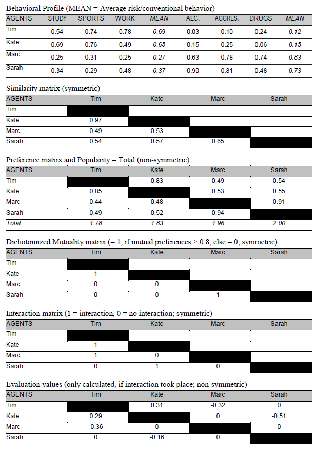
Figure 4. Typical output matrixes for a simulation step (simplified examples of 4 agents).

2.11

Simulation data can be visually inspected, i.e. by plotting graphs and developmental curves of these different properties over the simulation on the basis of the exported data (e.g., see figure 5 for a graph showing the development of risk behavior). Emerging friendship networks are calculated on the basis of the mutuality values and illustrated with NetDraw^[2] (a software for visualizing and analyzing social network data; Borgatti, 2002; see also figure 6 and 7), additionally allowing for a first (visual) inspection of the emerging friendship networks and the different roles/positions of the agents within the network. Furthermore, NetDraw offers some rudimentary functions to analyze social network data. In addition, the statistical software environment R (R Project 2013) is used to calculate additional measures on the basis of the model output and results file^[3] (i.e., hierarchical clustering of friendship groups in the social network, clustering degree of friendships network, Moran I similarity-proximity measure). These measures and statistics are predominantly used to test the model's validity (see also section "Model validation" for more details).

2.12

The following sections provide an illustration of typical model results. Since the model is based on a stochastic process, e.g., random influences on the interaction occur at every iteration step, model simulations produce a family or distribution of outcomes with certain qualitative characteristics. With the parameter ranges chosen for this example (see also appendix C) we on average receive a network of 2 to 3 groups (see figure 7).

Simulation of the development of risk behaviors

2.13

Figure 5 shows the trajectories of the agents' average risk behavior over time (i.e., mean value of drinking, smoking and aggression; with 1 indicating a maximal value and 0 a minimum value). At about 1600 simulation steps, it seems that two behavioral groups emerge (see figure 5). One group shows moderately low average risk behaviors (about 0.4), the other group has moderately high average risk behaviors (about 0.6). At the beginning of the simulation the variance in the individual levels of average risk behaviors is high (compare the diagram in figure 5 between steps 0 and 200). Over the course of time this variance is decreasing, the agents tend to adapt their behavior reinforcing each other and therefore become more and more homogenous (see around step 1600). A special case is Jan, who had an initial low value for average risk behaviors, but was not reinforced by all the other low-risk agents having low risk behaviors. Instead, he has been attracted or influenced by the more risky agents, and increases his risk behaviors.

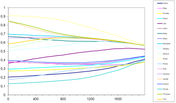
Figure 5. Development of average risk behaviors. The figure shows the development of the average risk behavior for the 20 agents in the model simulation (x-axis indicates simulation steps, y-axis indicates value for average risk behavior). Average risk behavior is calculated as the mean of the different risk behaviors (i.e., alcohol, aggressiveness, soft drugs).

Friendship network development

2.14

After the first day at school, when the agents have met for the first time, preferences and mutual preferences are formed. A friendship connection is defined as one that corresponds with a mutuality level > 0.8. Figure 6 shows the social network after the first day at school (t = 10).

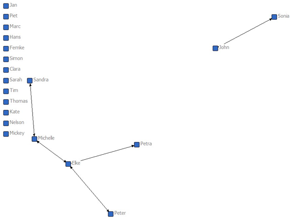
Figure 6. Friendship network (t = 10), showing many isolates and only a few initial friendship connections. The graph is a visualization of the mutuality matrix made with Netdraw (Borgatti 2002). A friendship connection indicates a mutuality value > 0.8.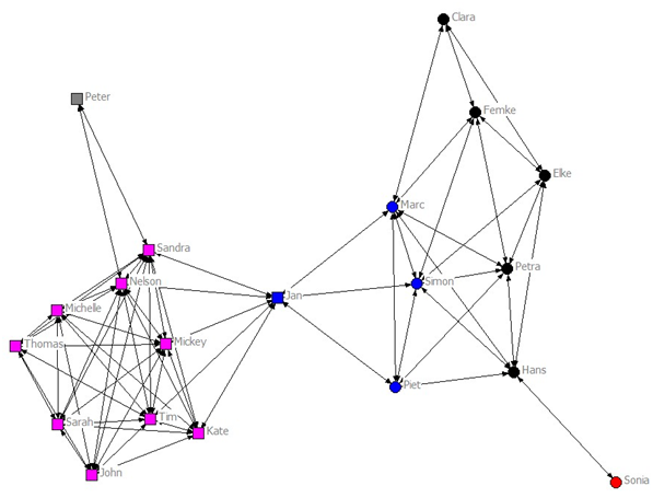

Figure 7. Emerging friendship network (t = 2000). The different colors indicate different clusters. See text for further explanations.

2.15

Figure 7 shows the complex social network after 2000 simulation steps, consisting of two groups (left and right). In general, the majority of the agents in the network are integrated in a group with multiple connections to the different group members. Jan owns a special position, namely that of a liaison (Ennett & Bauman 1996), as he connects the members of two disparate groups. Sonia and Peter have only very few friendship connections. Without her connection to Hans, Sonia would be isolated. Although Peter has two reciprocal friendships (one to Sandra and one to Nelson), he is not integrated in the friendship group. Ennett and Bauman (1994, 1996) define cliques as a small group of at least three adolescents closely connected with each other. Isolates are non-members of a clique (but they may have relatively few friendship connections and still be part of the overall social network). Given our definition that an adolescent is isolated if he or she has less than three friendship connections, Sonia and Peter are isolates in the current network. Furthermore some agents seem to hold a more central role than others, since they have got more connections with others: they can influence more agents, but can also be influenced by more agents than the less central agents (Sandra and Nelson in case of figure 7).

Friendship groups and behavioral homogeneity

2.16

How are friendship formation and development of behavioral profiles interrelated? In the current network, two major groups have emerged. A hierarchical cluster analysis of the mutuality matrix at t = 2000 shows how the position in the social network and behaviors are associated. A circle displays that the agent has an average risk behavior smaller than 0.5 and an average conventional behavior bigger than 0.5. The square means that the agent has an average risk behavior bigger than 0.5 and an average conventional behavior smaller than 0.5. The colors denote the different clusters of preference (see figure 7. The cluster analysis recognizes Peter and Sonia as isolates too. The cluster analysis discriminates between a risky group (pink squares left) and a conventional group (blue and black circles right). Jan belongs to the blue cluster right, though he shows more risk than conventional behavior (indicated by the square).

The formal model

3.1

On the basis of a comprehensive literature review Ballato (2012) developed a conceptual model on the development of (risk) behavior in social groups in adolescence (for a detailed description of this work see also Ballato 2012, chapter 2), which built the basis for our formal mathematical model. The basic elements and mechanisms of this model are shown in figure 8. The agent-based model, the agents' properties and the functional relations between these properties were all based on the central properties and mechanisms described in this conceptual model.

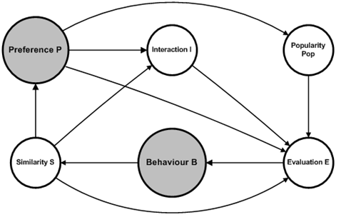
Figure 8. Conceptual framework (based on Ballato 2012).

Behavior and perceived behavior

3.2

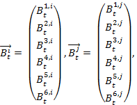
The property "behavior" is a list of behaviors used to specify an agent's behavioral and habit profile. It consists of both conventional and risky behaviors. Every agent possesses an individual behavioral profile, which consists of three different types of risk behavior (i.e., aggressiveness, alcohol abuse and abuse of soft drugs) and three different types of conventional behavior (i.e., engagement in sport activities, attitude towards work and attitude towards studying). Each behavior B has an index k ∈ (1, 2, 3, 4, 5, 6), so we have:

Bk

with k = 1 indicating study, k = 2 indicating sports, k = 3 indicating work, k = 4 indicating alcohol, k = 5 indicating aggressiveness, k = 6 indicating soft drugs.

3.3

This profile is updated over the course of time in the simulation. B_t^k,i indicates behavior k of agent i at time step t, t ∈ (0, 1, 2, …, n), n = number of iterations. An agent's level of involvement in a particular behavior is represented by a number that varies from zero (it does not occur) up to a level of involvement of 1, which corresponds with the maximal frequency of occurrence of that behavior in a single agent in the population of interest. Hence, B_t^k,i ∈ [0,1]. The new behavior k value of agent i at time t+1 is calculated as a function of his former behavior k at time t. This function additionally takes the behavior k of all the agents j into account, with whom agent i had an interaction. The magnitude of change also depends on how positively (or how negatively) agent i evaluated the interactions with the other agents. In formula:

(1.1)

with

and n = number of agents, c = change rate parameter, defined as the evaluation of an interaction with agent j (see also formula 6)^[4].

The perceived behavioral profile

3.4

Every agent has a subjective perception of all the other agents' behaviors. This subjective perception is called the agent's perceived behavior. The behavior k that agent i perceives from agent j is calculated on the basis of a distortion of agent j's real behavior. This distortion is initially randomly chosen (from a normal distribution) and decreases over the course of time. The theoretical justification for this assumption is that over the course of time the agents in a school class communicate and interact with each other and obtain more and more information about the real behavioral profile of the classmates. In a formula we can describe this like follows:

(1.2)

with
and indicates behavior k that agent i perceives from agent j for the time step t+1, indicates agent j's real behavior at time step t, α can be used to manipulate the amount of time agent i needs to perceive the real behavior of agent j, α > 0, is a normally-distributed random variable with standard deviation sd_{initial perceived behavior} and mean set to .

Similarity and perceived similarity

3.5

Every agent has a certain similarity with the other agents depending on how similar his or her behavioral profile is with the behavioral profile of another agent. This similarity is calculated on the basis of the difference between the six-dimensional behavioral profiles of the corresponding two agents. In terms of a function we can define:

(2)

with

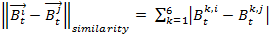
and

m = 6 (= number of behaviors), i ≠ j.

3.6

If the similarity is calculated like shown in formula (2), the similarity value has to be within the range of 0 to 1, so for all t ∈ {1, 2, …, n}, with n equals the number of iterations.

The perceived similarity

3.7

The perceived similarity is based on the subjective impression of the behavior of the other agents (i.e., the perceived behavior) instead of the real behavior. Consequently, there must also exist a subjective impression of the similarity. An agent feels similar to another agent on the basis of what he thinks is the other agent's behavior. This perceived similarity is therefore computed like in formula (2), but using the perceived behavioral profiles of the OTHER agents instead (and NOT their real behavioral profile).

Preferences

3.8

The preference indicates how much agent i likes agent j at time step t. The value for the preference can vary between 0 and 1, so . The preference is calculated as a logistic function with a growth rate g_t that depends on the perceived similarity. For g_t > 0 the capacity limit for the preference is 1. When an agent reaches the capacity limit, it means that he maximally likes the other agent. For g_t < 0 the capacity limit is 0, which means to absolutely dislike another agent ^[5]. The preference is calculated as follows

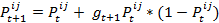
(3)

with

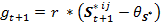
Parameter r, with 0 < r < 1, moderates the effect of the perceived similarity on the growth of the preference. θ_S^* is a threshold that is set to a fixed value between 0 and 1, so θ_S^* ∈ [0, 1].

Mutuality

3.9

Mutuality indicates how much two agents mutually like each other, and is thus tightly connected to preference. The model takes the mutuality value as an indicator for friendship, as friendship necessarily implies a certain mutuality in terms of preference, i.e., there must be mutual preference, or shortly mutuality. Therefore the rule for calculating the mutuality value is to simply take the lowest of the two preference values that two agents have for each other:

(4)

gives the mutuality between agent i and j at time step t+1.

Popularity

3.10

The property "popularity" is the sum of the preferences of all the agents for another agent. It is calculated by dividing the sum of the preferences by the number of agents n - 1. Therefore every agent in the model possesses a certain popularity value within the range [0,1]. The agents express a real preference for the other agents; thus, the model employs a socio-metric notion of popularity. The popularity value Pop of an agent i at time t+1 equals:

(5)

with i ≠ j, n = number of agents.

Interaction and Evaluation

The interaction frequency

3.11

In a class or during a school day a lot of interactions take place, whether in the bus on the way to school, during lessons or during the break on the school yard. Some of these interactions are compulsory, for example, if the teacher has decided that Jan and Piet have to work together on a math problem. We assume that most of the interactions at school are voluntary. The agent's free decision to interact or not to interact with another agent depends on the one hand on how much this agent likes the potential interaction partner and on the other hand on additional random influence. This random influence shall represent the possibility that two agents do not necessarily have to interact all the time because they have a high mutual preference. For example, although two persons A and B might be best friends, sometimes person A wants or needs to say something to someone else. Or on the other hand, although a person does not like a fellow student, the teacher might force him/her to work together with this person on a specific task, or there are other reasons requiring an interaction. In order for an interaction to take place it is not only important that agent X likes agent Y, but also that agent Y likes agent X. For example, Jan can like Piet very much, but if Piet has no interest in Jan and avoids him, there will hardly be any interaction. The mutuality and randomization requirements are combined by drawing a random number between 0 and 1 from an equal distribution. If this number is smaller than the mutuality value , the interaction takes place ( = 1), else not ( = 0).^[6]

The interaction value

3.12

An agent can have a positive or a negative impression of an interaction, i.e., feel positive or negative about a particular interaction. This impression of course can differ between the two interaction partners. If Jan and Piet have an interaction, Jan may have a very positive feeling about this, whereas Piet might have a moderate positive feeling about the interaction. In general it is also possible that one agent evaluates an interaction negatively, but the interaction partner evaluates the same situation positively. This is typical of a bullying interaction, but we shall assume that overall it represents an infrequent situation.

3.13

The interaction value is drawn randomly from a normal-distribution with mean (μ ∈ [-1, 1], similarity threshold θ_S^[7]) and the standard deviation σ_V = sd_{interaction value} (fixed predefined value).

Evaluation

3.14

The evaluation represents the important process of deciding how an agent personally evaluates the interaction with another agent: Positively or negatively? Based on the literature, we assume that this decision does not only depend on the content of the interaction, but also on the popularity and the similarity of the interaction partner as well as on the preferences for the partner. Evaluation is the process of taking all these factors into account, weighing them and making a final decision on the question: How do I presently evaluate the interaction we just had? The rule for calculating this evaluation is as follows ^[8]:

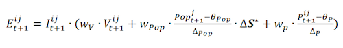
(6)

with

Model validation

4.1

In the following sections we propose different hypotheses to determine the validity of the model. The hypotheses are formulated on the basis of research results in the area of adolescence development (see Ballato 2012, chapter 2, for an extensive review). In the final section, the methods for testing these hypotheses are explained (for detailed descriptions see also appendix B).

Group formation hypothesis

4.2

Friendships in adolescence are mainly organized out of dyadic relationships. The dyadic relationships then interlink with each other to form more complex groups of friendship relations, mostly referred to as cliques and crowds (Brown & Klute 2003; Ennett & Bauman 1994; Hallinan 1979) ^[9]. A considerable amount (up to about 50%) of adolescents in school are member of a clique (Cohen 1977; Coleman 1961; Ennett & Bauman 1994, 1996; Hallinan 1979; Hallinan and Smith 1989; Kandel 1978). Consequently a major feature of the model should be that it is able to represent the emergence of such groups.

4.3

Using classical hypothesis formulation our first hypothesis is: H₁: The model reveals emergence of distinct friendship groups. The null hypothesis is: H_0,1: The model reveals no emergence of distinct friendship groups.

Homogeneity hypothesis

4.4

Researchers have often investigated the homogeneity in dyadic friendships and friendship groups (Byrne 1971; Cohen 1977; Ennett & Bauman 1994, 1996; Kandel 1978). Adolescents tend to be similar in their conventional behaviors as well as in their risk behaviors. Many researchers have studied homogeneity tendencies in risk behaviors. Schulenberg and Maggs (1999) focused on peer influences on drinking behavior; Espelage et al. (2003) on homogeneity in aggressive behavior; Ennett et al. (1994) studied homogeneity in smoking behavior; Patterson and Dishion (1985) investigated homogeneity in delinquent behavior and Kandel and Davies (1991) focused on homogeneity in illicit drug use. The findings on homogeneity in conventional behaviors are similar. Henrich et al. (2000) found considerable homogeneity for school adjustment. Jessor et al. (1998) found that peers who model conventional behavior tend to be a protective factor for a particular adolescent's own health behavior.

4.5

In line with these theoretical findings, our model should be able to simulate and explain a connection between the distance or closeness between the agents in the friendship network and their behavioral profile, indicating that agents standing closer together in the social network (i.e., being friends) also tend to have similar behaviors. The second hypothesis and null hypothesis are: H₂: The model reveals a relationship between the behavioral attributes and distance between friends in the social network (small distance-high behavioral similarity). H_0,2: The model reveals no relationship between the behavioral attributes and distance between friends in the social network.

The hypothesis on the behavioral change dynamics and the emergence of homogeneity

4.6

It is assumed that agents change or adapt their behavior faster in the beginning than at the end of the simulation. Empirical findings indicate that the change in homogeneity in established friendships is lower than comparable changes in non-stable friendships (i.e., friends to be at time 2). Kandel (1978) showed that adolescents who would become friends in the near future showed a greater change in their frequency of marijuana use, their educational aspirations and minor delinquency than compared to adolescents in established stable friendships. Bot et al. (2005) found that the change in drinking behavior was lower in established and reciprocal friendships than in unilateral friendships. The explanation is that, because mutual friends already have got a high level of similarity, the behavioral change by influencing each other is relatively low.

4.7

In summary, we expect that group members have changed their behaviors more in the beginning than at the end of the simulation. Therefore, the decrease of the behavioral variance (within a group) should be faster in the beginning than in the end: H₃: The model reveals a difference between the initial and final decrease of behavioral variance within the groups. H_0,3: The model reveals no difference between the initial and final decrease of behavioral variance within the groups.

Influence and reinforcement hypotheses

4.8

In addition to similarity as a major factor for selection of friends, peer influence has also been an important focus of research in adolescents.

4.9

In line with Kandel's (1978) pioneering work, recent research has shown that homogeneity can best be explained on the basis of the processes of similarity as well as influence and reinforcement (Burk et al. 2007; Engels et al. 1997; Hoffman et al. 2007).

4.10

The model defines influence or reinforcement in general as a behavioral change due to an interaction with another (peer) agent. The agents adapt their behavioral profile towards the behavioral profile of another agent, if they have a positively evaluated interaction with each other.

4.11

More specifically, "reinforcement" refers to changes in behavior, indicating that the peers actually reinforce the behavior of others without being directly exposed to a certain pressure, implying that reinforcement is a reciprocal process. These changes are mostly small (short-term) changes in frequencies or intensities of behaviors based on the evaluation of the interactions. The agents adapt to the average behavioral profile of the peers within their friendship-network or "clique" (e.g.. adapt from smoking 15 to 20 cigarettes per day). "Influence" implies that an agent is changing his or her behavior in a somewhat discontinuous way (in a long-time perspective) and in fact adopts new behaviors. For instance, an agent initially shows a behavioral profile that is closer to the average behavior of a "clique" A (e.g., a non-smoker group), but then the agent becomes a member of "clique" B (e.g., consisting of smokers) and starts to smoke. The transition to smoking is an effect of influence.

4.12

The hypothesis and null hypothesis for the influence process are: H₄: The model generates cases of influence. H_0,4: The model generates no cases of influence.

4.13

Most of the time, most of the agents will actually not be influenced, but be reinforced, thus stabilizing their behavior within a corresponding group of similar agents, which corresponds with the following hypotheses H₅: The model will generate reinforcement for a majority of cases. H_0,5: The model will not generate reinforcement for a majority of cases.

Procedure and data analysis methods

4.14

For each hypothesis presented above, a specific method for testing has been used. These methods are partly adopted from SNA and are not always common in classical psychological analysis. They will be explained in more detail below.

4.15

In order to compensate for chance variation, we executed 100 model runs (each consisting of 2000 simulation steps) and analyzed the corresponding model results. This number represents a good compromise between the limit of the computational resource and the reliability of the model (see also appendix B). At the beginning of each model run, parameters were randomly drawn from an equal distribution over a corresponding parameter range. The ranges were defined either based on empirical findings or estimated on the basis of theoretical considerations or the modelers' experience from several model test runs (see table 1 and appendix D for a detailed description of the parameter ranges and their estimation). In principle, we decided on default parameter values and ranges that result in "acceptable" behavior of the model over a number of iterations chosen to represent a realistic time course. Starting from these workable parameter values, we were then looking for differences in parameter values that produce certain types of behaviors and evolutions of the system that are consistent with the empirical data or the qualitative, conceptual predictions. In other words, we conducted a screening in advance by systematically varying single input parameters to observe overall model behavior (i.e., distributions, ranges, and dynamics of model output). By doing so, we found suitable parameter ranges for the input parameters. For example, if the input parameter c (change rate) is set to values > 0.005 this leads to a tremendous change in agents' behaviors (i.e., going from wallflower to super-risk agent within 10 simulation steps). On the other hand, if c is < 0.0005 we observe hardly any behavioral change in the agents' within 2000 simulation steps ( = one school year), which is an unrealistic output as well.

4.16

Finally, the results of the 100 model runs were used to check if an observed phenomenon (e.g., the building of friendship groups) is just due to an accidental sample or really a qualitative property of our model (e.g., by using Monte Carlo simulation techniques; see also Steenbeek and van Geert 2008).

Table 1: Parameter settings for model validation.
Parameter	Range/default	Further explanations
	Min	Max
c	0.0005	0.005	The change rate c can be used to modify the dynamics of the behavioral change (i.e., the higher this rate, the faster the behavioral change). The parameter range was defined on modelers' experience. Generally, values > .005 led to a unrealistic rapid change in agents' behaviors and values < .0005 result in almost no behavioral change. See also formula 1.1.
r	0.01	0.05	The effect reduction parameter r reduces the magnitude of the increase in preferences. The smaller the value, the higher the reduction. We estimated the parameter range based on a longitudinal study empirically describing friendship formation in school classes (Hallinan 1979). See also formula 3.
θS	0.7	0.8	The "true" similarity threshold is used to calculate the interaction value. If the similarity is below the threshold, the probability of a positive interaction is predominantly low, and vice versa. See also section "The interaction value".
minM	0.0	0.2	Minimum/Maximum value of mutuality (with maxM = 1 − minM). If the mutuality value is smaller (bigger) than min (max) mutuality, it is set to min (max) mutuality. Parameter ranges are defined on the basis of theoretical considerations. Min/max mutuality influence the decision whether an interaction between two agents takes place or not (see also section "The interaction frequency"). Generally, these parameters guarantee that it is possible for the agents to interact with disliked others and to pause interacting with friends.
maxM	0.8	1.0
σV	0.0	0.4	On the basis of theoretical considerations we defined a standard deviation value of 0.2 as a default value. Thus, a parameter range from 0.0 (no deviation) to 0.4 (moderate deviation) is appropriate here.
wPop	0.2	0.4	Parameter ranges for the weight factors were defined on the modelers' objectives and theoretical considerations. Ranges can be varied to test different assumptions and to compare different scenarios (e.g., a scenario with a high impact of popularity on the evaluation vs. a scenario with a high impact of the interaction value). As a constraint the sum of all weight factors has to be one. For the model validation we have parameter settings of a scenario, in which the interaction value has a stronger impact on the evaluation than the popularity value and the influence of preference is not taken into account.
wV	0.6	0.8
wP	0
minP	0.0001		Minimum value of preference. If the preference value gets smaller than min preference, it is set to min preference. The parameter is a static default value.
v	2		The parameter regulates the overall interaction frequency (i.e., values > 1 reduce the number of agents' interactions in the model; see also section "The interaction frequency"). The parameter value is a static default value.

Group formation & Clustering degree

4.17

For testing hypothesis 1 (group formation), we used the clustering coefficient, originating from SNA. This coefficient measures the tendency of a network to build dense local neighborhoods, i.e., "clustering" or group formation (for further explanations see appendix B). According to our null hypothesis the clustering degree should be 1 or zero, that is, either the local network density and the overall network density are the same, so no tendency of building distinct groups in the data is given, or, all agents are isolated or only isolated dyadic friendships exist, so actually no friendship groups emerged.

Homogeneity & Proximity-similarity measure

4.18

For testing the second null hypothesis (homogeneity), a statistic originating from geography is used: The Moran "I" spatial autocorrelation statistic (also referred to as Moran "I" proximity-similarity statistic; Esri 2012). This statistic ranges from a value of 1 indicating high correlation, between proximity and similarity in the network, through 0 indicating no correlation, to the value of -1 indicating negative correlation. In geography this statistic is used to check the extent to which the similarity of the geographical features of any two places is related to the spatial distance between them (e.g., whether you find a certain kind of fauna only in certain areas). Adapted to social network analysis we would like to check whether the distance between agents in the network is correlated with some of their attributes (e.g., if agents close together in the network show similar behaviors).

Behavioral change dynamics

4.19

To check hypothesis 3 (behavioral change dynamics and emergence of homogeneity) the following two step process is carried out. First, an agglomerative hierarchical cluster analysis^[10] is conducted for each of the 100 model results to define the different friendship groups and its members that have emerged at the end of a simulation (t = 2000). Friendship clustering is based on a dissimilarity matrix (which is calculated on the basis of the mutuality matrix at t = 2000). An a priori number of four groups is assumed, so the four biggest clusters are actually given. If a cluster has less than three members, it is not included for further analysis.

4.20

Secondly, we compared the change in behavioral standard deviation at the beginning with the change in behavioral standard deviation at the end of the simulation (indicated by ΔSD; see appendix B for details). To evaluate the statistical significance of ΔSD we use the bootstrap (resampling) technique (Moore & McCabe 2006) ^[11].

Influence and reinforcement

4.21

To check the final null hypotheses (influence and reinforcement), the following analysis method is applied: First an agglomerative hierarchical cluster analysis has to be conducted to define friendship groups within the social network of the class at the end of a simulation (t = 2000) with clusters formed on the basis of a dissimilarity matrix. Groups with less than four members are excluded from further analysis. On the basis of the cluster analysis we thus receive n different groups (for simulations with 20 agents n is between 2 and 5). For each of the n different groups, a typical initial behavioral group profile is calculated retrospectively (on the basis of the average individual behavioral profile of all group members, that they have shown at the beginning of the simulation, i.e., at t = 10). In other words, we receive a typical initial behavioral profile, which is representative for agents that finally become a member of group X at the end of the simulation (called "typical initial group X profile").

4.22

If the initial individual behavioral profile of an agent A (consisting of the average conventional and risk behavior) is similar to the "typical initial group X profile" and agent A actually becomes a member of group X at the end of the simulation, we define this as a case of reinforcement (slow coadaptation of agent A and the members of group X). If agent A finally ends up as a member of group Y (though agent A's initial profile is actually more similar to typical members of group X than Y) we define this as a case of influence (agent A gets attracted by members of group Y and finally adapts to the behavior of the group members Y).

Results

Group formation (clustering degree)

5.1

In 12 cases of the 100 model runs the overall density was the same as the clustering coefficient: The degree of clustering was 1 (see figure 9). In these cases a maximal network emerged, where every agent was connected to all other agents. In none of the cases all agents have been isolated at the end of a simulation (clustering coefficient equals 0). Most of the simulation results yielded a moderate degree of clustering, on average the local neighborhood density was about double the size of the overall density (M = 2.14).

Figure 9. Frequency distribution for the different values of the clustering degree. Values for the clustering degree between 2 and 2.5 are most frequent (50 times).

5.2

On the basis of these simulation results the first null hypothesis must be rejected. The observed probability of building groups (i.e., clustering degree > 1) is .88 (88 cases out of 100 model runs), which is significantly different from the expected probability p = 0 (binomial- test: p < .001). But, how well does the model represent group formation? If we choose a clustering degree of 1.6 as a cut-off value indicating a moderate degree of clustering, we have 69 cases (clustering degree > 1.6) out of 100 model runs. With a confidence of 95% the model reveals results with a clustering degree indicating moderate to higher levels of distinct group formation with a probability p between 59.01% and 77.84%.

5.3

An alternative explanation is that the clustering degree was present from the beginning of the simulation. A permutation test (1000 runs) reveals a highly significant difference between the average clustering degree at the beginning and the average clustering degree at the end (p < .001), which thus contradicts the alternative explanation.

Homogeneity (proximity-similarity measure)

5.4

In order to check a possible interrelation between the behaviors and closeness in the friendship network the Moran "I" proximity-similarity statistic was applied to the 100 simulation results. On average the Moran "I" between average risk behaviors and closeness in the, network was .76. In most of the cases the Moran "I" proximity-similarity measure lay between .80 and 1.0 (see also figure 10).

5.5

In 87% of the cases the Moran "I" proximity-similarity statistic between the average risk behaviors and the closeness in the friendship network was significantly different from 0 (α < .05; random permutation test). The 95% confidence interval for the expected p-value (of having meaningful or significant correlations between proximity and similarity) lies within 78.80% and 92.92%. Similar results can be found for the comparison with average conventional behavior (88% significantly different from 0, α < .05). The 95% confidence interval for the true success probability p is between 79.98% and 93.64%. On the basis of these results also H _2,0 has to be rejected.

Figure 10. Frequency distribution of the Moran "I" proximity-similarity values for average risk behavior (100 model runs).

Behavioral change dynamics (ΔSD )

5.6

In order to check H_3,0, ΔSD (indicating the change difference of the behavioral standard deviation) has been calculated for the 100 model runs (see figure 11). In 23% of the cases ΔSD is smaller than or equal to zero. In 77% of the cases ΔSD is bigger than 0 (M= .0271, SD = .0263). For the average conventional behavior, in 24% of the cases, ΔSD is smaller than or equal to 0, in 76% of the cases it is bigger than 0 (M= .0261, SD = .0253).

Figure 11. Frequency distribution of ΔSD for average risk behaviors.

5.7

Bootstrapping results indicate that the 95% confidence interval for ΔSD is between values .0235 and .0309. Because 0 is excluded from the interval, ΔSD is significantly different from 0. In other words, in the model the decrease in behavioral variance within the groups is stronger at the beginning than at the end of the simulation. Null hypothesis H_3,0 can thus be rejected.

Influence and reinforcement

5.8

For the average risk behaviors, results from the 100 model runs (100 model runs × 20 agents = 2000 cases) revealed influence in 102 cases (5.1% of all cases). In 272 cases (13.6% of all cases) agents were not a member of a group or member of a group with less than 4 members. This means that no group was formed at all. As already mentioned above, these agents have been excluded from the analysis of influence and reinforcement. The majority of the agents were reinforced in their average risk behaviors (1626 or 81.3% of all cases). In 29 model runs we receive at least one case of influence (so the amount of influenced agents in 29 out of 100 model runs was 1 or bigger). In 97 out of the 100 model runs we obtained 10 or more cases of reinforced agents. For the conventional behaviors the results show a similar picture: 101 cases of influence (5.05%), 1627 cases of reinforcement (81.35%) and 272 (13.6%) excluded cases. In 98 out of the 100 model runs we have 10 or more cases of reinforcement; in 31 runs we receive at least one case of influence (see table 2).

Table 2: Averages and standard deviations for influence and reinforcement cases in average risk and average conventional behaviors (possible value-range: 0 to 20 agents).
		Risk behaviors	Con. Behaviors
Influence	M	1.02	1.01
	SD	2.2	2.09
Reinforcement	M	16.26	16.27
	SD	2.16	2.06

5.9

This table shows that the probability for having one case of influence or more within a simulation run is significantly different from 0 (average risk behaviors: p < .001, average conventional behaviors: p < .001). Therefore, H_0,4 (i.e., the model gives no cases of influence) has to be rejected. Also H_0,5 (i.e., the model will not represent reinforcement for a majority of cases) has to be rejected (if we define majority as more than 50% of the agents). The probability of seeing at least ten or more cases of reinforcement (of 20 agents) in a simulation result is significantly bigger than p = .50 for average risk behavior (p < .001) as well as for average conventional behavior (p < .001).

Summary and conclusion

6.1

To recapitulate, the model has two closely related aims. First, it should have explanatory power, and second it should be able to generate typical qualitative properties found in empirical research. These qualitative properties refer to various empirically supported hypotheses, three concerning the concept of homogeneity, two dealing with the concept of influence and reinforcement.

6.2

As regards the first hypothesis, the results show that the model demonstrates the formation of distinct friendship groups with different degrees of clustering. On average two dense clusters (or friendship groups) emerge. In addition, the model can produce a spectrum of emerging social networks. This variability is also a characteristic of real emerging social networks (Ennett and Bauman 1996). A potential problem of the model might be that in 20% to 40% a tendency to build one big cluster occurred. This seems to be not always the case in a classroom (e.g., according to Hallinan (1979) about 50% of adolescents on average are not part of a friendship clique). It is possible that this empirical finding is due to the fact that the real adolescents have many contacts with adolescents outside their classroom (e.g. church influence and religious group activities, neighbourhood, sport clubs, music groups and various free-time activities). The existence of the variety of contacts could to a certain extent, "protect" them from being influenced by peers in the classroom, for instance if they already have strong friendship bonds with peers outside the classroom.

6.3

As regards the emergence of homogeneity among friends and groups of friends, the results for the correlation between distance in the friendship network and the behavioral profile clearly support the hypothesis that agents standing closer together in the network also tend to behave more similar and those with higher distance in the network seem to be more dissimilar. However, in some cases one big homogenous group emerged^[12], which in reality is quite unlikely. To avoid this overclustering-effect the model should be adapted and additional parameter settings could be tested. However, the general simulation result of increasing and stabilizing homogeneity among friends corresponds with the empirical data.

6.4

The third hypothesis, postulating that the model reveals the empirically predicted differences between the initial and final decrease of the behavioral variance between the groups could be supported. In terms of an underlying process, this could mean that we have found a kind of "discrepancy-proportional peer influence" as explained by Boxer et al. (2005). Friends that are more different e.g., at the beginning of a friendship influence each other more than friends who have an established friendship.

6.5

In case of the last null hypotheses on influence and reinforcement, the model results correspond with reinforcement in most of the cases (about 80% of all cases), and in about 30% of the model runs the results reveal at least one case of influence (or more). The corresponding null hypotheses have thus to be rejected. The model is able to generate a considerable amount of reinforced agents in the model (which means that they adapt to each other by stabilizing their general behavior) as well as cases of influenced agents. Influenced agents tend to be pulled out of their group of origin, consisting of more or less similar agents, into another group of agents who, at the beginning, are different from the influenced agent, who then begins to move in the direction of more similarity with this new group.

6.6

Additionally, the model can be used to experiment in silicio, i.e., to do experiments in the form of simulations (see also Epstein & Axtell 1996). The model can be used as a digital laboratory to test certain system behaviors that can hardly be observed or tested in the real system (i.e., simulating scenarios with a certain number of extremely good or/and bad agents in the model, scenarios including some exceptionally popular agents with high influential power or an outstanding position in the social network in the model, introducing interventions or punitive reactions to extreme behavior, etc.). Thus, new scientific questions can arise from model experimentation, questions that can be answered empirically in subsequent stages of research. Furthermore, it can inspire practitioners (e.g. in pedagogical psychology, social work or juvenile courts) and may have practical implications for questions concerning group dynamics and suitable group compositions as well as possible consequences of the implementation of school based intervention programs.

6.7

In spite of the successes described above, the model clearly has its limitations. To begin with, it consists of an isolated world of adolescents interacting among themselves and not interacting with other adolescents outside the simulated classroom. Second, the behavioral repertoire of the simulated adolescents is relatively poor (6 types of behaviors in all), and all behaviors can occur with equal probability. In the real behavioral repertoire, certain behaviors might eventually conflict with one another, thus reducing the likelihood that they will emerge or increase even if they are highly characteristic of the adolescent's friendship group. Other behaviors might be mutually supportive, such that it is likely that they will increase irrespective of the fact that they are not at all characteristic of the adolescent's peer group. In addition, given higher computational power (e.g. by re-implementing the current model within a different ABM framework than VBA/VisualBots in Excel) additional simulation runs for further qualitative analysis of the model's validity could be conducted, resulting in more refined analyses. In that case, it might also be considerably easier to actually experiment with the effects of different parameter ranges.

6.8

Based on a systemic view (Bronfenbrenner 1979) there are several elements and levels that determine the development of risk behavior during adolescence (i.e., micro-, meso-, exco- and macro-system). For example, at the meso-level peers are one major source of influence (with an outstanding role particularly in youth). But additional elements are important as well, e.g., family context and socio-economic background, structure and affluence in neighbourhood or types of school (Li et al. 2000; Blum et al. 2000). Furthermore, at the micro-level we can find gender and ethnic differences as well, i.e. girls' lower risk taking and boys' "proneness" to risk behavior (Byrnes et al. 1999; Harris et al., 2006). We decided to focus on the most proximate sources of influence as adolescents spend a substantial amount of daytime at school. However, we believe that this choice does not interfere with the quality of the model, since this model is mostly focused on explaining dynamics and much less on explaining factors that influence these dynamics. Furthermore, many of the factors mentioned above actually have an impact on the school or the composition of classes and can be implicitly incorporated in the model. For instance, we can set the agents' initial risk behavior characteristics on the basis of school and neighbourhood properties or the agents' gender. Finally, the reduction of the number of influencing variables is based on a deliberate choice modellers must make in order to establish a compromise between complexity and comprehensibility.

6.9

In short, this article demonstrates that it is possible to use the empirical literature to build an agent model of interactions, interaction evaluation and peer preference. The principles governing these interactions, evaluations and preferences function as "first principles". From these first principles, which are drawn from basic models of agency, a variety of phenomena qualitatively similar to empirical phenomena can emerge, if these principles operate in a dynamic and iterative manner. In this way, these principles explain the empirical phenomena at issue in the way dynamic and agent models habitually do, namely by showing that certain phenomena iteratively follow from a basic series of mechanisms that are different from the phenomena one wants to explain.

Notes

¹ The model and additional web materials (including the model user manual) can be retrieved from http://www.openabm.org/model/3844/version/2.

² NetDraw can be retrieved from https://sites.google.com/site/netdrawsoftware/.

³ The R files used for this article can be retrieved from the additional web materials. The R Software package is available as free software and can be retrieved from http://www.r-project.org.

⁴For calculating the model results in the following sections (model results illustrations and the qualitative analysis) α_ij was set to 0, if 0 < E_t^ij ≤ -1. That means agents did not change their behavior, if there was a negative interaction.The change rate c is a fixed parameter value to speed up or slow down the behavioral change.

⁵ If we would allow P_t^ij to become 0, the preference value would stay 0 and could not recover. To avoid this the preference value is set to a predefined value min preference as soon as P_t^ij < = min preference.

⁶ For calculating the probability of an interaction, we actually use an upper and lower bound for mutuality. If the mutuality value is below min mutuality, it is set to min mutuality here. In general, this assures that though two agents do not like each other, there is still a certain chance for interacting. If the mutuality value is above the max mutuality value, it is set to max mutuality. This guarantees that two agents do not interact all the time in spite of their having a high mutual preference. Furthermore there is a parameter v that controls the general probability of an interaction (with v > 1 reducing and v < 1 increasing this probability).

⁷ The similarity threshold σ_S is used to normalize the similarity values. If the similarity value is below the threshold, the normalized similarity becomes negative, else it becomes positive. If we receive a normalized similarity value bigger than 1, it is set to 1. If the normalized similarity value is below -1, it is set to -1. Therefore we achieve μ ∈ [-1,1].

⁸ Please see web materials for details regarding the evaluation formula and calculation examples.

⁹ For the purpose of this article we used a definition of a "clique", that is somewhat different from the standard definition in adolescence psychology or social network analysis literature (see also appendix B)

¹⁰ The agglomerative hierarchical clustering was conducted with the software package R. Corresponding R scripts with further analysis details are added to the web materials.

¹¹ Under the null hypothesis, the changes at the beginning are statistically indistinguishable from the changes at the end, implying that the standard deviations at the beginning and the end are also indistinguishable. The bootstrap or resampling technique implies that we combine all change values into one set. We then randomly draw observations from this set that we randomly assign to the beginning stage or to the end stage. For each of these randomly sampled sets, we calculate standard deviations and the value of ΔSD. By doing so many times, we arrive at a distribution of ΔSD that characterizes the ΔSD differences we might expect under the null hypothesis (that is, we have bootstrapped the distribution of the measurement error of ΔSD if the beginning or end stages were indistinguishable). By comparing the observed ΔSD with the bootstrapped ΔSD under the null hypothesis, we can determine the probability that the observed ΔSD is due to chance, given the truth of the null hypothesis.

¹² See also web materials for a mathematical steady state analysis of agents' behaviors.

¹³ For the advanced initialization we draw initial values from 4 different normal distributions. Therefore we receive 4 initial populations of agents: risky, semi-risky, semi-conventional and conventional.

Appendix A – Psuedo Code

Appendix B – Further Explanations Methods

Definition of "cliques"

In adolescence psychology literature, the term clique has varying meanings and implications. However, a standard definition is given by Ennett and Bauman (1994): "Cliques have a minimum size of three members. […] Clique members are required to have most of their interaction (>50%) with members of the same clique and at least two links with others."(p. 656). In Social Network Analysis (SNA) a clique is defined as a "maximal complete sub-graph" in a social network, i.e., in a clique all members need to have a tie/connection to all other members of the clique. As many actors as possible are included into a clique, so that all actors have all possible ties present among themselves (Hanneman & Riddle, 2005). The definition of a clique used in the present article leans on these standard definitions, but makes some modifications (e.g., non-overlapping memberships). In order to avoid overlapping membership and to define different friendship clusters, we used a hierarchical cluster analysis (see hypotheses 3, 4 and 5). Overlapping membership means: an agent is a member of different cliques, and not a member of only one clique. For example, the agent can be a member of clique 1 and clique 2, i.e., the agent has an overlapping membership. In a hierarchical cluster analysis every agent belongs only to one cluster/group at the same time. Therefore, we will refer to the term friendship group (or cluster) instead of clique or the term in quotation marks ("clique"). The effect of this approach is that an agent can be assigned only once to a group (or cluster) on the basis of the hierarchical cluster analysis, i.e., he cannot be a member of two or more distinct clusters at the same clustering level. Agents ascribed to the same cluster have similar or equivalent social relationships. To be a member of a cluster, an agent does not need to have a tie to all other members of the cluster, but in general cluster members need to have a similar pattern of relationships. Additionally, the hierarchical clustering gives us the possibility to ascribe agents to a cluster on different levels because small clusters are agglomerated to bigger clusters or units in the analysis. In this sense our definition of a "clique" is "weaker" than the definition in SNA described above and is closely related to the definition used by many adolescence researchers (e.g., Brown & Klute 2003; Ennett & Bauman 1994; Hallinan 1979).

Clustering degree

The cluster coefficient measures the tendency of a network to build dense local neighborhoods, i.e., "clustering". The local neighborhood of an agent A includes all the agents that are directly connected to A. The density of this neighborhood is calculated by the ratio of the present links between all the agents in the neighborhood (leaving out agent A) divided by the number of all possible connections between the agents in the neighborhood. The overall clustering coefficient is then the average of all local neighborhoods of all agents. To accurately interpret this value the overall network density has also to be considered. The overall network density is calculated as the amount of actual ties between the agents in the network divided by the amount of all possible ties in the network. To assess the degree of clustering in the network we divide the overall clustering coefficient by the overall network density (Hanneman & Riddle 2005). The resulting clustering degree shall be a measure for group formation. The clustering degree is calculated on the basis of the dichotomized mutuality matrix6 after 2000 steps representing the friendship network.

Change of behavioral standard deviation (ΔSD)

The change of the behavioral standard deviation at the beginning of a simulation (ΔBehSD_1,2 = BehSD_t1 – BehSD_t2, t1 = 400, t2 = 800) is calculated and compared with the change of the behavioral standard deviation at the end of the simulation (ΔBehSD_3,4 = BehSDt3 – BehSDt4, t3 = 1600, t4 = 2000). The difference in the change of the behavioral standard deviation at the beginning and at the end is indicated with ΔSD (ΔSD = ΔBehSD_1,2 - ΔBehSD_3,4). A positive value ΔSD denotes that the change of the deviation at the beginning is bigger than at the end (i.e., agents adapt their behavior towards "friends" faster in the beginning than at the end of the simulation). To evaluate the significance of ΔSD (i.e., ΔSD is significantly bigger than 0) we use the bootstrap (resampling) technique (Moore & McCabe 2006). We proceed the bootstrapping in the following way: First we resample the data (results of 100 model runs) with the help of PopTools (Hood 2010) and then we check the confidence intervals of the "resampled" ΔSD means.

Appendix C – Parameter Setting for Illustrations and the Analysis

Parameter settings for model results illustrations

Parameter	Value/Range	Constraints and further explanations
General
Iterations	2000
Number of agents	20
Basic
c	0.002
r	0.0175
θS	0.75
minM	0.2
maxM	0.8	with maxM = 1 – minM
minP	0.0001
σV	0.1
v	2
Weights
wPop	1/3
wV	2/3	with wV = 1 – >wPop
wP	0
Initialization
μB1,0	0.7
μB2,0	0.3	with μB2,0 = 1 – μB1,0
σB1,0	0.275
σB2,0	0.275	Is automatically set to the value of σB1,0 (σB1,0 = σB2,0)
Advanced
Enable perceived behavior	false

Parameter settings for qualitative analysis

The parameter values and ranges described below were used to receive the results of 100 model runs for the model analysis.

As a simplification the direct influence of preference on the evaluation has not been taken into account. Therefore the weight factor of preference was set to 0 (w_P = 0). Nevertheless, there is still an indirect influence of preference on the evaluation via popularity and the interaction (the higher the mutual preference, the higher is the general probability for an interaction; the more an agent is preferred, the higher is his or her popularity). Furthermore the perceived behavior (respectively perceived similarity) has been disabled (setting enable perceived behavior = false). That means that the agents can perceive other agents' "real" underlying behavioral profiles/values from the beginning of the simulation (in other words, there is no distortion or uncertainty in their perception of others).

For each new simulation run the parameters are randomly drawn from the parameter ranges with an equally distributed probability (see also web materials for choice of parameter ranges). Some parameters depend on the values of other parameters (e.g., if min_M is randomly set to 0.14, max_M is automatically set to 1 – 0.14 = 0.86).

The preference values are initialized as random values drawn from the range [0,1] with an equally distributed probability. For the initialization of the behavioral profile random values are drawn from two different normally-distributed populations (with σ_B1,0 and σ_B2,0). Correspondingly, we receive an initial population of risky agents and a population of conventional agents (with several agents having an average lifestyle profile with a composition of conventional as well as risk behaviors; see also user manual for more details on the model initialization).

Parameter	Value/Range	Constraints and further explanations
General
Iterations	2000
Number of agents	20
Basic
c	[0.005, 0.0005]
r	[0.01, 0.05]
θS	[0.7, 0.8]
minM	[0.0, 0.2]
maxM	[0.8, 1.0]	with maxM = 1 – minM
minP	0.0001
σV	[0.0, 0.4 ]
ν	2
Weights
wPop	[0.2, 0.4]
wV	[0.6, 0.8]	with wV = 1 – wPop
wP	0	see also text above
Initialization
μB1,0	[0.6;0.8]
μB2,0	[0.2;0.4]	with μB2,0 = 1 – μB1,0
σB1,0	[0.1;0.3]
σB2,0		Is automatically set to the value of σB1,0 (σB1,0 = σB2,0)
Advanced
Enable perceived behavior	false

Appendix D – General Procedure & Choice of Parameter Ranges

General procedure

Seeing our computer model as a "chance" machine, the results that the model produces could be due to an accidental finding or just random influences. In order to avoid these possibilities, we checked if an observed phenomenon (e.g., the building of friendship groups) is just due to an accidental sample or really a qualitative property of our model by using Monte Carlo simulation technique (see also Steenbeek & van Geert 2008). The general logic of a Monte Carlo simulation is as follows: "Using a given data-generating mechanism (such as a coin or die) that is a model of the process you wish to understand [in our case the simulation computer model], produce new samples of simulated data [our model results], and examine the results of those data [what is actually done in our analysis]" (Simon 1997, p. 154). Twelve parameters were randomly drawn from an equal distribution over a corresponding parameter range (that is more or less suitable in order to be able to observe the phenomena we would expect). The ranges were defined either based to empirical findings or estimated on the basis of theoretical considerations or the modelers experience from several model tests runs (see below). These parameters are then used to run a great number of simulations, each of which generates a particular model output. After the model output is generated, the analysis procedure is as follows: For every simulation result the value for the observed phenomenon of interest is calculated (e.g., a value indicating the tendency of building friendship clusters). For these variables of interest further statistical analysis is then conducted. In some cases, a specific form of a Monte Carlo analysis (i.e., permutation test) is used. For significance reasons actually 1000 up to 10000 runs should be made. Due to computational limitations only 100 model runs have been executed and 100 runs were analyzed (one model run took about 9 minutes, 1000 model runs consequently 9000 minutes = 6.25 days). We decided to make 100 model runs because in our view this number represents the best compromise between the limit of the computational resource and the reliability of the model. For results close to statistical significance (e.g., indicating a significance level between 0.15 and 0.05) an additional analysis with more simulations should be made to be able to state the significance of the results. For results clearly indicating the rejection of the null hypothesis (e.g., p < 0.01) or clearly recommending the perpetuation of the null hypothesis (e.g., p > 0.2) it is not expected that performing more simulation runs will actually change the level of (non) significance.

Choice of parameter ranges

A major challenge when developing a model is the question, how to find suitable parameter ranges or settings. The following parameter ranges were defined on the basis of theoretical considerations, the modelers' experience (who had conducted multiple test runs) or on the basis of empirical findings.

1. Change rate (c)

How much does an agent change his or her behavior on the basis of a simulation cycle (agents can have up to 19 interactions per simulation cycle)? This parameter controls the speed of learning of or adapting to the behavior of the other agents (e.g., on the basis of social learning). To find a suitable parameter range for c we have to answer the question: How long do adolescents need (on average) to become homogenous? For example: How long does a non-smoker need, who enters a group of smokers, to adapt his or her smoking behavior to the average group behavior? Or how fast does an adolescent change the average marihuana consume during a school year? Empirical findings to define a suitable range for our parameter c are rare. Therefore, a suitable parameter range was estimated on the basis of model experience. The change rate c is crucial for the behavioral change. A suitable range appears to be [0.005; 0.0005], as values > 0.005 lead to a much too fast change in behavior and values < 0.0005 result in much too small behavioral change.

2. Effect reduction (r)

The effect reduction has an influence on how fast preferences grow respectively decrease. Having a high effect reduction value means that preferences change fast (i.e., they can increase fast or drop fast). To find a suitable parameter range, we need to consider some theoretical assumptions. In general the process of preference formation is quite fast (i.e., within a couple of weeks). To find a lower bound for the parameter range, let us assume that we have got two agents with an initially low preference for each other. But at the same time both agents are quite similar (which is possible in the model). In this case the agents should be able to form a friendship within a school year. Only few empirical findings give information about the exact duration of friendships or non-friendships. Nevertheless, Hallinan (1979) described a longitudinal study on friendship formation in 4 classes of 6th graders and 1 class of 4th graders. For the 6th graders the absence of dyads (friendships) lasted from 189 to 400 days. If we have a look at the logistic growth function of the preference formula (see formula 3 in the article) and set the term (S_t+1^*ij – θ_S^*) to a fixed value, we are able to estimate a suitable parameter range for r. With r set to 0.05, we need 716 simulation steps (or about 72 simulated school days) to receive a preference value of 0.8, given an initial preference value of 0.1 and (S_t – θ_S^*) = 0,1 ∀ t. This is a lower bound for the formation of a friendship with initially low preference. With r set to 0.01 we need 3583 (or about 358 simulated school days) steps to reach a preference value of 0.8 (with same constraints as before). This defines our upper bound for a friendship formation with initially low preference values. Therefore a suitable parameter range for r is [0.01; 0.05].

3. Theta similarity (θ_S)

Theta similarity is used as a threshold to calculate the interaction value. If the (true) similarity is above this threshold, it is very likely that an agent A has a positive interaction with another agent B. If the similarity value is below, it is very probable to have a negative interaction with the other agent. On the basis of several model tests values we can define values between 0.7 and 0.8 as a suitable parameter range for theta similarity.

4., 5. Min mutuality and max mutuality (min_M, max_M)

Min mutuality and max mutuality influence the decision whether an interaction between two agents takes place or not (see also section "The interaction frequency" in the article). If the mutuality value is below min mutuality, it is set to min mutuality. In general this guarantees that an interaction is still possible, even if two agents have a very low mutuality value for each other. On the other hand, if the mutuality value is above max mutuality, the mutuality value is set to max mutuality. This guarantees that an agent A does not permanently interact with an agent B, which he/she likes very much. Suitable values range from 0.0 to 0.2 for min mutuality and 0.8 to 1.0 for max mutuality.

6. Sd_{interaction value} (σ_V)

Sd_{interaction value} indicates the standard deviation for sampling the interaction value. The higher this value, the higher the deviation of the interaction value from the mean interaction value μ, that is defined on the basis of the normalized similarity value (mean (μ ∈ [-1,1], similarity threshold θ_S; see also section "The interaction value" in the article) A deviation value of 0.2 can be defined as a standard value, a range from 0.0 (nearly no deviation) to 0.4 (indicating a moderate deviation) is appropriate for sd_{interaction value}.

7., 8., 9. Weight factors (w_Pop, w_V, w_P)

Parameter ranges for the weight factors w_Pop, w_V, and w_P can be defined depending on the modelers' objectives. Ranges can be varied to test different assumptions, i.e. to compare different scenarios (e.g., a scenario with a major impact of popularity on the evaluation vs. a scenario with a major impact of the interaction value). As a constraint the sum of all weight factors has to be one (w_Pop + w_P + w_V =1). For the parameter settings in the model analysis we developed a scenario, where the interaction value has a relatively strong impact on the evaluation compared to the impact of the popularity value. Still, the impact of popularity should be substantial in this scenario and the corresponding weight factor should have a moderate value. The influence of preference was not taken into account in this scenario (see also appendix C in the article). Thus, we defined w_Pop ∈ [0.2; 0.4] and w_V ∈ [0.6; 0.8].

10. Alpha (α)

Alpha indicates the amount of time needed until an agent A can perceive the real behavioral profile of another agent B. At the beginning of a simulation an agent A has a biased perception of another agent B and his/her behavioral tendencies. The more time the agents spend together at school, the more visible the true behavioral profile becomes. The decrease is exponential (see also formula 1.2 in the article). Alpha can range from 0.0001 to 0.000001. If alpha is chosen within this range, a decrease of an average initial distortion of 0.4 to almost 0 needs (approximately) 300 to 4000 iteration steps.

11. Theta perceived similarity (θ_S^*)

Theta perceived similarity is used for calculating the preference value (see formula 3 in the article). It gives the threshold for an increase or a decrease in the preference. If the perceived similarity value is above theta perceived similarity, there is an increase in preference, else preference drops. Generally the similarity value has to be bigger than 0.5 for an increase in preferences. A similarity value of 0.5 indicates that two agents have (on average) a difference of 0.5 in their behavioral profiles (agent A is 50% "different" from agent B). A suitable parameter range for theta perceived similarity range is 0.7 to 0.8. So an agent A can tolerate (on average) a difference of 20%–30% and still start/increase liking another agent B.

Initialization parameters (basic)

i1-i4. Average initial behavioral distribution, sd initial behavioral distribution (μ_B1,0, μ_B2,0, σ_B1,0, σ_B2,0)

The initial values of the behavioral profiles are randomly drawn from two different normal distributions (for the basic initialization) ^[13]. Therefore we receive two initial agent populations: A risky population and a conventional population (each generally consisting of 10 agents). Empirical findings indicate a moderate negative correlation between risk and conventional behavior in adolescents (i.e., Jessor 1992). Therefore we initialize our agents with conventional and risk behavior negatively correlated (so most of the agents are initially high in risk behavior and low in conventional vice versa). Thus, for the risky population the risk behavior for each agent is drawn as a random sample from a normal distribution with mean μ_B1,0 ∈ [0, 6; 0, 8] and the standard deviation σ_B1,0 ∈ [0, 1; 0,3]. Their conventional behavior is drawn from a normal distribution with mean μ_B2,0 ∈ [0, 2; 0, 4] and standard deviation σ_B2,0 ∈ [0, 1; 0,3]. For the conventional population risk behavior is drawn as a random sample from a normal distribution with mean μ_B2,0 and standard deviation σ_B2,0, conventional behavior is drawn with μ_B1,0 as mean and standard deviation σ_B1,0.

References

ARNETT, J. J. (2007). The myth of peer influence in adolescent smoking initiation. Health Education & Behavior, 34(4), 594–607. [doi:10.1177/1090198105285330]

BALLATO, L. (Ed.). (2012). IF I LIKE YOU, I WANNA BE LIKE YOU! The use of dynamic systems modeling in the understanding of friendship interactions and risk behaviors during adolescence. (Doctoral Dissertation). Groningen: University Library Groningen. <http://irs.ub.rug.nl/ppn/343383136>.

BLUM, R. W., Beuhring, T., Shew, M. L., Bearinger, L. H., Sieving, R. E., & Resnick, M. D. (2000). The effects of race/ethnicity, income, and family structure on adolescent risk behaviors. American Journal of Public Health, 90 (12), 1879–1884. [doi:10.2105/AJPH.90.12.1879]

BORGATTI, S. P. (2002). NetDraw software for network visualization. Lexington, KY: Analytic Technologies. <https://sites.google.com/site/netdrawsoftware/home>. Archived at: <http://www.webcitation.org/6HRsHy6ZS>.

BOT, S. M., Engels, R. C. M. E., Knibbe, R. A., & Meeus, W. H. J. (2005). Friend's drinking behaviour and adolescent alcohol consumption: The moderating role of friendship characteristics. Addictive Behaviors, 30(5), 929–947. [doi:10.1016/j.addbeh.2004.09.012]

BOXER, P., Guerra, N. G., Huesmann, L. R., & Morales, J. (2005). Proximal peer-level effects of a small-group selected prevention on aggression in elementary school children: An investigation of the peer contagion hypothesis. Journal of Abnormal Child Psychology, 33(3), 325–338. [doi:10.1007/s10802-005-3568-2]

BOYER, T. W. (2006). The development of risk-taking: A multi-perspective review. Developmental Review, 26(3), 291–345. [doi:10.1016/j.dr.2006.05.002]

BRONFENBRENNER, U. (1979). The ecology of human development: Experiments by nature and design. Harvard University Press.

BROWN, B. B., & Klute, C. (2003). Friendships, cliques, and crowds. In G. R. Adams, & M. D. Berzonsky (Eds.), Handbook of adolescence (pp. 330–348). New York: Blackwell.

BURK, W. J., Steglich, C. E. G., & Snijders, T. A. B. (2007). Beyond dyadic interdependence: Actor-oriented models for co-evolving social networks and individual behaviors. International Journal of Behavioral Development, 31(4), 397–404. [doi:10.1177/0165025407077762]

BYRNE, D. E. (1971). The attraction paradigm. New York: Academic Press.

BYRNES, J.P., Miller, D. C., & Schafer, W. D. (1999). Gender differences in risk taking: A meta-analysis. Psychological Bulletin, 125 (3), 367–383. [doi:10.1037/0033-2909.125.3.367]

CAIRNS, R. B., & Cairns, B. D. (1994). Lifelines and risks: Pathways of youth in our time. Cambridge: Cambridge University Press.

COHEN, J. M. (1977). Sources of peer group homogeneity. Sociology of Education, 50(4), 227–241. [doi:10.2307/2112497]

COLEMAN, J. S. (1961). The adolescent society. Oxford, England: Free Press of Glencoe.

CONRAD, K. M., Flay, B. R., & Hill, D. (1992). Why children start smoking cigarettes: Predictors of onset. British Journal of Addiction, 87(12), 1711–1724. [doi:10.1111/j.1360-0443.1992.tb02684.x]

DISHION, T. J., & Loeber, R. (1985). Adolescent marijuana and alcohol use: The role of parents and peers revisited. The American Journal of Drug and Alcohol Abuse, 11(1–2), 11–25. [doi:10.3109/00952998509016846]

ELLIOTT, D. S., Huizinga, D., & Ageton, S. S. (1985). Explaining delinquency and drug use. Beverly Hills: Sage Publ.

ENGELS, R. C., Knibbe, R. A., Drop, M. J., & de Haan, Y. T. (1997). Homogeneity of cigarette smoking within peer groups: Influence or selection? Health Education & Behavior, 24(6), 801–811.

ENNETT, S. T., & Bauman, K. E. (1994). The contribution of influence and selection to adolescent peer group homogeneity: The case of adolescent cigarette smoking. Journal of Personality and Social Psychology, 67(4), 653–663. [doi:10.1037/0022-3514.67.4.653]

ENNETT, S. T., & Bauman, K. E. (1996). Adolescent social networks: School, demographic, and longitudinal considerations. Journal of Adolescent Research, 11(2), 194–215. [doi:10.1177/0743554896112003]

ENNETT, S. T., Bauman, K. E., & Koch, G. G. (1994). Variability in cigarette smoking within and between adolescent friendship cliques. Addictive Behaviors, 19(3), 295–305. [doi:10.1016/0306-4603(94)90031-0]

EPSTEIN, J. M., & Axtell, R. (1996). Growing artificial societies : Social science from the bottom up ; a product of the 2050 project, a collaborative effort of the brookings institution, the santa fe institute, and the world resources institute. Washington, DC: Brookings Inst. Press.

ESPELAGE, D. L., Holt, M. K., & Henkel, R. R. (2003). Examination of Peer–Group contextual effects on aggression during early adolescence. Child Development, 74(1; 1), 205–220. [doi:10.1111/1467-8624.00531]

ESRI. (2012). ArcGis Resource Center – How spatial auocorrelation (global Moran's I) works. <http://help.arcgis.com/de/arcgisdesktop/10.0/help/index.html#/na/005p0000000t000000/>. Archived at: <http://www.webcitation.org/6HZ2G1HE4>

FEND, H. (2005). Entwicklungspsychologie des Jugendalters (3rd ed.). Wiesbaden : VS, Verl. für Sozialwiss.

GIABBANELLI, P. & Crutzen R (2013). An Agent-Based Social Network Model of Binge Drinking Among Dutch Adults. Journal of Artificial Societies and Social Simulation. 16 (2), 10. https://www.jasss.org/16/2/10.html

GILBERT, G. N., & Troitzsch, K. G. (2005). Simulation for the social scientist. Maidenhead u.a.: Open Univ. Press.

HALLINAN, M. T. (1979). Structural effects on children's friendships and cliques. Social Psychology Quarterly, 42(1), 43–54. [doi:10.2307/3033872]

HALLINAN, M., & Smith, S. (1989). Classroom characteristics and student friendship cliques. Social Forces, 67(4; 4), 898. [doi:10.1093/sf/67.4.898]

HANNEMAN, R. A., & Riddle, M. (2005). Introduction to social network methods. <http://faculty.ucr.edu/~hanneman/>. Archived at: <http://www.webcitation.org/6HRtMrzLn>.

HARRIS, J. R. (1998). The nurture assumption: Why children turn out the way they do. Free Press.

HARRIS, C. R., Jenkins, M., & Glaser, D. (2006). Gender differences in risk assessment: Why do women take fewer risks than men? Judgement and Decision Making. 1 (1), 48–63.

HAWKINS, J. D., Catalano, R. F., & Miller, J. Y. (1992). Risk and protective factors for alcohol and other drug problems in adolescence and early adulthood: Implictions for substance abuse prevention. Psychological Bulletin, 112(1), 64–105. [doi:10.1037/0033-2909.112.1.64]

HENRICH, C. C., Kuperminc, G. P., Sack, A., Blatt, S. J., & Leadbeater, B. J. (2000). Characteristics and homogeneity of early adolescent friendship groups: A comparison of male and female clique and nonclique members. Applied Developmental Science, 4(1; 1), 15–15. [doi:10.1207/S1532480XADS0401_2]

HOFFMAN, B. R., Monge, P. R., Chou, C., & Valente, T. W. (2007). Perceived peer influence and peer selection on adolescent smoking. Addictive Behaviors, 32(8), 1546–1554. [doi:10.1016/j.addbeh.2006.11.016]

HOLME, P., & Grönlund, A. (2005). Modelling the dynamics of youth subcultures. Journal of Artificial Societies and Social Simulation, 8(3), 3 <https://www.jasss.org/8/3/3.html>.

HOOD, G.M. (2010). Poptools version 3.2.5. <http://www.poptools.org>.

JACKSON, S., & Rodriguez-Tomé, H.J. (1993). Adolescence and its social worlds. Hove: Lawrence Erlbaum.

JESSOR, R. (1992). Risk behavior in adolescence: A psychosocial framework for understanding and action. Developmental Review, 12(4), 374–390. [doi:10.1016/0273-2297(92)90014-S]

JESSOR, R., Jessor, S. L. (1977). Problem behavior and psychosocial development : A longitudinal study of youth. New York: Academic Press.

JESSOR, R., Turbin, M. S., & Costa, F. M. (1998). Protective factors in adolescent health behavior. Journal of Personality and Social Psychology, 75(3), 788–800. [doi:10.1037/0022-3514.75.3.788]

KANDEL, D. B. (1978). Homophily, selection, and socialization in adolescent friendships. The American Journal of Sociology, 84(2), 427–436. [doi:10.1086/226792]

KANDEL, D. B., & Davies, M. (1991). Friendship networks, intimacy, and illicit frug use in young adulthood: A comparison of two competing theories. Criminology, 29(3), 441–469. [doi:10.1111/j.1745-9125.1991.tb01074.x]

LATANÉ, B. (1981). The psychology of social impact. American Psychologist, 36(4), 343–356. [doi:10.1037/0003-066X.36.4.343]

LATANÉ, B. (1996). Dynamic social impact. robust predictions from simple theory. In R. Hegselmann (Ed.), Modelling and simulation in the social sciences from the philosophy of science point of view (pp. 287–310). Dordrecht: Kluwer Academic Publ. [doi:10.1007/978-94-015-8686-3_15]

LI, X., Feigelman, S., & Stanton, B. (2000). Perceived parental monitoring and health risk behaviors among urban low-income African-American children and adolescents. Journal of Adolescent Health, 27 (1), 43–48. [doi:10.1016/S1054-139X(99)00077-4]

MOORE, D. S., & McCabe, G. P. (2006). Introduction to the practice of statistics (5th ed.). New York: Freeman.

NOWAK, A., Szamrej, J., & Latané, B. (1990). From private attitude to public opinion: A dynamic theory of social impact. Psychological Review, 97(3), 362–376. [doi:10.1037/0033-295X.97.3.362]

PATTERSON, G. R., & Dishion, T. J. (1985). Contributions of families and peers to delinquency. Criminology, 23(1), 63–79. [doi:10.1111/j.1745-9125.1985.tb00326.x]

PEARSON, M., Steglich, C. E. G., & Snijders, T. A. B. (2007). Homophily and assimilation among sportactive adolescent substance users. Connections, 27(1), 47–63.

R PROJECT (2013). R: A language and environment for statistical computing, reference index version 3.0.2. R Foundation for Statistical Computing, Vienna, Austria. http://www.R-project.org.

ROCKLOFF, M. J., & Latané, B. (1996). Simulating the social context of human choice. In K. G. Troitzsch (Ed.), Social science microsimulation. Berlin: Springer. [doi:10.1007/978-3-662-03261-9_16]

SCHULENBERG, J., & Maggs, J. L. (1999). On peer influences to get drunk: A panel study of young adolescents. Merrill-Palmer Quarterly, 45(1), 108–142.

SIMON, J. L. (1997). The Procedures of Monte Carlo Simulation (and Resampling). In: Resampling: The New Statistics (pp. 154-158). Retrieved from http://www.resample.com/intro-text-online/. SPEAR, L. P. (2000). The adolescent brain and age-related behavioral manifestations. Neuroscience & Biobehavioral Reviews, 24(4), 417–463.

STEENBEEK, H., & van Geert, P. (2008). An empirical validation of a dynamic systems model of interaction: Do children of different sociometric statuses differ in their dyadic play? Developmental Science, 11(2; 2), 253–281.

TROITZSCH, K. G. (2004). Validating simulation models. In G. Horton (Ed.): 18th European Simulation Multiconference. Network simulations and simulation networks (pp. 265–270). SCS Publishing House.

URBERG, K. A., Shyu, S., & Liang, J. (1990). Peer influence in adolescent cigarette smoking. Addictive Behaviors, 15(3), 247–255. [doi:10.1016/0306-4603(90)90067-8]

VAN GEERT, P., & Steenbeek, H. (2005). Explaining after by before: Basic aspects of a dynamic systems approach to the study of development. Developmental Review, 25(3–4), 408–442. [doi:10.1016/j.dr.2005.10.003]

WAITE, M. (2006). VisualBots – visual programming for agent-based simulation. <http://www.visualbots.com>. Archived at: <http://www.webcitation.org/6HRtlxGbS>.

WANG, M. Q., Fitzhugh, E. C., Westerfield, R. C., & Eddy, J. M. (1995). Family and peer influences on smoking behavior among American adolescents: An age trend. Journal of Adolescent Health, 16(3), 200–203. [doi:10.1016/1054-139X(94)00097-X]