
 Abstract
- Emulation is one of the simplest and most common mechanisms of social interaction. In this paper we introduce a descriptive computational model that attempts to capture the underlying dynamics of social processes led by emulation. The model allows, with few assumptions, to explain how and why highly skewed distributions emerge in human societies, where few trends are representative and co-exist with several minority trends. In particular, the model shows that if a society is too tolerant and permeable, all the agents converge to only one trend that leads to uniformity. If society's tolerance is moderate, many trends arise but with a high dispersity of size, only a few of them being truly representative. Finally, in highly intolerant societies a considerable degree of segregation is reached, where lots of trends of similar size arise. Furthermore, the proposed model can reproduce several real phenomena in social processes in which emulation is present: cyclic evolution in trend areas, changes in leadership, extinction and resurgence of trend areas, the struggle between neighboring areas and the higher probability of having dominant trends in central areas, corresponding to moderate positions.
- Keywords:
- Agent-Based Computational Models, Social Interaction, Social Influence, Innovation
Introduction
- 1.1
- Emulation is one of the simplest and most common mechanisms of social interaction. Phenomena like fashion can only be explained as the result of decisions based on adopting pre-established behavioral patterns. Yet emulation also plays an important role in other social processes, such as financial speculation (Shiller 2000, 2002; Sornette et al. 2009), zealotry and violence (Kumar 2007), the diffusion of innovations and spread of ideas (Kenrick et al. 2002), voting decisions in politics (Battaglini 2005), changes in consumer preferences (Salganik et al. 2006; Chen 2008) and lifestyles (Christakis & Fowler 2007), and the emergence and evolution of languages (Cucker et al. 2004), traffic jams and crowds (Dyer et al. 2008). Therefore a great deal of social processes exhibit patterns of organization without centralized coordination, resulting from the existence of mechanisms of emulation, which are becoming more and more present in an increasingly interconnected world.
- 1.2
- In this paper we introduce a computational model that attempts to capture the basic characteristics of emulation, shared by all of the above mentioned processes, in order to identify the aggregate patterns arising from such interactions. Specifically the existence and persistence of diversity and the emergence, extinction and resurgence of trends will be issues of great interest in our study.
- 1.3
- A large number of models of social interaction and influence can be found in the literature, although most of them focus on public opinion. Our model shares features from many of them (Kulakowski 2009; Malarz et al. 2011; Gargiulo & Mazzoni 2008; Deffuant et al. 2000, 2002; Weisbuch & Boudjema 1999; Axelrod 1997; Galam 1997; Latané & Nowak 1997; Orlean 1995; Arthur 1994), using a holistic approach and obtaining the main results as particular cases (Malarz et al. 2011; Gargiulo & Mazzoni 2008; Mark 1998; Axelrod 1997). Furthermore, our model not only lets us state which conditions lead to a consensus (a recurrent topic in research on public opinion), but also sheds some light on other interesting questions such as defining the main factor that determines the number of trends and their size in a society, establishing which of them are dominant or what is the role of innovation.
- 1.4
- Social influence is vertical if a large part of society is affected by one sole agent of great importance (religions, mass media or governments can play this role, see Gargiulo and Mazzoni 2008), implying that agents have access to global information. On the other hand, social influence is horizontal when agents interact with each other and only local information is available to them. Our model is based on horizontal (local) influence, taking into account, on one hand, that interactions between agents will be more likely the closer they are to each other (as Schor, 1999, states "although consumers perceive the global change in fashions and social standards, they are especially sensitive to the behavior of those groups of individuals with which they have close and frequent contact") and, on the other hand, if those interactions eventually happen, the agents will approach each other, reducing the distance between them. The movement will not be symmetrical, but rather it will depend on the relative visibility or social influence between both agents (see, for example, Cowan et al. 1997). Thus, the social distance between agents (in a n-dimensional space) and social visibility (in absolute and relative terms) are important concepts within the scope of our paper.
- 1.5
- The model considers only a small number of parameters and assumptions, in order to keep a high level of generalization. Specifically, following Gargiulo and Mazzoni (2008), the degree of locality and the strength of emulation are represented by two parameters ( α and β ), whereas the level of innovation in a society is embodied by the parameter p. Despite its simplicity, the model is able to reproduce well-known patterns of social processes, such as the cycles of trends, the extinction and resurgence of them and the struggle for leadership.
- 1.6
- The paper is structured as follows: in Section 2 (entitled Theoretical approach) we describe the assumptions of the model; the dynamical properties of the model are analyzed in Section 3 (Implementation and results); finally, Section 4 presents the main conclusions.
Theoretical approach
- 2.1
- We consider a society comprised of a population of N agents, fixed over time. Agents are defined by a set of characteristics which can represent a wide range of realities depending on the specific process studied as well as the degree of detail considered. All of the characteristics are normalized between 0 and 1. Examples of characteristics that represent tastes and preferences of agents are: the proportion of the salary spent on housing, the proportion of public expenditure dedicated to education, the degree of violence in a videogame, the frequency of attending sport events, the proportion of daily time devoted to reading newspapers, the degree of belonging to a religion or the level of investment in R&D by a company.
- 2.2
- In this way, each agent i, in each discrete period t, is represented by a point or vector
where xik(t) ∈ [0,1] measures the relative degree of characteristic k belonging to the agent during the stated period (see, for example, Randow 2003; Deffuant et al. 2002; Said et al 2002). Hence, the space of characteristics is defined by the set S = [0,1]n if they are non-correlated; otherwise, it will be a certain subset of S whose geometrical shape will depend on the type of correlation.
- 2.3
- The distance between each pair of agents is called "social distance" and measures the degree of similarity between them (Liviatan et al. 2008). In this paper we generally use the Euclidean metric, although according to the specific features of each process, other metrics might be more suitable.
- 2.4
- A group of agents close enough to each other will set up a trend, the social weight of which will depend on the number of its members. Moreover, the n-dimensional space of characteristics will be divided into areas called trend areas. They represent categories of similar trends and can be occupied (or not) by trends in any period. For the sake of simplicity and computational implementation, we will consider that any trend that passes through more than one area belongs to the area that contains its focus, and thus we will assume that a trend belongs to one and only one area.
- 2.5
- Characteristics of agents (and hence trends in the society) change and evolve over time, either by interacting with other similar agents (via local emulation) and/or on their own initiative (through innovation).
Locality of emulation: affinity
- 2.6
- In psychology the degree of personal similarity is considered to be a form of social distance that influences the decision making and behavior of agents (Liviatan et al. 2008). Hence, the more similar a pair of agents are, the higher is the propensity (probability) to interact (Axelrod 1997; Cowan et al. 1997; Mark 1998; Centola et al 2007). Dörner (1999) suggests that individuals tend to develop expectations without much base, but after the expectations are developed, the individuals have the ability to ignore evidence that contradicts their beliefs. This behavior leads to the possibility that individuals avoid or ignore situations that question their beliefs.
- 2.7
- Thus, affinity (Cowan et al. 1997; Mark 1998) takes over when agents can interact. The closer they are, the more likely mutual interaction is. It is carried out as follows: given two agents i and j (with positions Xi(t) and Xj(t) in t respectively), the (Euclidean) social distance between them is denoted by dij(t) = || Xi(t)− Xj(t)||, and so the probability of interaction between agents i and j in t is modeled by:
(1) where dm is the maximum distance between any two agents, and α ≥ 1 is a parameter that regulates the local degree of affinity. At any given distance, the greater is alpha the smaller is the probability of interaction, which implies that affinity is more local. For the sake of simplicity we assume α is constant over time and common to all agents.
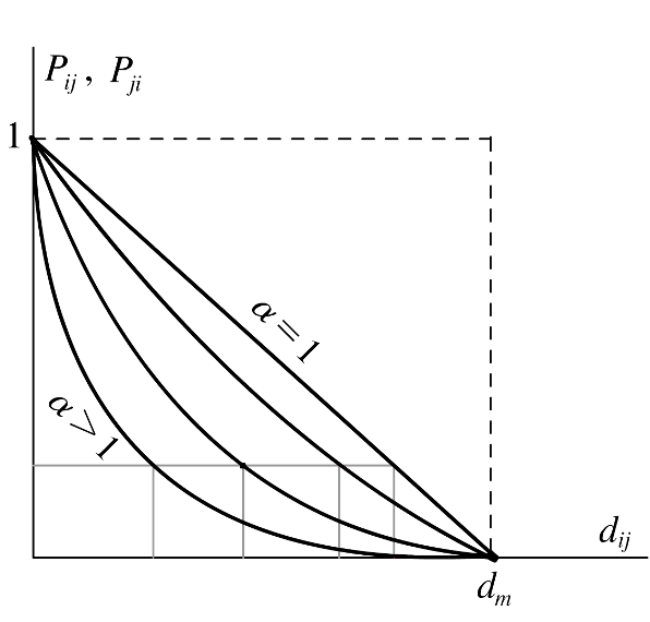
Figure 1. Effect of parameter α 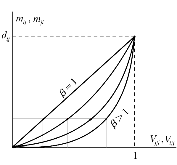
Figure 2. Effect of parameter β - 2.8
- Figure 1 shows how (1) works with increasing values of α . For any values of α and t we have the following properties: Pij → 1 if dij → 0, whereas Pij → 0 if dij → dm, being Pij decreasing and convex in dij. In addition, for higher values of α , affinity has a more local behavior: given a probability Pij, the interaction radius of any agent is [0,R α ], where R α decreases when α grows. Moreover, a small change in distance d changes the probability of interaction Pij more dramatically for smaller values of d.
- 2.9
- In each discrete time period more than one interaction is possible. Using an asynchronous– random updating mechanism (see, for example, Miller & Page 2004) we order all possible pairs (i, j) of agents (nodes in the space of characteristics) randomly, and so the discrete time period is divided into steps where only one potential interaction can be carried out. Then we check if the interaction between them (that happens with probability Pij) really occurs. In this case, an edge is created joining both nodes i and j, which remains until the next potential interaction is checked. In case of no interaction (which happens with probability 1−Pij), no edge between i and j exists until the following updating. Note that each potential edge is updated once per period. The discrete time period then finishes after the n(n−1) steps of potential social interaction and the last n steps of potential innovation by each agent which change the position of the nodes but not the existing connections (the pseudo-code of the model can be found in the appendix).
Intensity of emulation
- 2.10
- Once two agents interact, they approach each other, so that they become more similar (Castellano et al. 2009; Deffuant et al 2000). However, that movement is not symmetrical, but rather the more visible, famous or prestigious agents have greater persuasive power, in line with Corneo and Jeanne (1999) and Deffuant et al (2002).
- 2.11
- In order to formalize this assumption, we define the visibility of a given agent i in t as:
(2) Notice that, Vi(t) ∈ [0,1], with Vi(t) = 0 if the agent i does not interact in t, and Vi(t) = 1 if all interactions in t are made with the agent i. If two given agents i and j interact in t, the relative visibilities of the agent i with respect to j and of the agent j with respect to i are respectively:
(3) These relative visibilities determine the movement (distance covered) of agents i and j at step t, which is produced along the segment (edge) that joins Xi(t) and Xj(t) in the following way:


(4) where mij(t), mji(t) ∈ [0, dij(t)] are given by:
(5) where β ≥ 1 is a parameter, constant for every agent and period, that controls the intensity of the emulation.
- 2.12
- Note that mij(t) + mji(t) ≤ dij(t), and so the distance between agents i and j is always shortened in each step of social interaction, that is: dij(t+1) ≤ dij(t). Note also that, if agent j has a higher relative visibility in t than i (Vj/i(t) > Vi/j(t)), agent i will be more attracted to j than j to i (mij(t) > mji(t)). Moreover, given the nonlinear expressions of mij(t) and mji(t), a higher relative visibility is required when β grows in order to obtain the same relative movement[1] (see Figure 2).
Innovation
- 2.13
- Emulation, in the way that it has been defined, always causes (with more or less probability) agents to approach each other, thus generating dynamics that eventually lead to the long term convergence of all trends into only one (with a convergence speed that depends on the values of parameters α and β ). Therefore, all diversity disappears and one final trend emerges in which all agents are located.
- 2.14
- In order to counterbalance those contraction dynamics, we introduce the possibility that agents can change their social position for reasons beyond social interaction. In this way, the innovation capacity of agents (Said et al. 2002; Witt 2001; Mark 1998), closely related to freedom of choice and thought, also plays an important role in our model. Hence innovation is assumed to be the result of a process of individual exploration, not related to social interaction mechanisms. Specifically, we consider that any agent i, located at position Xi(t) at the end of period t (once the emulation process has finished), can decide to switch, with a certain probability p > 0, to another social position Xi(t+1), given by an n-dimensional random variable with a continuous uniform distribution over the social space S = [0,1]n. In that way the parameter p controls the proportion of agents innovating in each period, that is, the level of innovation of the society.
- 2.15
- Thus the innovation process only updates the position of the nodes that innovate, leaving the structure of the network (edges, that is connections between nodes, only matter in the emulation process) unchanged.
Implementation and results
- 3.1
- The implementation of the computational model is carried out in the following way: for each given combination of parameter values, we generate 50 simulations from random realizations of the initial conditions, discarding the first 4000 iterations (discrete periods) and using[2] the next 2000; the usual cluster analysis is performed to identify the existing trends[3]. For an easier graphical display, a 2-dimensional space of characteristics was considered, even though the results obtained seem to be robust for greater dimensions according to the large number of simulations conducted.
- 3.2
- We carry out two kinds of complementary analyses: one for trends and the other for trend areas. The following properties are of special interest in the analysis of trends:
- Number of representative trends (those that are greater in size than a given threshold, specifically set to 5% of the population).
- Average size of the representative trends.
- Gini coefficient[4] as a measure of the inequality between sizes of trends (all kinds, representative or not). We also include size/rank diagrams to show the unequal distribution of representative trends.
- Dynamism index. We introduce this index to quantify how dynamical the social system is, defined as the average number of changes in the ranking of representative trends within consecutive periods. In particular, we order the representative trends by size in each period and then we calculate the number of changes in position (number of permutations of the ranking) within every two consecutives periods.
- 3.3
- Whereas other partitions (different in number of divisions, size and shape) are possible, we divide each characteristical dimension into 5 parts of equal size[5]. As a result 25 squared areas of trends are obtained, where we study:
- The time evolution of the proportion of agents belonging to each area.
- The weight of each trend area, which represents the probability that any agent is located in a given trend area at any period, is calculated by normalizing the number of agents belonging to that area at any time of any simulation.
- The probability of each trend area becomes dominant, calculated by normalizing the number of times that the given trend area has more agents than any other at any time of any simulation.
- 3.4
- In order to explore the space of parameters values, we consider several scenarios so that only one parameter is explored per scenario, keeping the others constant. The proposed model includes three parameters (α, β and p) and one constant (the size of population N), however the results obtained in the large number of simulations conducted suggest that α and p are the relevant parameters for the dynamics, where β and N have only minor effects, which are basically related to the convergence speed towards the asymptotic state of the system[6]. Thus, we focus our attention only on studying parameters p and α, keeping β = 6 and N = 75 fixed[7].
Scenario 1
- 3.5
- In this scenario, p varies for four given values of α. Specifically, we consider:
- p ∈ [0, 0.02] with steps of 0.001,
- α ∈ {10, 14, 18, 22}.
- 3.6
- The results obtained are shown in Figures 3 and 4. For α ≤ 10 and p∈[0,0.02] the system always exhibits a process of homogenization (with only one representative trend). However for α > 10 a process of diversification (existence of several representative trends) is possible. In particular:
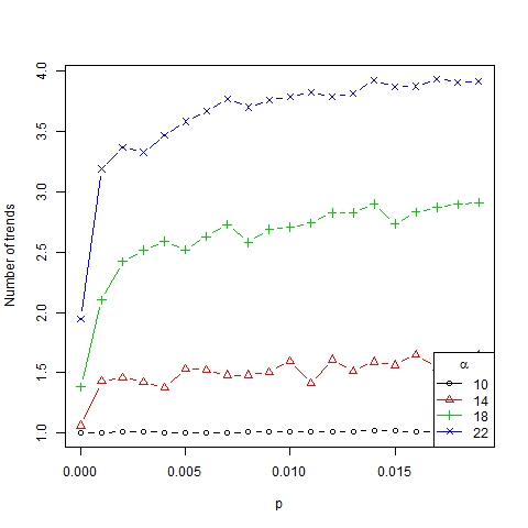
Figure 3. Number of trends as a function of p for β =6, N=75 and different values of α 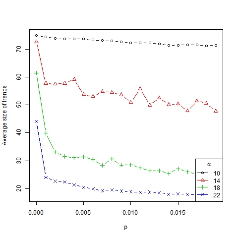
Figure 4. Average size of trends as a function of p for β =6, N=75 and different values of α - If p ≈ 0, a homogenization process of trends toward just one is triggered. So the lack of innovation in society produces a convergence of dynamics towards a stationary point and it leads to only one representative trend in the long term (in line with Malarz et al. 2011).
- If 0 < p < K, a diversity of trends arises. This is similar to the model of Mark (1998), who considered a local convergence of dynamics according to homophily (the parameter α in our model) and the generation of new bits of culture (p > 0 in our case) was enough to produce different subcultures (diversity of trends). In our model, interaction between different trends can be triggered in two ways: when two trends are close and can merge entirely or partially, and when agents change trends due to innovation.
- If p > K (p is large enough[8]), one trend per agent is obtained, implying all members of society become isolated. Note that too much innovation leads to completely erratic (random) dynamics.
- 3.7
- Thus we have established that the role of parameter p in the number, size and dispersion of trends is mainly qualitative, no matter which value we have, as long as it is positive (see Figure 5) and not too large. Furthermore the dynamism index (which measures the average number of changes in the ranking of representative trends for two consecutive periods of time) depends on p linearly (see Figure 6). In this way, the higher the innovation, the more dynamical and changeable the society becomes.
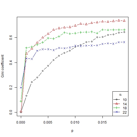
Figure 5. Gini coefficient as a function of p for β =6, N=75 and different values of α 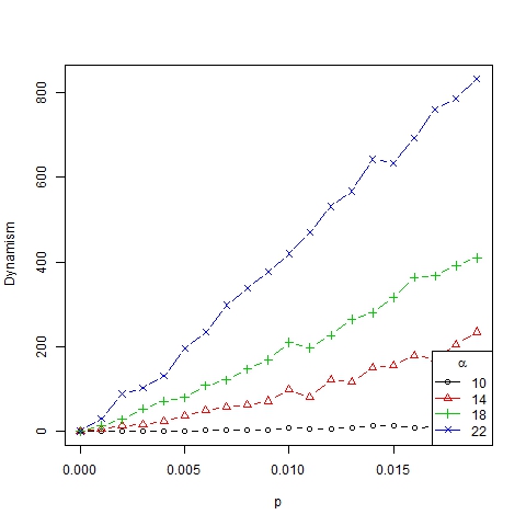
Figure 6. Dynamism index as a function of p for β =6, N=75 and different values of α - 3.8
- Finally we show the unequal distribution of trend sizes in Figures 7 and 8 (in this case, with a log-log scale) by means of size/rank diagrams, representing the average size of clusters in the first to sixth position in the ranking of representative trends.
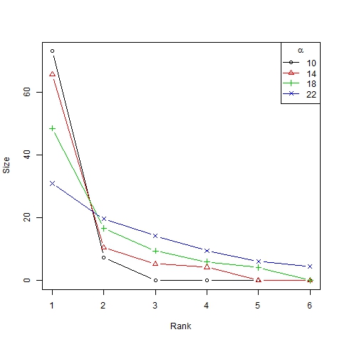
Figure 7. Size/rank diagram for β =6, N=75 and different values of α 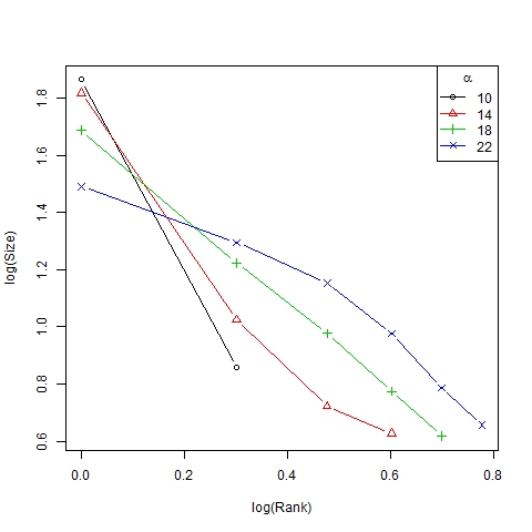
Figure 8. Log-log size/rank diagram for β =6, N=75 and different values of α Scenario 2
- 3.9
- In this scenario, α varies for four given values of p. Specifically, we consider:
- p ∈ {0.002, 0.003, 0.004, 0.005},
- α ∈ [10, 30] with steps of 2.
- 3.10
- The results obtained are shown in Figures 9, 10, 11 and 12. Note that the number of emerging trends depends mainly on parameter α (Figure 9). Thus, with α = 18 two or three representative trends are usually generated in society[9], while at the same time some other minor trends co-exist (as can be deduced from the high Gini coefficient, see Figure 11).
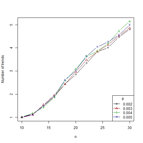
Figure 9. Number of trends as a function of α for β =6, N=75 and different values of p 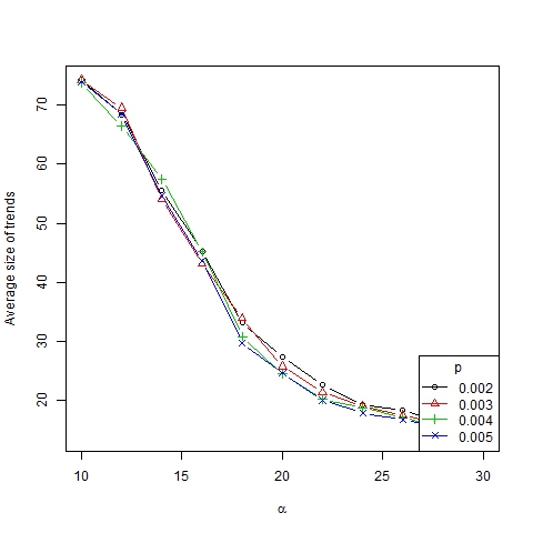
Figure 10. Average size of trends as a function of α for β =6, N=75 and different values of p 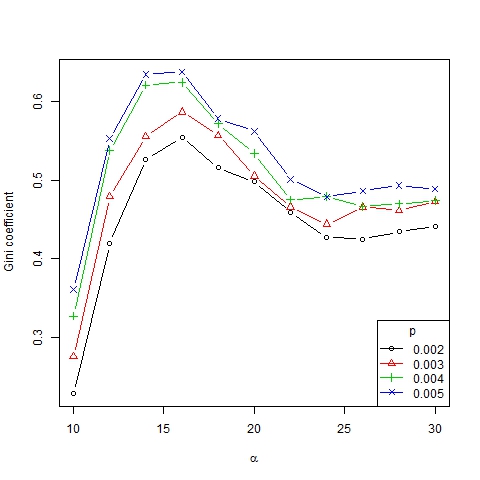
Figure 11. Gini coefficient as a function of α for β =6, N=75 and different values of p 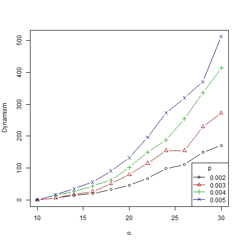
Figure 12. Dynamism index as a function of α for β =6, N=75 and different values of p - 3.11
- The number of trends as a function of α seems to adjust to an S-shaped curve, whereas the average size of trends seems to adjust to a decreasing S-shaped curve (Figure 10). The number of trends in the asymptotic state of the system gives us information about the degree of diversity of a society. According to this measurement we can identify three different convergence types:
- If α < 14, all the agents converge to the same trend, that is, only one trend is present. Following Gargiulo and Mazzoni (2008), we call this a uniformity regime. This regime is relatively independent of the value of the other parameters.
- If 14 < α < 18, a great many trends arise even though only a few of them (usually two or three) are representative (which is implied by the high Gini coefficient for these values of α). It is a transition phase that corresponds with the strong majority regime of Gargiulo and Mazzoni (2008).
- If α > 18, many different trends with similar size remain for the long term. We call it a diversity regime (regime of pluralism in words of Gargiulo and Mazzoni, 2008). It is also consistent with Axelrod (1997) where it was found that "local convergence can lead to global polarization" and stable minority subcultures can persist because of the protection of structural holes created by cultural differences that preclude interaction, thereby insulating agents from homogenizing tendencies.
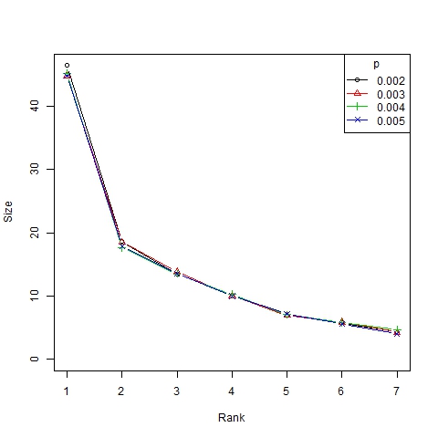
Figure 13. Size/rank diagram for β =6, N=75 and different values of p 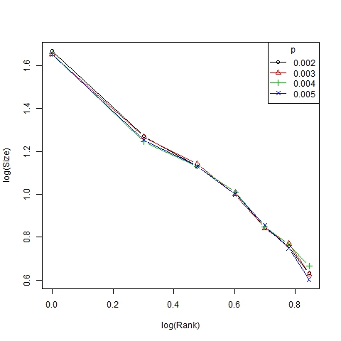
Figure 14. Log-log size/rank diagram for β =6, N=75 and different values of p - 3.12
- Finally, note that the dynamism index depends on α in a nonlinear manner (Figure 12). Roughly speaking, we can state that α is the parameter that best explains the dynamics of the system, which is in accordance with the results of Gargiulo and Mazzoni (2008). This can also be figured out from the size/ranks diagrams shown in Figure 13 and, with a log-log scale, in Figure 14. As can be seen, there is no significant difference between the distributions of trend size for different values of p.
Empirical evidence
- 3.13
- The dynamical results of the model seem to be consistent with empirical evidence, as we show using real-world data from the 2007 Andalusia Social Survey, a study based on a random sample of 1850 personal interviews intended to produce comparative data of Andalusia's social reality, and conducted by the Statistical Institute of Andalusia, agency of the Regional Ministry of Economy, Innovation and Science.
- 3.14
- Two specific questions (representing characteristics of our model) were chosen from the survey, each one measured in an eleven-point Lickert-type scale:
Characteristic 1. Feeling about Europe (0 = not European; 10 = strongly European).
Charasteristic 2. Feeling about Ecology (0 = not ecologist; 10 = strongly ecologist). - 3.15
- We apply the same cluster analysis on the empirical data as in the implementation of our theoretical approach, computing the same statistical indicators and estimating the values of α and p that produce similar results[10] (we again consider β = 6 and normalize population size to N = 75).
Table 1: Empirical trends in terms of the level of education
Level of educationNumber of trends Average size Gini coefficient α p Primary 6 11 0.484 34 0.003 Secondary 4 16 0.600 24 0.008 University 2 29 0.639 17 0.012 - 3.16
- As can be seen in Table 1, where all this information is gathered, the estimated values of α and p faithfully reproduce the number and size (out of 75) of social trends existing in analyzed data for different levels of education, as well as the inequality of trend sizes measured by the Gini coefficient. These estimated values are consistent with sociological explanations: better-educated individuals are supposed to be more open-minded, tolerant and thus they are more likely to interact in a more global way (that is, they have lower values of α ), showing at the same time a higher willingness of innovation (greater values of p).
- 3.17
- Similar conclusions can be arrived at looking at Table 2, where characteristics were studied in terms of the place of residence. Again the estimated values of α and p match the number, size and inequality of social trends closely (except for the Gini coefficient obtained for Town), which is consistent with sociological explanations: individuals living in more cosmopolitan areas are supposed to be more open, tolerant, with easier access to global social networks (lower values of α) and more likely to innovate (greater values of p).
Table 2: Empirical trends in terms of the place of residence
Place of residenceNumber of trends Average size Gini coefficient α p Village (<10000) 6 11 0.481 34 0.003 Town (>10000) 5 13 0.451 30 0.006 Capital of province 4 16 0.600 24 0.008 Analysis of trend areas
- 3.18
- As previously mentioned, each characteristical dimension (x1 and x2) is divided into 5 parts of equal size, which results in a total of 25 square trend areas. We employ matrix notation to denote them: in this way, area i_j is that located on section i of x1 and section j of x2. We select a set of parameters that generates interesting dynamical properties in the evolution of trend areas, in particular, we set the following values (explored in scenario 2 of the trend analysis): α = 24, β = 6, p = 0.003 and N = 75.
- 3.19
- Time evolution of representative trend areas (with a minimum size of 5% of agents) for a specific simulation is shown in Figure 15, showing different phenomena than what are present in the real world, such as fashion or public opinion tendencies: cyclical behavior in trend areas, changes in leadership, extinction and resurgence of trend areas and the struggle between areas which are almost always adjacent. All the areas show cyclical evolutions, but mainly areas 1_1 and 5_2. Areas 5_2 and 2_4 struggle with each other for leadership. Area 5_4 stays latent almost all the time, reactivating from time to time. Area 5_5 oscillates, it begins in the third position, then becomes extinct and eventually reappears. In the end, a struggle between two adjacent areas can be seen (area 5_4 makes 5_5 disappear).
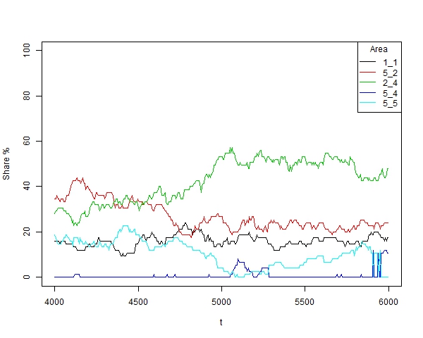
Figure 15. Time evolution of trend areas for a specific simulation with α =24, β =6, p=0.003 and N=75 - 3.20
- Figures 16 and 17 show each trend area's weight and the dominant area's weight, respectively (where darker represents higher weight). The weight of a trend area is defined as the relative number of agents located on that area at any time of any of the 1000 simulations conducted, and represents the probability of any agent belonging to that area in any period. The weight of each dominant trend area is defined by the proportion of times that a given area is dominant at any time of any simulation.
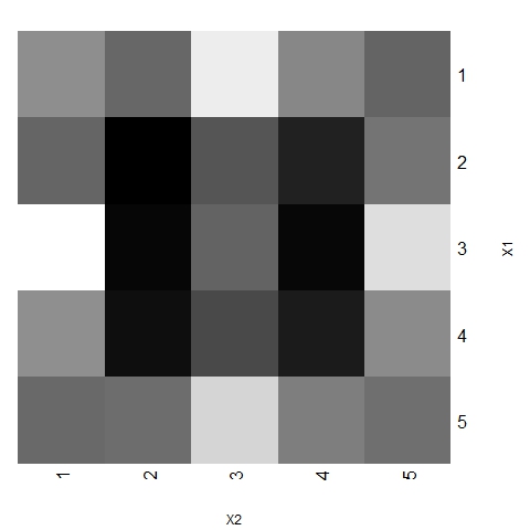
Figure 16. Weight of trend areas for 1000 simulations with α =24, β =6, p=0.003 and N=75 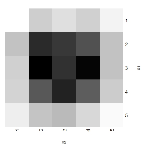
Figure 17. Weight of dominant trend areas for 1000 simulations with α =24, β =6, p=0.003 and N=75 - 3.21
- Figures 16 and 17 show that all areas do not have the same weight. Although a kind of symmetry is present in the system (both characteristical dimensions are treated equally in the theoretical model, not existing preferences for a specific direction), central areas are more likely to have representative trends. In particular, the dominant trend is often located around the central zone, which is consistent with the evidence in many social processes.
- 3.22
- In order to further explore the trend areas we order them according to their distance[11] from the central zone 3_3. Thus we have trend areas at distance 0, 1, sqrt(2), 2, sqrt(5) and sqrt(8). Figures 18 and 19 show the probability for a representative trend, and for the dominant trend respectively, to be located in an area at distance r. Despite representative trends being often found in extreme areas, dominant trends are significantly more likely to be located in central areas (with a probability greater than 0.85 for r ≤ sqrt(2)).
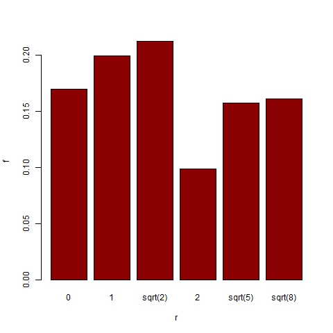
Figure 18. Distribution of trend area location for 1000 simulations with α =24, β =6, p=0.003 and N=75 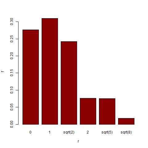
Figure 19. Distribution of dominant trend area location for 1000 simulations with α =24, β =6, p=0.003 and N=75 - 3.23
- The effect of changes in the values of p and α on the position of trend areas is analyzed by means of box-and-whisker diagrams. Figures 20 and 21 show the boxes with quartiles Q1, Q2 (median) and Q3 for the distribution of trend area location, and dominant trend area location respectively, for three different values of p (0.002, 0.003 and 0.004). Figures 22 and 23 show the corresponding box-and-whiskers diagrams for three values of α (18, 24 and 30). As expected, p has a minor effect on trend area location. However α does play an important role in the process: both representative and dominant trend areas move away from the center relatively when α increases.
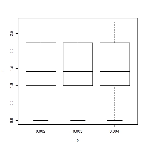
Figure 20. Box-plot of trend area location for α =24, β =6, N=75 and different values of p 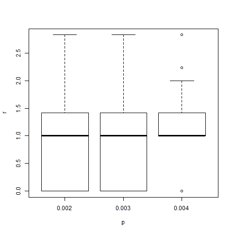
Figure 21. Box-plot of dominant trend area location for α =24, β =6, N=75 and different values of p 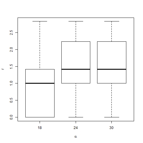
Figure 22. Box-plot of trend area location for β =6, p=0.003, N=75 and different values of α 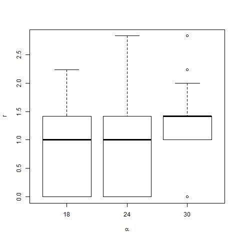
Figure 23. Box-plot of dominant trend area location for β =6, p=0.003, N=75 and different values of α
Conclusion
- 4.1
- In this paper we introduce a descriptive computational model that reproduces the mechanism of underlying social processes led by emulation. With a few assumptions this model can respond to some questions of interest, such as how and why highly skewed distributions emerge in human societies, where few trends are representative and co-exist with several minor trends.
- 4.2
- The model offers several results, some of which are intuitive whereas others are somewhat unexpected. One of the latter type is that if a society is too tolerant and permeable (α < 14), all the agents converge to only one trend that leads to uniformity; all initial diversity in society disappears. Moreover if society's tolerance is moderate, many trends arise but with a high dispersion of size, only a few of them being truly representative. Finally, in highly intolerant societies a considerable degree of segregation is reached, where lots of trends arise with a similar size. This effect can be seen, for example, in web communities, in communities of minority religions or in associations devoted to some sports. These communities are characterized by members that have similar opinions, beliefs or tastes, but differ from what is average in the society (see Schelling 1969 or Stauffer and Solomon 2007). In the context of public opinion, homophily, as evidenced by a higher propensity of agents to interact with those more similar, is the mechanism that leads individuals to cluster in communities (Kandel 1978; Mcpherson et al. 2001; Galam 2005; Centola et al. 2007).
- 4.3
- Additionally, as expected, the more innovative the society is (higher p), the more dynamic it becomes. In other words, a larger number of changes are made in the ranking of trends, although this does not affect the distribution of trend size. That is, when the degree of innovation is increased, trends more often decrease in size, which leads to changing the order more frequently (it might even happen that the dominant trend goes down and never comes back to be the leader), whereas the relative weight of trends sorted from larger to smaller remains invariant.
- 4.4
- Finally, we established that a high level of innovation in a society is not necessary in order to reach pluralism, but just a little is enough (p > 0). In fact, too much innovation (p large enough) might be damaging by leading agents to isolation.
- 4.5
- The proposed model can reproduce several real phenomena in social processes which emulation is present, such as fashion or public opinion tendencies: cyclic evolution in trend areas, changes in leadership, extinction and resurgence of trend areas and the struggle between close areas.
- 4.6
- Note that not all areas have the same weight. The dominant trend is usually located in the central zone, although real cases exist where extremes becomes a majority. As Deffuant et al. (2002) state, Germany in the 30's is a dramatic example. However, the evidence shows that dominant positions are usually moderate, which is consistent with the results obtained.
Appendix: Pseudo-code of the model
-
- Create a graph in the space of characteristics with a fixed set of N nodes, initially without edges. The initial position of each node is randomly drawn from a uniform distribution.
- For each period:
2.1. Randomly sort a list of all possible edges and then check them.
2.2. For each edge (i, j):
2.2.1. Delete the edge (i, j) from the graph if it exists.
2.2.2. With probability pij the agents i and j interact (see: Affinity).
2.2.2.1. They approach each other (see: Intensity of emulation).
2.2.2.2. The edge (i, j) is added to the graph.
2.3. Randomly sort the list of nodes.
2.4. For each node i:
2.4.1. With probability p the node updates its position drawn from a uniform distribution (see: Innovation).
Notes
-
1 The assumption β ≥ 1 implies that functions mij and mji are increasing and convex in Vj/i and Vi/j respectively.
2 Thus we remove the transition to the asymptotic state of the system. Standard deviation (in t) is used to check if the number of iterations is enough to keep emergent properties stable.
3 We use an agglomerative hierarchical clustering algorithm with average linkage criterion and Euclidean distance, cutting the dendogram at a level of similarity fixed on 0.1.
4 Gini coefficient is a measure of statistical dispersion, commonly used as a measure of inequality of income or wealth. A Gini coefficient of 0 expresses perfect equality whereas a Gini coefficient of 1 expresses maximal inequality among values (for example, where only one individual has all the income).
5 In a similar way to a five-point Likert-type scale, commonly used in research that employs questionnaires with the typical format: strongly disagree, disagree, neither agree nor disagree, agree, strongly agree.
6 According to our simulations, fixed α and p, the number and size of trends remain fairly stable for values of β between 4 and 15, although the time required to reach the asymptotic state significantly increases with β . Similar comments can be made about N∈[50,180].
7 The ranges of values for α and p were chosen so that all possible regimes were obtained (only one representative trend, a few of them or a state with a great polarization of trends).
8 The steady increase in the number of trends (when p increases) eventually leads to the complete polarization of society. The specific value of K that produces this situation depends on α (lower values of K for greater values of α ).
9 It reminds us of the two- or three-party systems common in many modern democracies.
10 We consider the asymptotic state of our model in order to estimate the parameters from the survey. Thus we assume that the two specific questions considered have been widely discussed and therefore public opinion on these issues is sufficiently consolidated. Note that even after the asymptotic state is reached, social trends could change into the future as happens in our model where the representative trends and their weights change over time.
11 Euclidean distance from the middle of each squared area to the middle of the central square 3_3. Sqrt denotes the square root.
References
-
ARTHUR W. B. (1994). Inductive Reasoning and Bounded Rationality. The American Economic Review, 84(2), 4067–411.
AXELROD, R. (1997). The Complexity of Cooperation. Princeton University Press.
BATTAGLINI, M. (2005). Sequential voting with abstention. Game Econ. Behav., 51(2), 445–463. [doi:10.1016/j.geb.2004.06.007]
CASTELLANO, C., Fortunato, S. & Loreto, V. (2009). Statistical physics of social dynamics. Reviews of modern physics, 81(2), 591–646. [doi:10.1103/RevModPhys.81.591]
CENTOLA, D., Gonzá lez-Avella, J. C., Eguiliz, V. M. & San Miguel, M. (2007). Homophily, Cultural Drift, and the Co-Evolution of Cultural Groups. Journal of Conflict Resolution, 51(6), 905–929. [doi:10.1177/0022002707307632]
CHEN, Y. F. (2008). Herd behavior in purchasing books online. Comput. Hum. Behav., 24(5), 1977–1992. [doi:10.1016/j.chb.2007.08.004]
CHRISTAKIS, N. A. & Fowler, J. H. (2007). The spread of the obesity in a large social network over 32 years. N. Engl. J. Med., 357(4), 370–379. [doi:10.1056/NEJMsa066082]
CORNEO, G. & Jeanne, O. (1999). Segmented communication and fashionable behavior. Journal of economic behavior and organization, 39(4), 371–385. [doi:10.1016/S0167-2681(99)00046-3]
COWAN, R., Cowan, W. a& Swann, P. (1997). A model of demand with interactions among consumers. International Journal of Industrial Organization, 15(6), 711-732. [doi:10.1016/S0167-7187(97)00008-8]
CUCKER, F., Smale, S. & Zhou, D. X. (2004). Modeling Language Evolution. Foundations of Comput. Math., 4(3), 315–343. [doi:10.1007/s10208-003-0101-2]
DEFFUANT, G., Neau, D., Amblard, F. & Weisbuch, G. (2000). Mixing beliefs among interacting agents. Advances in Complex Systems, 3(01/04), 87–98. [doi:10.1142/S0219525900000078]
DEFFUANT, G., Amblard, F., Weisbuch, G. & Faure, T. (2002). How can extremism prevail? A study based on the relative agreement interaction model. Journal of Artificial Societies and Social Simulation, 5(4) 1 https://www.jasss.org/5/4/1.html.
DÖRNER, D. (1999). Bauplan für eine Seele. Rowohlt, Hamburg.
DYER, J. R. G., Ioannou, C. C., Morrell, L. J., Croft, D. P., Couzin, I. D., Waters, D. A. & Krause, J. (2008). Consensus decision making in human crowds. Anim. Behav., 75(2), 461–470. [doi:10.1016/j.anbehav.2007.05.010]
GALAM, S. (1997). Rational Group Decision Making: a random field Ising model at t = 0. Physica A, 238(1), 66–80. [doi:10.1016/S0378-4371(96)00456-6]
GALAM, S. (2005). Heterogeneous beliefs, segregation, and extremism in the making of public opinions. Physical Review E., 71(4), 461–423. [doi:10.1103/PhysRevE.71.046123]
GARGIULO, F. & Mazzoni, A. (2008). Can Extremism Guarantee Pluralism?. Journal of Artificial Societies and Social Simulation, 11(4) 9 https://www.jasss.org/11/4/9.html.
KANDEL, D. B. (1978). Homophily, Selection, and Socialization in Adolescent Friendships. American Journal of Sociology, 84, 427–436. [doi:10.1086/226792]
KENRICK, D. T., Maner, J. K., Butner, J., Li, N. P., Becker, D. V. & Schaller, M. (2002). Dynamical evolutionary psichology: Mapping the domains of the new interactionist paradigm. Pers. Soc. Psychol. Rev., 6(4), 347–356. [doi:10.1207/S15327957PSPR0604_09]
KULAKOWSKI, K. (2009). Opinion polarization in the Receipt-Accept-Sample model. Physica A., 388(4), 469–476. [doi:10.1016/j.physa.2008.10.037]
KUMAR, M. (2007). A Journey into the Bleeding City: Following the Fooprints of the Rubble of Riot and Violence of Eathquake in Guarat, India. Psychol. Dev. Soc., 19(1), 1–36. [doi:10.1177/097133360701900101]
LATANÉ, B. & Nowak, A. (1997). Self-Organizing Social Systems: Necessary and Sufficient Conditions for the Emergence of Clustering, Consolidation, and Continuing Diversity. In: G.A. Barnett and F.J. Boster (eds.), Progress in Communication Sciences. Ablex Publishing Corporation, 1–24.
LIVIATAN, I., Trope, Y. & Liberman, N. (2008). Interpersonal similarity as a social distance dimension: Implications for perception of others' actions. Journal of experimental social psychology, 44(5), 1256–1269. [doi:10.1016/j.jesp.2008.04.007]
MALARZ, K., Gronek, P. & Kulakowski, K. (2011). Zaller-Deffuant Model of Mass Opinion. Journal of Artificial Societies and Social Simulation, 14(1) 2 https://www.jasss.org/14/1/2.html.
MARK, N. (1998). Beyond individual differences: social differentiation from first principles. Am. Sociol. Rev., 63(3), 309–330. [doi:10.2307/2657552]
MCPHERSON, M., Smith-Lovin, L. & Cook, J. M. (2001). Birds of a Feather: Homophily in Social Networks. Annual Review of Sociology, 27, 415–444. [doi:10.1146/annurev.soc.27.1.415]
MILLER, J. H., & Page, S. E. (2004). The standing ovation problem. Complexity, 9(5), 8–16. [doi:10.1002/cplx.20033]
ORLEAN, A. (1995). Bayesian Interactions and Collective Dynamics of Opinions: Herd Behavior and Mimetic Contagion. Journal of Economic Behavior and Organization, 28(2), 257–274. [doi:10.1016/0167-2681(95)00035-6]
RANDOW, G. (2003). When the centre becomes radical. Journal of Artificial Societies and Social Simulation, 6(1) 5 https://www.jasss.org/6/1/5.html.
SAID, L. B., Bouron, T. & Drogoul, A. (2002). Agent-Based Interaction Analysis of Consumer Behavior. AAMAS 2002, Bologna, Italy. [doi:10.1145/544741.544787]
SALGANIK, M. J., Dodds, P. S., & Watts, D. J. (2006). Experimental study of inequality and umpredictability in an artificial cultural market. Science, 311(5762), 854–856. [doi:10.1126/science.1121066]
SCHELLING, T. C. (1969). Models of Segregation. The American Economic Review, 59(2), 488–493.
SCHOR, J. (1999). The Overspent American. Harper Perennial, New York.
SHILLER, R. J. (2000). Irrational exuberance. Princeton University Press.
SHILLER, R. J. (2002). Bubbles, human judgment, and expert opinion. Fin. Analysts J., 58(3), 18–26. [doi:10.2469/faj.v58.n3.2535]
SORNETTE, D., Woodard, R. & Zhou, W. X. (2009). The 2006–2008 oil bubble: Evidence of speculation, and prediction. Physica A. – Stat. Mech. Applic., 338(8), 1571–1576. [doi:10.1016/j.physa.2009.01.011]
STAUFFER, D. & Solomon, S. (2007). Ising, Schelling and self-organising segregation. European Physical Journal B-Condensed Matter and Complex Systems, 57(4), 473–479. [doi:10.1140/epjb/e2007-00181-8]
WEISBUCH, G. & Boudjema, G. (1999). Dynamical aspects in the Adoption of Agri-Environmental Measures. Adv. Complex Systems, 2(1), 11–36. [doi:10.1142/S0219525999000035]
WITT, U. (ed.), (2001). Escaping satiation. The demand side of economic growth. Springer-Verlag.