
 Abstract
- In this study, we are interested in the problem of determining the pricing and timing strategies of a new product by developing an agent-based product diffusion simulation. In the proposed simulation model, agents imitate behavioural consumers, who are reference dependent and risk averse in the evaluation of new products and whose interactions create word-of-mouth regarding new products. Pricing and timing strategies involve the timing of a new product release, the timing of providing a discount on a new product, and the relative rates of discounts. We conduct two experiments in this study. In both experiments, we consider the urban young person segment in the mobile phone market in Korea, in which three major new products - two smartphones and one convergence product - compete with one another. The first experiment is sensitivity analysis on the product life cycle and social influence. The objective is to observe how consumer agents behave as the product life cycle and the degree of sensitivity on social influence change. The second experiment is sensitivity analysis on time-to-market, time-to-discount, and amount-to-discount. The marketing strategy that maximises the sales volume (or revenue) of the new convergence product is sought from the sensitivity analysis. Based on the result, we provide pricing and timing implications for firms pursuing sales volumes (or revenue) increase.
- Keywords:
- Product Diffusion, Pricing and Time Strategies, Korean Mobile Phone Market, Sensitivity Analysis
Introduction
- 1.1
- In recent years, a technological gap among global manufacturing firms has narrowed, causing product marketing to be emphasised more than ever. Firms typically face three fundamental questions related to the release and pricing of a new product: the release time of a new product (i.e., time-to-market), the discount time of the product (i.e., time-to-discount), and the discount rate (i.e., amount-to-discount). To provide the best solutions to the three issues, it is essential to understand how individuals attach value to the new product. Here, the value (or utility) of a product is a measure of the satisfaction from the consumption of the product. In this paper, as a support tool to address these issues, we propose a social simulation that focuses on consumers' psychological bias and social interaction in the evaluation of competing products.
- 1.2
- Over the last two decades, psychological bias has been recognised as an important factor in modelling people's economic behaviours. In particular, when consumers choose products, most tend to be reference dependent and risk averse. For example, consumers are accustomed to evaluating the value of a new product by comparing it to their products in use as references. In addition, most consumers sense a wider gap when the value gained from the product in use is larger than the value expected from the new product than when the value gained is less than the value expected; even when their absolute difference is the same. That is, people have a loss aversion tendency that places more emphasis on losses than on gains.
- 1.3
- The advance of information technology creates social network services, which people, especially young individuals, use to share information of interest and sometimes to make decisions, such as product choice, based on shared information. The word-of-mouth (WOM) on product performance created by consumers in a social network has increasingly affected the success of new products (Kempe et al. 2003; Godes & Mayzlin 2004). Unfortunately, modelling the principle of network-wide WOM generation in a monolithic way is very difficult because consumers in the social network are influenced by and influence different people at different times. For a product attribute that consumers are sensitive to, such as price, a change affects their product choices. However, the time when the wave of WOM on the price change reaches individual consumers and the degree to which WOM impacts their product choices are not directly measurable.
- 1.4
- A multi-agent simulation model is known as a good instrument for modelling the social interactions of actors. The social simulation model proposed in this paper is a multi-agent simulation in which agents represent consumers. In the model, we design behavioural consumer agents who are reference dependent and risk averse. For modelling behavioural consumer agents, we adopt prospect theory (Kahneman & Tversky 1979), which describes people's psychological biases when they engage in economic behaviours. And, the theory is known as more descriptive and realistic rather than the other choice models which are known as normative (Bleichrodt et al. 2001). The other choice models such as expected utility theory (EUT) (Harrison & Rutström 2009) and technology acceptance model (TAM) (Davis 1986) are only focused on rational and reasonable process in decision-making. As stated by Davis et al. (1989), TAM utilises theory of reasoned action (TRA) (Fishbein & Ajzen 1975) as a theoretical foundation for identifying the causal relationships between perceived usefulness and perceived ease of use, and users' attitudes, intentions and actual computer adoption behaviour. This is designed to apply TRA only to computer usage behaviour.
- 1.5
- We also incorporate the social interaction of behavioural consumer agents in the model so that collective opinions on competing products formed by WOM affect product choices of potential adopters. Representing the output of the model are predicted sales-volume trajectories of competing products. By simulating product diffusion with possible pricing and timing combinations, we are able to determine the strategy that maximises the chances of a new product's success in a target market.
- 1.6
- As a case study, we consider the Korean smartphone market. Like any other electronic gadgets, a new smartphone is often compared to the phone in use by a consumer. The smartphone market is becoming more competitive because not only products in the same product family but also convergence products, which overlap more than one different product family, are being developed and released into the market by high-technology firms. For example, smartphone and tablet PCs (personal computer) are converging into a new convergence product. For our case study, we have sampled Korean young people from smartphone users. In the case of Korea, the market share of smartphones in the phone market is increasing rapidly, and one fourth of phone users have smartphones. Among the users, the most critical segment is thought to be urban young people, who are often known to be sensitive to the pricing of high-tech products and the timing of their release because they have small budgets and a desire to obtain new high-tech products.
- 1.7
- Our study provides three main contributions. First, we formulate a behavioural consumer who has reference dependence and risk aversion and the interaction of behavioural consumers within a social network. Second, we simulate the expected sales volumes of a new convergence product and the other competing products in the young people segment of the Korean smartphone market and determine the time-to-market, time-to-discount, and amount-to-discount that maximise the sales volume. Third, we investigate another market situation in which a producer offers two smartphones of different types: a typical phone and a new convergence phone. The use of more than one product release is commonly used in competitive markets to reduce the risk of product failure. However, a product-line problem, the cannibalisation effect, is more pronounced. The cannibalisation effect is the effect of a sales volume decrease in the typical product due to the introduction of the new product similar to the typical product. Under this scenario, we find marketing strategies that provide the minimum and maximum revenues for the producer.
- 1.8
- The remainder of this paper is organised as follows. Section 2 explains relevant agent-based product diffusion models for pricing and timing. Section 3 introduces the details of a proposed behavioural agent simulation model. Section 4 presents experiments and results with pricing and timing implications. Finally, section 5 provides concluding remarks.
Related Work
- 2.1
- Classical economists have considered that a consumer chooses a product with maximum utility. However, empirical studies have found counterexamples against utility maximisation (Camerer & Thaler 1995; Camerer 2008). In many cases, a consumer is likely to rely on simple heuristics, which leads to a satisfactory solution but not the optimal solution with maximum utility. An example is the anchoring effect (Tversky & Kahneman 1974), which explains that a consumer is biased towards the number originally given in the beginning of evaluation. Tversky and Kahneman (1974) once asked subjects to estimate the percentage of African countries in the United Nations after giving them a number between 1 and 100 by a spin of a wheel. Even if the number from a spin of a wheel was irrelevant to the percentage of African countries in United Nations, the subjects overweighed the irrelevant number in estimating the percentage. This phenomenon is widely observed in laboratory experiments (Chapman & Johnson 2002) and in real economic contexts as well, such as the housing market (Genesove & Mayer 2001), the stock market (Barberis et al. 2001), and art auctions (Beggs & Graddy 2009). A consumer under uncertain conditions (i.e., relatively unaware of a new product) estimates a new product by setting a reference point (i.e., anchoring point) and by calculating the difference of the new product from the reference. Another example is loss aversion (Kahneman & Tversky 1979), where a consumer is relatively more sensitive to the possibility of losing property or money than to that of gaining the same amount of property or money, a phenomenon recently investigated with a biological experiment (Tom et al. 2007). The prospect theory proposed by Kahneman and Tversky (1979) generalised the anchoring effect (i.e., reference dependence) and loss aversion in human decision making. Because decision making involves several criteria or attributes, Tversky and Kahneman (1991) extended the original prospect theory to multi-attribute prospect theory. Hardie et al. (1993) applied multi-attribute prospect theory to the product choice of a single consumer without the consideration of social interaction. Other recent applications of prospect theory include route choice modelling (Xu et al. 2011), resource allocation (Bromiley 2009), and portfolio choice (He & Zhou 2011).
- 2.2
- Multi-agent modelling and simulation is a computational tool used at the micro level. It imitates a natural market dynamic by specifying individual product adoption processes and implementing WOM, which is again fed back to the individual decision making of potential consumers. Due to its modelling power, multi-agent simulation has received much attention from researchers who investigate collective market dynamics (Janssen & Jager 2003; Delre et al. 2007a; Kim et al. 2011; Lee et al. 2013). However, these studies do not concern marketing strategies, such as the timing and pricing of a new product. Because the predictive power of traditional mathematical diffusion models (e.g., the general linear model (Mardia et al. 1979), and the growth model (Bass 1969; Mahajan et al. 1990)) is suspected to be low in dynamic and volatile markets (Jager 2007; Zenobia et al. 2009; Orrell & McSharry 2009), studies of marketing strategies based on multi-agent simulation are emerging. Not only the timing of promotion strategies, such as mass media campaigns and mass communication activities, but also the pricing relevant to promotion strategies (e.g., informing consumers a price-cut) of a new product represent the main issue (Delre et al. 2007b; Diao et al. 2011; Gunther et al. 2011). Delre et al. (2007b) have noted consumers' preferences, needs, and social factors as being determinants of the success of marketing strategies in a fashionable market. However, those studies have not considered psychological biases (reference dependence and loss aversion) that influence the determinants. Furthermore, none has combined the release time of a new product with the timing of promotions and pricing. In this paper, we introduce the concept of providing the right discount rate at the right time with respect to the release time of a new product.
Behavioural consumer agent model
-
Simulation overview
- 3.1
- The proposed model simulates product choice processes of consumers in a market. In the model, each consumer agent imitates a consumer's product choice process, and the connection structure of consumer agents corresponds to consumers' social network through which they exchange product information. We assume that the social network of consumers in a market is a form of a small world network (Watts & Strogatz 1998) adopted in recent product diffusion studies (Janssen & Jager 2003; Kim et al. 2011; Lee et al. 2013). The small-world network is a variation of a regular network that is a normal lattice where every node (e.g., consumer) is linked to its neighbours with a fixed degree of connectivity. The small-world network emerges as the result of randomly rewiring a fraction of the links of every node. The fraction of links is called the rewiring probability. In the small-world network, it is possible to connect any two nodes through only a few links.
- 3.2
- The simulation considers a market situation in which multiple new products compete with each other. The model allows competing products to be launched in the market at different times, providing an environment for firms to investigate the release timing effect on total sales volume. We assume that new products and products in use of consumer agents have multiple attributes, but these attributes may not be identical. If a product does not have a certain attribute, e.g., the second-generation mobile phone has no wireless Internet feature, the attribute value of the product endowed by consumer agents is set to zero. Here, the attribute value does not mean physical value but a satisfaction degree of a consumer from the use of the attribute. In our model, we assume that consumer agents endow values in a bounded interval including zero for each attribute. If some consumers do not have products in use comparable to new products, all attribute values of the products in use are set to zero.
- 3.3
- During a simulation run, consumer agents continue to update attribute values of new products with the consideration of psychological biases (i.e., loss aversion and reference dependence) and social influence. The simulation allows a firm to change the attribute values of its new product in the middle of the simulation run, such as a price discount set at a certain time, and to observe the effect of the change on the sales volume. Almost every consumer agent (though surely not all) decides to choose one of some products at the moment when the values of the products become higher than the value of product in use. This purchase timing makes it possible for some consumer agents not to buy new ones if the values of products in use remain higher than those of all new products until the end of the simulation run. We assume that the value of the product in use decays over time. If the decay speed is fast, as is the case of fashionable products with short life cycles (e.g., mobile phones and gaming devices), few consumer agents complete the simulation without making a purchase.
Initialisation
- 3.4
- The proposed simulation model runs through an initialisation stage and an execution stage. In the initialisation stage, consumer agents are connected such that their interaction structure has a form of a small world network. In our experiment, we set the degree of connectivity as 4 and the rewiring probability as 0.05 as the optimal social network for Korean netbook market found in Lee et al. (2013). Next, every agent is assigned four personal characteristics: initial attribute values for new products, attribute values for the product in use, product attribute weights, and the degree of sensitivity to social influence. In the beginning of the simulation, they initially obtain uncertain information on new product attributes; they assess attribute values of new products by referring to attribute values of products in use (i.e., reference dependence); they weigh product attributes uniquely; they reflect the social influence of neighbours at different degrees when they are undergoing the product evaluation process. Empirical probability distributions are built for the four characteristics through a questionnaire, and consumer agents are assigned individual values randomly using the distributions. In addition, to let consumer agents be loss averse, every agent requires a degree of loss aversion. We assume that each consumer agent has a different degree of loss aversion for each product attribute, which is equal to the consumer agent's weight on the product attribute. That is, a consumer is more loss averse to an attribute that is believed to be more important.
Execution
- 3.5
- Every consumer agent considers psychological biases of reference dependence and loss aversion during the evaluation process of product attributes. Let vipa be the value of attribute a of a new product p endowed by consumer agent i at the release time of the product. In addition, let vira be the attribute value of the product in use r endowed by the consumer agent. If the difference, vipa − vira, is negative (positive), the consumer agent i believes that the new product is inferior (superior) to the product in use with respect to the attribute a. Loss aversion implies that a consumer agent who places higher weight on a product attribute has a more biased feeling of loss. Let a nonnegative number, wia, be the weight of the consumer agent i on the attribute a. If vipa − vira results in a negative value, then the magnitude of the negative value is multiplied by a loss aversion factor, (1+wia). This finding makes the agent more disappointed about the attribute of the new product p than the one who is neutral to the attribute (i.e., consumer agent j with wja = 0). Such a biased evaluation may be expressed using a value function, fi(), defined in equation (1).
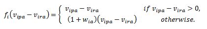
(1) - 3.6
- Note that each consumer agent has a unique value function because of its own attribute weight, wia. Similar to the study of Hardie et al. (1993), we adopt a linear value function as in equation (1), which is depicted in Figure 1. It is also possible to employ an S-shaped nonlinear function (Kahneman & Tversky 1979) that incorporates diminishing sensitivity to losses and gains for large differences, vipa− vira. However, the degree of diminishing sensitivity to losses and gains differs between cases (Abdellaoui et al. 2007). Because our focus is on modelling consumer behaviour using reference dependence and loss aversion rather than using diminishing sensitivity, we choose the linear function. The diminishing sensitivity is known as diminishing marginal utility and it means the marginal utility a person gets from adding another same product decreases as the number of products increases. However, our model only purchases one product. Therefore, we may not have to consider diminishing sensitivity.
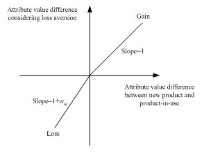
Figure 1. Loss aversion graph - 3.7
- The consumer agent i continues to revise its evaluation for each new product until it chooses a product or the simulation ends. Suppose that the new product p is entered into the market at simulation time t2. Let vipa t2 the biased evaluation value of the consumer agent at the time t2. Then, the consumer agent's biased value is initially set to
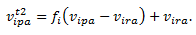
(2) At the simulation time t, which is greater than t2, the value is updated with the consideration of social influence as follows:
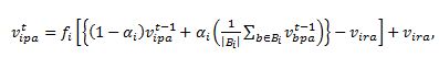
(3) where the Bi is the set of neighbours who are linked to the consumer agent i in the social network of consumer agents; the operator, |B i|, represents the size of the neighbour set; α i is the degree of the consumer agent's sensitivity to social influence. In this equation, 1/|B i|∑b∈Bi vbpa t-1 is the average social influence for the attribute a. We assume that all neighbouring agents influence the consumer agent i equally. To obtain the consumer agent's value, vipat, at the simulation time t with respect to attribute a, the value at time t-1, vipa t-1, and the average social influence are averaged with the consideration of the sensitivity to social influence, αi. Next, the value function is applied to obtain a new biased value at time t. Suppose that the consumer agent i has a negative value on the attribute a at the introduction time of the product p and that the agent is sensitive to social influence (i.e., αi is close to 1). Then, if the neighbours send several positive signals, the value will gradually shift in a positive direction – the agent becomes to favour the product attribute. Otherwise, our model makes the consumer agent's value continue to worsen. Gershoff et al. (2012) have discovered that a consumer feels unfairness when choosing a product if the product the consumer selected is inferior to its reference product which shares similar attributes or criteria for decision-making. And, such unfair feeling, which leads to a negative evaluation on the chosen product, can be mitigated by reducing similarity between the two products. For example, a consumer would value a cell phone lower when a reference product is a smart phone than when the reference product is a home phone. Because our model considers the competition of products sharing similar product attributes, we believe that a deteriorating value of a product by a consumer agent in our model represents a consumer's negative evaluation of unfairness.
- 3.8
- In the middle of a simulation run, the producer of a new product may desire to test the effect of a price discount on the sales volume. In this case, all consumer agents' values for attribute price should be modified positively at a discount time, such as t3. There are a few ways to reflect the impact of a price discount on the values of consumer agents. In our model, we change the value of attribute price as follows:
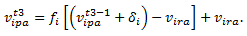
(4) In this equation, the attribute a represents price; vipat3-1 is the value of the attribute price endowed by the consumer agent i at time t3- 1; the δi is the unbiased value increment due to a price discount. We assume that δi is the same for all consumer agents. However, individual agents endow different biased values to the increment due to their unique value functions. The unbiased value increment, δi, is set to be proportional to the difference between the value upper bound of price attribute and the average value of all consumer agents assigned at the initialisation stage. For example, suppose that the producer offers a 10% price discount to the market. Then, if the value interval of the price attribute is [-4, 15] and the average value at the initialisation stage is 5, then δi = (15-5)·0.1=1. From the next simulation time, t = t3 + 1, the value of the consumer agent i is updated according to equation (3).
- 3.9
- Let vipt be the value of the product p evaluated by the consumer agent i at time t. Because there can be more than one product attribute, the personal total value, vipt, is the sum of attribute values of product p,
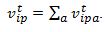
(5) - 3.10
- In general, a consumer buys a new product when some purchasing condition, such as utility maximisation, is met. In our model, for each simulation time t, each consumer agent compares its values on new products with a threshold and buys from the products a new one whose value is greater than the threshold, if it exists. We denote the initial threshold of consumer agent i by thresholdi0. The initial threshold is the sum of the attribute values of the reference product r, the product in use by the consumer agent i.
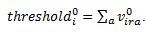
(6) - 3.11
- In general, the value of product in use depreciates over time (Feinschreiber 1969). Therefore, the threshold of the consumer agent i will decrease over time. In this study, a negative exponential function with a decay parameter, λ, is applied to model the decreasing process of the threshold:
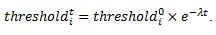
(7) In the equation, thresholdit is the threshold of the consumer agent i at simulation time t. Exponential decay is observed in a wide variety of disciplines such as economics and natural sciences (Feinschreiber 1969). The decay parameter, λ, takes a value within (0, 1]. A larger decay parameter implies faster depreciation and a shorter life cycle of a product family. Mobile phones including smartphone are, for instance, a representative product family with a short life cycle (Geyer & Blass 2010; Li et al. 2010).
- 3.12
- Let Pit denote the set of new products whose values evaluated by the consumer agent i exceed their thresholds at simulation time t. That is, Pit = {p| vipt > thresholdit}. We apply the multinomial logit model (McFadden 1974) to choose a product in Pit. This model is a widely applied product choice model (McFadden 1980; Guardagni & Little 1983; Villas-Boas & Winer 1999; Bentz & Merunka 2000). The multinomial logit approach models the effect of product attributes on probability of choice with a logit formulation. According to the multinomial logit model, the consumer agent i chooses a new product among the candidates in Pit at simulation time t as
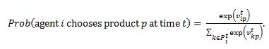
(8) As stated previously, some consumer agents will not buy new products at the end of a simulation run if their thresholds remain higher than the values of all new products. In our model, these are regarded as non-adopters.
Experiments
-
Objective
- 4.1
- Netlogo (Wilensky 1999), a well-known computer program for agent-based modelling, was used to implement our model. We conducted two experiments in this study. In both experiments, we considered the mobile phone market in Korea in which three major new products – two smartphones and one convergence product – compete with each other. The three products belong to a high-tech but fashionable product family. Therefore, those products usually have short life cycles compared to durable goods, such as 1–2 years. The two smartphones are provided by two different producers and account for 80% of the Korean smartphone market. The convergence product is a smartphone sharing some features of tablet PCs. It is the most popular one among similar convergence products sold in Korea and provided by one of the two producers. We also focused on the urban young people segment in the market because they are the most active and critical segment for producers seeking to understand market behaviour. Urban young people are skilled in handling smartphones and put forth their opinions widely through social networking services.
- 4.2
- The first experiment is sensitivity analysis on the product life cycle and social influence. In our model, the decay parameter of the product in use becomes short as the life cycle of new product decreases, and social influence strengthens as the degree of sensitivity to social influence increases. The objective is to observe how consumer agents behave as the decay parameter and the degree of sensitivity change. The second experiment is sensitivity analysis on time-to-market, time-to-discount, and amount-to-discount. The optimal combination of the three marketing strategies that maximises the sales volume (or revenue) of the new convergence product is sought from the sensitivity analysis. Based on our results, we provide pricing and timing implications for firms, aiming to increase sales volumes (or revenue) from their products.
Setup
- 4.3
- To implement our model, samples of urban young Koreans were asked to answer a questionnaire. They were asked to rate 15 product attributes, selected as key determinants of product purchase by the Korea Information Society Development Institute (Park et al. 2011), of new products as well as products in use. Brand loyalty, price, display size, and the number of applications were chosen from the 15 product attributes. They were selected by calculating the variance of each product attribute. A product attribute of high variance means it can classify people into groups. The four attributes are the top-four high-variance product attributes.
- 4.4
- In the sample survey, the urban young people were asked to rate the attributes of products in use (i.e., reference products) within a range of [1, 10], as shown in the second row of Table 1. They also rated the attributes of the three new products with respect to their references within a range of [−5, 5]. That is, the attribute value of a new product is set relatively better or worse than the attribute value of a reference product. Therefore, the attribute value of a new product becomes a number within [−4, 15]. Table 1 shows the means and the standard deviations of the four attributes of the Reference product (product in use), Product 1 (a smartphone), Product 2 (a smartphone), and Product 3 (convergence product). The numbers in parentheses are the standard deviations. A higher mean implies a more satisfactory corresponding product attribute. Product 2 is thought to be the most satisfactory product in price. Product 2 and Product 3 are highly valued in display size. The number of applications is high in Product 1. For all product attributes, one product does not perfectly overwhelm the other products. Therefore, consumer agents' evaluation processes and social interactions will matter for choosing new products.
Table 1. The means and the standard deviations of four attributes of Reference, Product 1, Product 2, and Product 3 (convergence product) 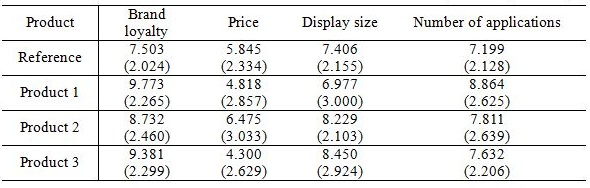
- 4.5
- Table 2 summarises linguistic evaluation for weights of the four product attributes. The numbers of samples rating brand loyalty, price, display size, and the number of applications as "High" or "Very high" were 63, 75, 70, and 58, respectively. This finding indicates that over half of the samples have a high degree of loss aversion for the four product attributes. In addition, the number of samples rating brand loyalty, price, display size, and the number of applications as "Very high" were 17, 40, 17, and 26, respectively. This finding implies that urban young Koreans treat price as the most important product attribute. Note that, from Table 1, Product 2 is the most satisfactory product in terms of price. Table 3 presents an empirical distribution of sensitivity to social influence. The distribution is right-skewed. We may guess that urban young Koreans are sensitive to others' evaluation opinions on smartphones.
- 4.6
- We assume that the input variables of weight and sensitivity to social influence are fuzzy variables whose values can be obtained from sample survey. Fuzzy set theory supports an effective way to quantify the linguistic terms of fuzzy variables. The ambiguity of each term in this study is classified as a value set with a triangular membership functions (Zimmermann 2001). For example, a value set of (0, 0, 0.5) is defined as a triangular fuzzy number. The corresponding membership function implies how much certain a value in the set is classified as a linguistic term. Triangular fuzzy numbers for a specific application domain can be drawn by using survey data (Hong & Lee 1996). However, drawing triangular fuzzy numbers remains a challenging problem. We also assume that we can transform a triangular fuzzy number into a crisp number by applying the graded mean integration representation method used in Kim et al. (2011). For more details in fuzzy numbers, refer to Appendix.
- 4.7
- Table 2 shows the linguistic terms for a weight of a product attribute, and the frequencies of linguistic terms responded for each product attribute. For more details of the linguistic terms, refer to Table A in Appendix. The numbers of samples rating Brand Loyalty, Price, Display Size, and Number of applications as "High" or "Very High" were 63, 75, 70, and 58, respectively. It means that the four product attributes are important for the samples. And, the numbers of samples rating Brand Loyalty, Price, Display Size, and Number of applications as "Very High" were 17, 40, 17, and 26, respectively. It implies that Korean urban young people treats Price as the most important product attribute. We may guess this is because they are too young and needy to afford new products. They also treat Brand loyalty and Display size important rather than Number of applications. Since Brand loyalty and Display size decide the social image of a product and Number of applications determines the utilization of a product, we may suspect that Korean urban young people care more about social image obtaining from products than about usage of the products.
- 4.8
- Table 3 shows a discrete distribution of sensitivity to social influence of the samples in linguistic terms (For more details of the linguistic terms, refer to Table B in Appendix). The histogram of this distribution will be right-skewed. This means the samples are sensitive to social influence when buying new products. We may guess that Korean urban young people are sensitive to others' opinion on products.
Table 2. Frequencies of weights in linguistic terms for each product attributes 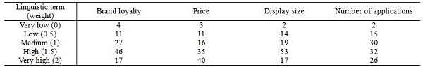
Table 3. Frequencies of linguistic terms for sensitivity to social influence 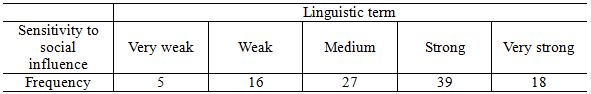
Sensitivity analysis on product life cycle and social influence
- 4.9
- First, we conducted a sensitivity analysis on the decay parameter to observe how Korean urban people change their behaviour when the life cycles of new products become longer or shorter than the current setting, 15 months. In Korea, the interval between the releases of a smartphone and its upgraded version varies, usually between 12 and 24 months. The decay parameter of 0.1 corresponds to a life cycle of approximately 15 months. The perturbation was employed by setting the life cycle to 12 months and 18 months to consider the shorter and the longer life cycles, respectively. The values of the decay parameter for both life cycles are 0.13 and 0.075, as shown in Table 4.
- 4.10
- In Figure 2, the order of sales volumes of the three products remains the same regardless of the change of the decay parameter. In this figure, a time step corresponds to a month. The order coincides with the order of the sums of mean attribute values in Table 1 (i.e., Product 2, Product 1, and Product 3, whose sums of mean attribute values are 31.427, 30.432, and 29.763). This finding implies that the change in the life cycle of products may affect the sales volume of the products slightly. However, we may observe that small differences in evaluations among the three products lead to large differences in the sales volumes of the products. For example, the sum of the mean values of product attributes of Product 2 differs from that of Product 3 by approximately 1.5. However, the difference between the sales volume of Product 2 and that of Product 3 is approximately 100. We may guess that properties of reference dependence and loss aversion in product evaluation lead more urban young Koreans to buy the superior product, even though the evaluation difference between the superior product and the inferior product is small.
- 4.11
- Table 5 presents the final sales volumes of the three products with respect to the decay parameter. Each entry in the table was drawn from averaging the final sales volumes of 100 simulation runs. As the decay parameter decreases (i.e., the expected life cycle increases), Product 2 earns sales volumes, but Product 1 and Product 3 lose sales volume. This result occurs because a longer life cycle guarantees that a better product (Product 2 in this case) will have enough time to spread good opinions on the product and that a worse product (Product 1 or Product 3 in this case) will have sufficient time to be revealed as an inferior product relative to the better product (Lee et al. 2013). Alternatively, a worse product obtains an advantage of sales volume from a shorter product life cycle, whereas a better product obtains a disadvantage in sales volume from a shorter life cycle.
Table 4. Expected life cycle in month with respect to a decay parameter 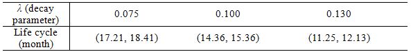
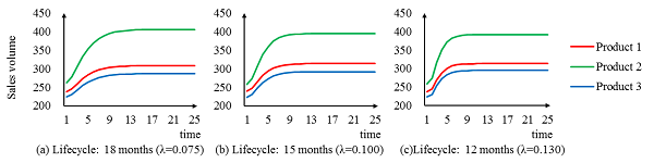
Figure 2. Sales volumes of three products with respect to decay parameter Table 5. Final sales volumes of three products with respect to decay parameter 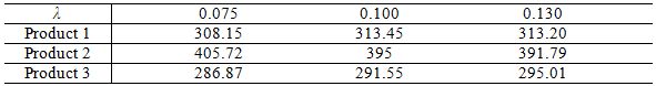
- 4.12
- Second, we conducted a sensitivity analysis on social influence to observe how urban young Koreans alter their behaviour when they become more or less susceptible to WOM than the present setting, as in Table 3. The life cycle of the three products was fixed at 15 months (i.e., λ is 0.1). We perturbed the empirical probability distribution of the sensitivity to social influence in Table 3. Table 6 shows the final sales volumes of the three products with respect to changes in the distribution. The final sales volumes were calculated by averaging the final sales volumes of 100 simulation runs. In the table, "Default" in the top row represents the original empirical distribution. "Weaker" refers to the distribution made by shifting 30% samples of "Medium", "Strong", and "Very strong" categories in Table 3 to the next-left categories. This treatment indicates that consumers are less sensitive to social influence than the default setting. "Stronger" is the distribution made by shifting 30% samples of "Medium", "Weak", and "Very weak" categories in Table 3 to the next-right categories. This shift makes consumers more sensitive to social influence than the default setting.
Table 6. Final sales volumes of three products with respect to sensitivity to social influence 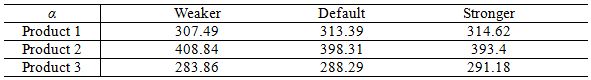
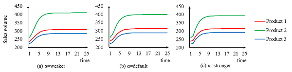
Figure 3. Sales volumes of three products with respect to the distribution of sensitivity to social influence - 4.13
- Intuitively, a better product should obtain an advantage in sales volume as consumers become more sensitive, just as when a long life cycle provides enough time for the better product to be known as superior. However, in our experiment, not a better product (Product 2) but a worse product (Product 1 or Product 3) had an advantage in sales volume. As sensitivity to social influence increases, the sales volumes of Product 1 and Product 3 increase by 7 and 9, respectively. Meanwhile, the sales volume of Product 2 is reduced by 15.
- 4.14
- We may guess that the difference between the evaluations of the better product and the worse product decreases as consumer agents become more sensitive to social influence. As seen in the Figure 4, the difference between the mean values of 1000 agents' evaluation on Product 1 when agents are more sensitive to social influence and that of 1000 agents' evaluation on Product 1 when agents are less sensitive to social influence is −0.1 in the end. The corresponding values for Product 2 and Product 3 are −0.25 and −0.1, respectively. Namely, as agents get more sensitive to social influence, agents' evaluation on all the products becomes lower. However, the better product, Product 2, loses more values than the others in total. This provides relative advantages to the worse products, Product 1 and Product3. And thus, agents are likely to choose Product 1 and Product 3 rather than Product 2 according to Equation (8), so that the sales volumes of Product 1 and Product 3 have increased and the sales volume of Product 2 has decreased as in Table 6.
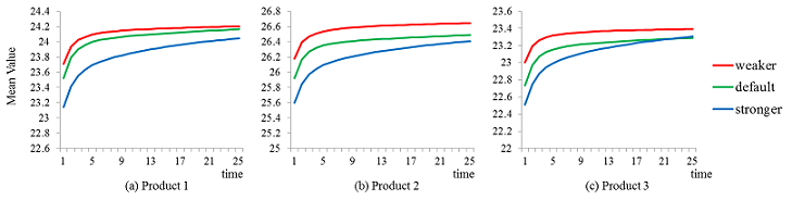
Figure 4. Mean values of three products over time with respect to the distribution of sensitivity to social influence 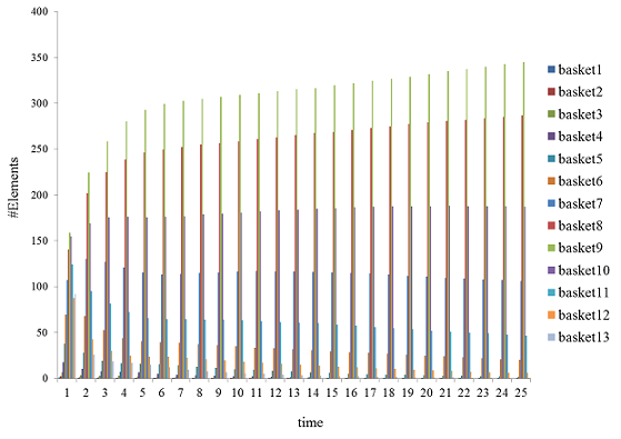
Figure 5. Numbers of elements in 13 baskets over time when the sensitivity to social influence is stronger than default case (In case of Product 2) - 4.15
- We suspect that this result is due to the averaging effect of WOM. As the sensitivity to social influence increases, consumer agents are likely to rely on social evaluation transmitted through social networks rather than personal evaluation. Whereas the personal evaluation varies highly due to the initial random assignments, integrating neighbours' evaluation extenuates the variety in personal values. For example, Figure 5 shows the numbers of elements in 13 baskets over time, when the sensitivity to social influence is stronger than default case. Here, we have clustered all the agents' values on criteria 1 of Product 2 into 13 groups. For each time, a histogram is induced with 13 clusters. We can verify that the histogram gets narrower as time flows. It means that the values converge into a certain point, an average, because of social interaction, WOM. Such averaging effect of WOM happens in any case of this sensitivity analysis. And such effect happens in all the other criteria and products.
- 4.16
- Such a phenomenon often happens in practice. One case may be the increase in the variety of products but a decrease in the number of monopolies in recent years due to a stronger stimulation of many communication channels. We are now experiencing fewer monopolies than in the past because many communication channels, including the mass media, social media, and micro media provide more information on various products to consumers than before.
Sensitivity analysis on time-to-market, time-to-discount, and amount-to-discount
- 4.17
- In this experiment, we controlled time-to-market, time-to-discount, and amount-to-discount to observe how urban young Koreans react to marketing strategies (i.e., timing and pricing) of the producer of Product 3, a new convergence product. Because the producer must bear the failure risk of the new convergence product, marketing strategies that can create market share of the product are important to the producer. We assume that the introduction times of Product 1 and Product 2 are the same and that the producer of Product 2 is planning to launch a new convergence product (Product 3) that may compete with Product 1 and Product 2. The time-to-market varied from one month before to five months before the introduction of Product 1 and Product 2. The time-to-discount was changed from the release time of Product 3 to five months after the time. The amount-to-discount was set to a rate from 0% to 50% in increments of 10%.
- 4.18
- Figure 6 shows the sales volume of Product 3 with respect to the release time, discount time, and discount rate of the product. In this figure, the entries in each table are the final sales volumes of Product 3 in an average of 100 simulation runs. This figure also supports a corresponding contour map within each table. The numbers in the leftmost column in each table indicate the time of the discount. For example, in Table (c) of Figure 6, the number, −2, on the leftmost column indicates a price discount on Product 3 applied 2 months before the launches of the other products. The numbers on the top row in each table represent discount rates. Even though there is no discount in a column where the discount rate is 0% in each table, the final sales volumes differ. For example, Table (e) of Figure 6 shows values of 750.1, 747.1, 748.4, 749.3, 749.0, and 749.4. The differences among the sales volumes were caused by randomness in the product choice of each consumer agent in Equation 8.
- 4.19
- In Figure 6, an earlier release with a higher discount rate and an earlier discount time produces the maximum sales volume of Product 3. This finding is easily confirmed by examining contour maps in Figure 6. The results ensure that the proposed simulation model represents general phenomena expected in practice very well. In specific, given the same discount rate and discount time, the earlier release of Product 3 appears to make Product 3 dominate the market share and to lock consumers in Product 3. For instance, given a discount rate of 50% and a discount time of 0, the sales volume of Product 3 increases as the release time is set earlier – the sales volume is 421.0 when the release time is 0, 653.0 when the release time is −1, 660.5 when the release time is −2, 717.3 when the release time is − 3, 779.1 when the release time is −4, and 832.4 when the release time is −5. We may suppose that an early release of Product 3 builds a lock-in effect by early adopters of Product 3 as well as sufficient social influence to hold a dominant position.
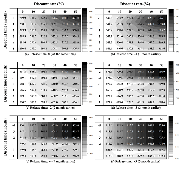
Figure 6. The final sales volume of Product 3 with respect to discount time and discount rate: (a) when release time is 0, (b) when release time is −1, (c) when release time is −2, (d) when release time is −3, (e) when release time is −4, and (f) when release time is −5 - 4.20
- Given the same release time and discount time, the sales volume of Product 3 increases as the discount rate increases. We may confirm this result by examining every table of Figure 6 from left to right. For example, given the release time by −3 and the discount time by −2 in Figure 6 (d), the sales volumes with discount rates of 0%, 10%, 20%, 30%, 40%, and 50% are 674.9, 729.5, 794.1, 845.4, 887.8, and 917.7, respectively. We believe that a higher discount rate stimulates consumers to purchase Product 3.
- 4.21
- When fixing the discount rate and the release time, we observe that the sales volume becomes higher or remains the same when the discount time is over a month earlier than the other products' releases. For example, in Figure 6 (e), where the release time is −4, when the discount rate is fixed as 10 %, the sales volumes with discount times of −3, −2, and −1 are 810.3, 805.6, and 806.7, respectively. Meanwhile, those with discount times of 0, 1, and 2 are 741.6, 755.4, and 753.8, respectively. That is, the sales volume decreases as the discount time is moved later than the other products' releases.
- 4.22
- Tables in Figure 6 were converted into graphs in Figure 7, in which each path shows a sales volume change with respect to the discount rate for a discount time. At a macroscopic level, the meanings of graphs in Figure 7 and tables in Figure 6 are the same – an earlier release, earlier discount time, and larger discount rate facilitate an increase in the sales volume of Product 3. However, we have three new findings from Figure 7 at a microscopic level.
- 4.23
- The first finding is that paths in each graph of Figure 7 may be classified into two groups as the release time of Product 3 is moved earlier. This phenomenon is clear in graphs (c), (d), (e), and (f) of Figure 7. In those graphs, paths of discount times less than −1 (i.e., one month earlier than the release time of the other products) grow substantially relative to the others. This finding indicates that Product 3 obtains an advantage of a monopoly with a strong social influence when discounting its price at least two months earlier than the introduction of the other products. Many potential adopters would buy Product 3 during a monopoly period because of the stimulation of a price discount and, as a result, few consumers were left before the introduction of the other products. In these graphs, a price discount close to or later than the release of the other products is not effective. Such a phenomenon is not seen in graphs (a) and (b), in which the release time is almost the same as that of the other products. Overall, an earlier product release and discount time is very desirable for increasing the sales volume of Product 3.
- 4.24
- The second finding is that, as shown in concave paths in graphs (c), (d), (e), and (f) of Figure 7 in which release time is earlier than −1 (for example, paths for discount times of −2, −3, −4 and −5 when the release time is −5), the marginal sales volume decreases with respect to the discount rate. In these graphs, the diminishing degree of the marginal sales volume increase is more prominent as the release time is moved earlier. An early product release certainly creates a monopoly effect with a strong social influence and high discount rate also stimulating non-adopters to buy Product 3. However, an excessive discount rate does not increase the sales volume as expected (e.g., a linear increase) because some non-adopters who prefer Product 1 or Product 2 remain regardless of the high discount rate of Product 3. This phenomenon implies that the producer of Product 3 should pay special attention to choose the discount rate because a discount rate that is too high may result in a low profit.
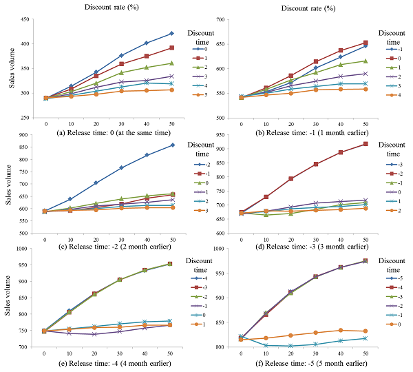
Figure 7. The final sales volume of Product 3 with respect to the discount rate for each discount time rate: (a) when the release time is 0, (b) when the release time is −1, (c) when the release time is −2, (d) when the release time is −3, (e) when the release time is −4, and (f) when the release time is −5 - 4.25
- It is a common expectation that the sales volume of Product 3 increases more as the discount time is moved earlier. However, our third finding from the experiment is that the order of sales volumes between a discount time of −1 and a discount time of 0 (i.e., discount is applied when other products are introduced) is reversed in all graphs in Figure 7. For better understanding, we monitored traces of simulation runs when the release time of Product 3 is −3 and its discount rate is 20%. Table 7 summarises a partial trace from a runtime of step −3 to 3.
Table 7. The sales volumes of Product 3 over time when its introduction time is 3 months earlier than the other products and its discount rate is 20% (from its introduction to third months from the introductions of the other products) 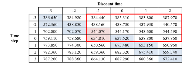
- 4.26
- In Table 7, each column indicates the sales volume of Product 3 over time with respect to a discount time. From six small boxes in the table, we know that the price discount appears to be effective in increasing the sales volume of Product 3 – for instance, when the discount time is −2, the sales volumes increase between the time steps −2 and −1 is 438.85−702.07=263.22. However, in the large box outlined in red, we notice that numbers of the third column (i.e., when discount time is −1) and those of the fourth column (i.e., when discount time is 0) are similar until the time step is 0 (i.e., before the other products are released). In addition, the numbers in the fifth and the sixth columns until the time step 0 are similar to those in the third and the fourth columns. From the observation, we know that results with similar increases in sales volume are caused solely by monopolistic social influence from Product 3's early release. Therefore, in the case of the third column, where a price discount on Product 3 is given on time step −1, the price discount effect for a sales volume increase disappears due to the strong social influence. This interesting finding gives us an implication that a product's early discount time close to the release time of competing products does not contribute to increase the sales volume of the product significantly, when the product currently holds a monopolistic position in a market and the competing products are to be released soon. Rather, it is desirable to offer a price discount much earlier or later than the introduction of competing products.
- 4.27
- Furthermore, by knowing that one producer manufactures Product 2 and Product3, we can find a conflict in the market share between the sales volumes of Product 2 and Product 3 – as Product 3 gained more market share by using marketing strategies, Product 2 lost more market share. For the producer of Product 2 and Product 3, searching the optimal discount time, discount rate, and release time of Product 3 that achieves the maximum revenue in such a trade-off situation is important. Figure 8 illustrates the revenue of the producer of Product 2 and Product 3 with respect to the discount time, discount rate, and release time of Product 3. To calculate the revenue, we have used the real sales prices of the three products in June 2012. The prices of Product 1, Product 2, and Product 3 were 500,000, 200,000, and 490,000 Korean won, respectively.
- 4.28
- For every release time of Product 3, the minimum revenue occurred in two conditions. One condition is when the price discount rate of Product 3 is 10% or 20%. The other condition is when the price discount on Product 3 is set one month earlier than the release times of the other products. A low discount rate and discount time of Product 3 right before the releases of the other products led to low revenues for the producer. As seen in the previous analysis, the discount time of -1 led to a small sales volume of Product 3. Therefore, an early discount time close to the introduction of Product 1, a competing product of a different producer, with a low discount rate gave the producer of Product 1 the chance to increase its sales volume. Therefore, if Product 3 is planned for release at a discount time of −1, if possible, the producer should offer a discount of more than 20% to raise revenue or may have to avoid the discount time of −1.
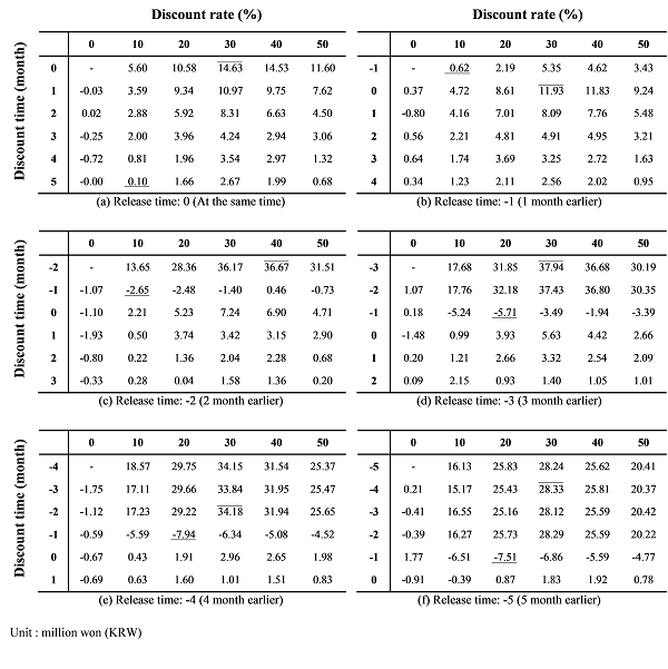
Figure 8. The revenue of the producer of Product 2 and Product 3 with respect to the discount time and discount rate: (a) when the release time is 0, (b) when the release time is −1, (c) when the release time is −2, (d) when the release time is −3, (e) when the release time is −4, and (f) when the release time is −5 - 4.29
- On the contrary, the maximum revenue was achieved when the discount rate of Product 3 was 30% or 40%. Regardless of the release time and the discount time of Product 3, the discount rate of 30% (or 40% in the case of a release time of −2) guaranteed the maximum revenue for the producer. A high discount rate that was not extreme (e.g., a 50% discount) resulted in a high sales volume of Product 3 with the greatest revenue for the producer. In addition, when the release time of Product 3 is set earlier than one month before the release times of the other products (i.e., tables (c), (d), (e), and (f) of Figure 8), the discount time should be over a month earlier than the release times of the other products. This result implies that enough time for dominant social influence on Product 3 is required to improve the revenue of the producer (in this case, two months or more). To maximise revenue when a producer introduces a new high-profit convergence product (e.g., Product 3) and sells a product similar to but less profitable than the convergence product (e.g., Product 2), the producer should not only release the new convergence product but also give a price discount as early as possible. In addition, the rate of the price discount should not be too high or too low. However, an exception is observed when the release time of Product 3 is 0 or −1 (i.e., tables (a) and (b) of Figure 8). In such a condition, the maximum revenue is achieved with a discount time of 0. This special case implies that the price discount should be offered at the same time of the release of competitive products (e.g., Product 1) if technological problems make the release time of the new convergence product very close to the release times of competitive products. The producer does not have enough time to create a dominant social influence for the new convergence product.
Conclusion
- 5.1
- Firms are struggling in a competitive market environment. A successful launch of a new product necessitates firms' understanding about the diffusion dynamics of the product as well as competing products to employ appropriate marketing strategies such as timing and pricing. In this study, we addressed pricing and timing strategies of a new product by developing an agent-based product diffusion simulation. In recent years, agent-based modelling has emerged as a good instrument for studying complex social and economic phenomena. This technology is capable of investigating how macro diffusion dynamics arise from individual decisions of many consumers and how the resulting dynamics feed back to the individual decision making of potential adopters.
- 5.2
- In general, consumers are not perfectly rational when they choose new products – they are accustomed to evaluating a new product by comparing it with their products in use as references and most feel losses more severe than gains, even when the amounts are the same. In this study, we modelled consumers' behaviours of reference dependence and loss aversion and built an agent-based simulation in which the diffusion dynamics of competing products emerge from the aggregation of consumers' individual decisions. In the proposed simulation model, agents imitate behavioural consumers who are reference dependent and risk averse in the evaluation of new products and their interactions create word-of-mouth about new products, which affects the product choice of potential adopters.
- 5.3
- The proposed simulation model was applied to the Korean mobile phone market, in which urban young people, who are strongly sensitive to social influence, are the most critical market segment. According to our findings, young Koreans are more likely to buy a superior product as the life cycles of the product family increase. We find this result because a longer life cycle leads a superior product to have enough time to spread good opinions on the product throughout social networks. However, these people are likely to purchase an inferior product as they become more sensitive to social influence. We suspect that this result is due to the averaging effect of word-of-mouth. As the sensitivity to social influence increases, consumer agents are more likely to rely on social evaluation transmitted through social networks rather than on personal evaluations. Whereas personal evaluations vary highly, integrating neighbours' evaluation attenuates this variety.
- 5.4
- Focusing on time-to-market, time-to-discount, and amount-to-discount, we induce pricing and timing implications from the perspective of the sales volume of a new convergence product and the revenue of the producer who also released a typical mobile phone in the market. According to our result, an earlier release with a higher discount rate and an earlier discount time ends with the maximum sales volume of the new convergence product. Specifically, the firm must introduce the product and provide a discount on the product at least two months earlier than competitors' product introduction. Because Korean young people are reference dependent and loss averse, a short period of time, such as one month, cannot effectively increase the sales volume of the product. If the firm produces a new convergence product as well as a typical product, there exists a trade-off between the sales volumes of the two products. A high but not extreme discount rate results in a high sales volume of the convergence product with the greatest revenue for the firm, regardless of the release time and the discount time. On the contrary, a low discount rate and discount time right before the releases of other products lead the firm to obtain minimal revenues.
- 5.5
- In the future, we plan to investigate the following issues:
- An analysis of variance on time-to-market, time-to-discount, and amount-to-discount is necessary to analyse interaction effects on changes in sales volume.
- A thorough validation of the agent-based model based on prospect theory is necessary. This study concentrated on the application of the model to the timing and pricing of a new product. However, the predictive power of the model should be further validated by comparing with the model constructed on the basis of conventional utility maximisation principle with more real diffusion data.
Pseudo code
-
Function main [lambda]
For each time-to-market
For each time-to-discount
For each amount-to-discount
For each replication
setup [lambda]
simulate
End
Function setup [lambda]
setup-globals [lambda]
make-consumers
assign-agent-attribute
make-init-neighbors
rewire-neighbors
renew-links
End
Function make-consumers
Create some given number of consumers
End
Function setup-globals [lambda]
Assign 0 to time step
Assign lambda to decay parameter
Assign 0 to adopter number for each product
Assign crisp numbers to consumer's linguistic weights on products attributes
Assign the probability of consumer's sensitivity to social influence in linguistic form
End
Function assign-agent-attribute
For each consumer agent
Assign random values to products' attributes
Retrieve consumer's weights on products' attributes randomly
Convert consumer's weights on products' attributes into crisp numbers using triangular fuzzy number
Retrieve consumer's sensitivity to social influence randomly
Convert consumer's sensitivity to social influence into crisp numbers using triangular fuzzy number
Assign sum of value of reference product attributes to total value of reference product
End
Function make-init-neighbors
For each consumer agent
Assign neighbors as many as the degree of connectivity
End
Function rewire-neighbors
For each consumer agent
Connect to its own neighbors
Rewire the connections in probability of rewiring probability
End
Function renew-links
For each consumer agent
if the number of connections is NOT equal to the degree of connectivity
Add/Delete connections until the number of connections is equal to the degree of connectivity
End
Function simulate
get-socio-influence
get-prospected-value-of-new-products
get--value-of-products
update-threshold
buy-product
End
Function calculate-value-function [attribute value of new product - attribute value of reference product, weight of attribute]
If attribute value of new product - attribute value of reference product is bigger than 0
Return attribute value of new product - attribute value of reference product
Else
Return (1 + weight of attribute) * (attribute value of new product - attribute value of reference product)
End
Function get-socio-influence
For each consumer agent
For each released products
For each attributes
Retrieve all the neighbors' attribute value and average them
Reassign attribute value by (1 - sensitivity to social influence) * my attribute value + (sensitivity to social influence * the averaged attribute value of all the neighbors)
End
Function get-prospected-value-of-new-products
For each consumer agent
For each released products
For each loss aversive attributes
Retrieve weight of attribute
If attribute is price
Retrieve amount-to-discount
Reassign attribute value by calculate-value-function [attribute value of released products + amount-to-discount - attribute value of reference product, weight of attribute] + attribute value of reference product
If attribute is not price
Reassign attribute value by calculate-value-function [attribute value of released products - attribute value of reference product, weight of attribute] + attribute value of reference product
End
Function get--value-of-products
For each consumer agent
For each released products
Assign sum of value of new product attributes to total value
End
Function update-threshold
For each consumer agent
Retrieve decay parameter
Retrieve time step
Assign total value of reference product ^ (- decay parameter * time step) to threshold
End
Function buy-product
For each consumer agent
For each released products
Buy a product according to multi-nomial logit model
End
Appendix Triangular fuzzy number
-
Fuzzy set theory supports an effective way to quantify the linguistic terms of fuzzy variables. The ambiguity of each term in this study is classified as a value set with a triangular membership functions (Zimmermann 2001) as in Figure A. As in Figure B, a value set of (a,b,c) is called triangular fuzzy number. The corresponding membership function implies how much certain a value in the set is classified as a linguistic term. We define triangular fuzzy numbers for weight on a product attribute and sensitivity to social influence in five scales.
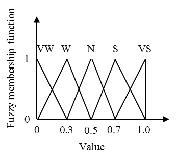
Figure A. The fuzzy member function of Table A 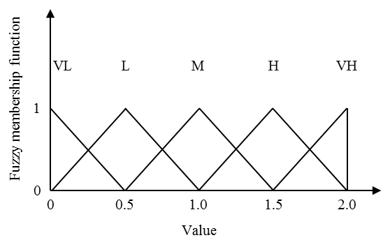
Figure B. The fuzzy member function of Table B 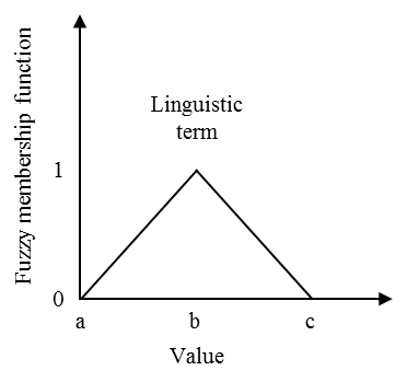
Figure C. A depiction of a triangular fuzzy number Table A. Linguistic terms of weight and corresponding triangular fuzzy number 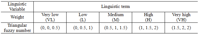
Table B. Linguistic terms of sensitivity to social influence and corresponding triangular fuzzy number 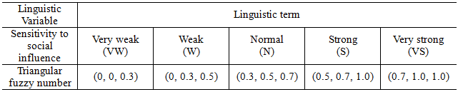
We apply the graded mean integration representation method (Chou 2003) which provides easier understanding and simpler calculation for triangular fuzzy number with a scalar. The methods converts a fuzzy number into a crisp value as follows (refer to Chou (2003) for more detail).
Definition. The graded mean integration representation method transforms a triangular fuzzy number X = (x1, x2, x3) into a crisp number P(X) by
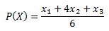
(a)
Acknowledgements
- This research was supported by the Basic Science Research Programme through the National Research Foundation of Korea (NRF) funded by the Ministry of Education (2010-0009267,NRF-2013R1A1A2A10013104) and Ministry of Science, ICT & Future Planning (NRF-2012R1A1A2046061), and by the Korea Foundation for the Advancement of Science & Creativity (KOFAC) grant funded by the Korean Government (MEST).
References
-
ABDELLAOUI, M., Bleichrodt, H., & Paraschiv, C. (2007). Loss aversion under prospect theory: a parameter-free measurement. Management Science, 53, 1659–1674. [doi:10.1287/mnsc.1070.0711]
BARBERIS, N., Huang, M., & Santos, T. (2001). Prospect theory and asset prices. Quarterly Journal of Economics, 116(1), 1–53. [doi:10.1162/003355301556310]
BASS, F.M. (1969). A new product growth model for consumer durables. Management Science, 15(5), 215-227. [doi:10.1287/mnsc.15.5.215]
BEGGS, A., & Graddy, K. (2009). Anchoring effects: evidence from art auctions. American Economic Review, 99(3), 1027–1039. [doi:10.1257/aer.99.3.1027]
BENTZ, Y., Merunka, D. (2000). Neural Networks and the Multinomial Logit for Brand Choice Modelling: a Hybrid Approach. Journal of Forecasting, 19, 177–200. [doi:10.1002/(SICI)1099-131X(200004)19:3<177::AID-FOR738>3.0.CO;2-6]
BLEICHRODT, H., Pinto, J.L., Wakker, P.P. (2001). Making Descriptive Use of Prospect Theory to Improve the Prescriptive Use of Expected Utility. Management Science, 47(11), 1498–1514. [doi:10.1287/mnsc.47.11.1498.10248]
BROMILEY, P. (2009) A Prospect theory model of resource allocation. Decision Analysis, 6(3), 124–138. [doi:10.1287/deca.1090.0142]
CAMERER, C., & Thaler, R. H. (1995). Anomalies: ultimatums, dictators and manners. The Journal of Economic Perspectives, 9(2), 209–219. [doi:10.1257/jep.9.2.209]
CAMERER, C.F. (2008). Neuroeconomics: opening the gray box. Neruon, 60(3), 416–419. [doi:10.1016/j.neuron.2008.10.027]
CHAPMAN, G.B., & Johnson, E.J. (2002). Incorporating the irrelevant: anchors in judgements of belief and value. In T. Gilovich, D. Griffin, & D. Kahneman (Eds.), Heuristics and Biases: The psychology of Intuitive Judgement (pp. 120–138). Cambridge: Cambridge University Press. [doi:10.1017/CBO9780511808098.008]
CHOU, C,-C. (2003). The canonical representation of multiplication operation on triangular fuzzy numbers. Computers and Mathematics with Applications, 45, 1601–1610. [doi:10.1016/S0898-1221(03)00139-1]
DAVIS, F.D., Bagozzi, R.P., & Warshaw, P.R. (1989). User Acceptance of Computer Technology: A Comparison of Two Theoretical Models. Management Science, 35(8), 982–1003. [doi:10.1287/mnsc.35.8.982]
DAVIS, F. D. (1986). A Technology Acceptance Model for Empirically Testing New End-User Information Systems: Theory and Results. Doctoral dissertation, Sloan School of Management, Massachusetts Institute of Technology.
DELRE, S.A., Jager W., & Janssen, M.A. (2007a). Diffusion dynamics in small-world networks with heterogeneous consumers. Computational and Mathematical Organization Theory, 13, 185–202. [doi:10.1007/s10588-006-9007-2]
DELRE, S. A., Jager, W., Bijmolt, T. H. A., & Janssen, M. A. (2007b). Targeting and timing promotional activities: an agent-based model for the takeoff of new products. Journal of Business Research, 60(8), 826–835. [doi:10.1016/j.jbusres.2007.02.002]
[doi:10.1016/j.sepro.2011.10.024]
DIAO J., Zhu, K., & Gao, Y. (2011). Agent-based simulation of durables dynamic pricing. Systems Engineering Procedia, 2, 205–212. [doi:10.2307/2490263]
FEINSCHREIBER, R. (1969). Accelerated depreciation: a proposed new method. Journal of Accounting Research, 7(1), 17–21.
FISHBEIN, M. & AJZEN, I. (1975). Belief, Attitude, Intention and Behaviour: An Introduction to Theory and Research, Addison-Wesley, Reading, MA. [doi:10.1162/003355301753265561]
GENESOVE, D., & Mayer, C. (2001). Loss aversion and seller behaviour: evidence from the housing market. Quarterly Journal of Economics, 116(4), 1233–1260. [doi:10.1086/663777]
GERSHOFF, A.D., Kivetz, R., & Keinan, A. (2012). Consumer response to versioning: how brands' production methods affect perceptions of unfairness. Journal of Consumer Research, 39(2), 382–398. [doi:10.1007/s00170-009-2228-z]
GEYER, R., & Blass, V.D. (2010). The economics of cell phone reuse and recycling. International Advanced Manufacturing Technology, 47, 515-525. [doi:10.1287/mksc.1040.0071]
GODES, D., & Mayzlin, D. (2004). Using Online Conversations to Study Word-of-Mouth Communication. Marketing Science, 23(4), 545–560. [doi:10.1287/mksc.2.3.203]
GUARDAGNI, P., & J. Little. 1983. A logit model of brand choice calibrated on scanner data. Marketing Science, 2, 203–238. [doi:10.1057/jors.2009.170]
GUNTHER, M., Stummer, C., Wakolbinger, LM, & Wildpaner, M. (2011). An agent-based simulation approach for the new product diffusion of a novel biomass fuel. Journal of the Operational Research Society, 62, 12–20. [doi:10.1287/mksc.12.4.378]
HARDIE, B.G.S., Johnson, E.J., & Fader, P.S.(1993). Modeling loss aversion and reference dependence effects on brand choice. Marketing Science, 12(4), 378-394. [doi:10.1007/s10683-008-9203-7]
HARRISON, G.W., & Rutström, E.E. (2009). Expected utility theory and prospect theory: one wedding and a decent funeral. Experimental Economics, 12, 133–158. [doi:10.1287/mnsc.1100.1269]
HE, X.D., & Zhou, X.Y. (2011). Portfolio choice under cumulative prospect theory: an analytical treatment, Management Science, 57(2), 315–331. [doi:10.1016/0165-0114(95)00305-3]
HONG, T-P., & Lee, C-Y. (1996). Induction of fuzzy rules and membership functions from training examples. Fuzzy Sets and Systems, 84, 33–47. [doi:10.1016/j.jbusres.2007.02.003]
JAGER, W. (2007). The four P's in social simulation, a perspective on how marketing could benefit from the use of social simulation, Journal of Business Research, 60, 868–875. [doi:10.1162/106454603322694807]
JANSSEN, M.A., & Jager, W. (2003). Simulating market dynamics interactions between consumer psychology and social networks. Artificial Life, 9, 343–356. [doi:10.2307/1914185]
KAHNEMAN, D., & Tversky, A. (1979). Prospect theory: an analysis of decision under risk, Econometrica, 47(2), 263–292. [doi:10.1145/956750.956769]
KEMPE, D., Kleinberg, J., & Tardos, E. (2003). Maximizing the spread of influence through a social network. In Proc. of the ninth ACM SIGKDD international conference on Knowledge discovery and data mining. [doi:10.1016/j.eswa.2010.12.024]
KIM, S., Lee, K., Cho, J. K., & Kim, C. O. (2011). Agent-based diffusion model for an automobile market with fuzzy TOPSIS-based product adoption process. Expert Systems with Applications, 38(6), 7270–7276.
LEE, K., Kim, S., Kim, C. O., & Park, TH. (2013). An agent-based competitive product diffusion model for the estimation and sensitivity analysis of social network structure and purchase time distribution. Journal of Artificial Societies and Social Simulation, 16(1), 3 https://www.jasss.org/16/1/3.html. [doi:10.1109/ICPPW.2010.70]
LI, X., Ortiz, P.J., Browne, J., Franklin, D., Oliver, J.Y., Geyer, R., Zhou, Y., & Chong, F.T. (2010). Smartphone Evolution and Reuse: Establishing a more Sustainable Model. 2010 39th International Conference on Parallel Processing Workshops. [doi:10.2307/1252170]
MAHAJAN, V., Muller, E., & Bass, F.M. (1990). New product diffusion models in marketing: a review and directions for research. Journal of Marketing, 54, 1–26.
MARDIA, K.V., Kent, J.T., & Bibby, J.M. (1979). Multivariate Analysis. Academic Press.
MCFADDEN, D. (1974), Conditional logit analysis of qualitative choice. In P. Zarembka (Ed.), Frontiers in Econometrics, New York: Academic Press. [doi:10.1086/296093]
MCFADDEN, D. (1980). Economeric Models for Probabilistic Choice Among Products. Journal of Business, 53(3), S13–S29. [doi:10.1016/j.ijforecast.2009.05.002]
ORRELL, D., & McSharry, P. (2009). System economics: overcoming the pitfalls of forecasting models via a multidisciplinary approach. International Journal of Forecasting, 25, 734–743.
PARK, Y.R., Kim, M.S., & Lee, K.H. (2011). Empirical analysis on consumer behaviour in using smart device (In Korean). Technical Report, 11-3, Korea Information Society Development Institute. Archived at: <http://www.kisdi.re.kr>. [doi:10.1126/science.1134239]
TOM, S. M., Fox, C.R., Trepel, C., & Poldrack, R.A. (2007). The neural basis of loss aversion in decision-making under risk. Science, 315(5811), 515–518. [doi:10.1126/science.185.4157.1124]
TVERSKY, A., & Kahneman, D. (1974). Judgement under uncertainty: heuristics and biases, Science, 185, 1124–1131. [doi:10.2307/2937956]
TVERSKY, A., & Kahneman, D. (1991). Loss aversion and riskless choice: a reference dependent model. Quarterly Journal of Economics, 106 (November), 1039–1061. [doi:10.1287/mnsc.45.10.1324]
VILLAS-BOAS, J.M., & Winer, R.S. (1999). Endogeneity in Brand Choice Models. Management Science, 45(10), 1324–1338. [doi:10.1038/30918]
WATTS, D. J., & Strogatz, S. H. (1998). Collective dynamics of `small-world' networks. Nature, 393(6684), 440–442.
WILENSKY, U. (1999). NetLogo. Center for connected learning and computer-based modeling. Northwestern University. [doi:10.1016/j.trc.2010.05.009]
XU, H., Zhou, J., & Xu, W. (2011). A decision-making rule for modelling travellers' route choice behaviour based on cumulative prospect theory. Transportation Research Part C: Emerging Technologies, 19(2), 218–228. [doi:10.1016/j.technovation.2008.09.002]
ZENOBIA, B., Weber, C. &, Daim, T. (2009). Artificial markets: a review and assessment of a new venue for innovation research. Technovation, 29, 338–350. [doi:10.1016/j.technovation.2008.09.002]
ZIMMERMANN, H. J. (2001). Fuzzy set theory--and its applications (4th eds.). Dordrecht ; Boston: Kluwer Academic Publishers. [doi:10.1007/978-94-010-0646-0]