
 Abstract
- Agents who invest periodically in two complementary projects i and j try to minimize shortfall due to misperceptions concerning the interaction α between i and j. Previous studies have analytically solved such problems but they have been limited to two agents making one decision. We set out with the hypothesis of a large number of deciders sharing information with their nearest neighbors in order to improve the understanding of α. After each period of time, they exchange information on their real payoff values which enables them to choose the best neighbor expected perception of α in order to minimize their shortfall. To model this situation, we used an agent-based approach and we considered that the payoff information transmission was more or less efficient depending on the difficulty to assess the real values or when agents voluntarily transfer wrong data to their neighbors. Our simulation results showed that the total shortfall of the network: i.) declines when α is overestimated, ii.) depends on the initial agent's opinions about α, iii.) evolves in two different curve morphologies, iv.) is influenced by the quality of information and can express a high heterogeneity of final opinions and v.) declines if the size of the neighborhood increases, which is a counterintuitive result.
- Keywords:
- Misperception, Interactions, Complementary Activities, Information Sharing, Agent-Based Model
Introduction
- 1.1
- We based our observations on a French competitiveness cluster specialized in optics and laser technology and composed of 70 companies. They focus their strategy on two technologies: pivotal and applied optics (Pivotal optics concern light sources, applied optics consists in integrating light sources and/or optical components in the final products). Lasers and optical devices are complementary products often integrated in electronic products and sold in different markets (Defense, aerospace, medicine, industry, telecommunications, scientific instrumentation). In such a competitive context, clusters bring together large and small firms, research laboratories and higher education institutions, and all the deciders are working together in the same region to develop collaboration and cooperative efforts. The successful development of new complementary activities is often explained by the emergence of a social network in which individuals interact through strategies ranging from individualism to total cooperation.
- 1.2
- Beyond classical literature (e.g. Galbraith 1977) about interaction of activities, several studies (e.g. Khandwalla 1973; Miller and Friesen 1984; Porter 1996; Siggelkow 2002) have shown a high degree of interdependence among a firm's activity choices. In a competitiveness cluster, firms often have to choose between investments in different collaborative projects. But decision-makers don't have a complete and accurate understanding of all the effects of interaction among the decisions they have made. They can therefore ignore the effects between activities or be uncertain about their true value. As a consequence, they often share information. It is well known that poor perception of this interaction leads to a shortfall. Although the effects of these misperceptions have not been systematically studied, the organizational literature shows some papers tackling misperceptions and providing examples of the consequences of misperception of interactions. Among them, there are non-operational managerial models and incentive systems. But most of the analytical models tackling the consequences that misperception of interaction has on performance have only considered the cases of one or two managers without information sharing. To our knowledge, no study has yet examined the exchange of information on misperceptions between actors (Chaturvedi et al. 2005) and little research has been done on the relationship between information sharing in innovative clusters and investment strategies. Indirectly, Porter (2007) attempts a comprehensive approach and advocates that "information will allow public policies and public investments to be better aligned with business needs, based on the cluster composition in each location". He also wrote that "Staff should be assigned to develop expertise in particular clusters to allow for deeper information exchange and better understanding of company needs and priorities.". Another study working on Italian clusters, showed the importance of technological externalities in the form of social interaction where information is exchanged between firms located in a same territory (Guiso and Schivardi 2007).
- 1.3
- We therefore decided to study a whole network with a large number of deciders who invest periodically.
- 1.4
- Our research question was to analyze the impacts that these factors may have on a large set of agents who have decided to invest in two activities step by step. To study the evolution of overall performance aiming to minimize the total network shortfall, we chose an agent-based approach. We analyzed the decision-makers' behavior, taking into account different levels of perception of interaction between complements. The reason for focusing only on complementary activities is that which has been mentioned by different authors; substitutes tend to reduce the consequences of misperceptions whereas complements tend to amplify them (Siggelkow 2002).
- 1.5
- In Section 2, we will describe and justify the multi-agent model. Then we will discuss in Section 3 the results leading to propositions and managerial issues. Finally in section 4, after a general summary, we will suggest several extensions of this model.
The model
-
TGM Principle
- 2.1
- We studied firms that chose to invest in two innovative projects. Let's call q1 and q2 the research activity levels for each of these projects. In competitiveness clusters, deciders have to define q1 and q2. Accordingly, they incur material and human resource expenditures.
- 2.2
- The first assumption concerns the cost calculation. The larger the volume of activities scheduled is, the lower the marginal cost will be, so the average variable cost function has a usual U-shaped profile. The run average costs including fixed and variable costs for each project p can be expressed by a quadratic function of qp:
Costp = u qp2 - v qp + w (1) where u; v > 0 are cost coefficients that are independent of the projects and w > 0 a fixed cost.
- 2.3
- This function is explained by a linear decreasing of the marginal cost (2u qp - v).
The cost must be higher or equal to zero:
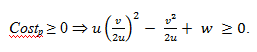
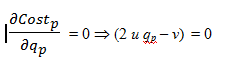
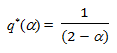
(1.5) Therefore, the parameters u ; v ; w have to meet this condition: (4 u w − v2 ) > 0. In order to minimize the total cost, the optimal value q*p can be calculated by solving this equation:

(cf. strictly positive levels of research activities).
- 2.4
- The second assumption is that the project revenues Incomesp are independent from the levels of activities qp. For each project p, Incomesp can be explained by a given amount ip of public funding under certain conditions.
For example, companies participating in projects certified by competitiveness clusters, via a consortium contract, can receive a public funding. Partners in a joint project is a consortium, which is a group of momentary separate legal entities with no legal personality, based on a purely contractual cooperation. The parties decide to pool resources for the realization of a project, and undertake to perform the services, and to share the risks and performance of this project. A budget for this project is established taking into account the personnel costs, direct and indirect costs of each party. European or national funding can be provided by each member. Each member supports the additional funding necessary to carry out its part of the project. Therefore, there are considered as constant for each project p.
Incomesp= ip where ip > 0 (2) The gross margin of a project p can be expressed by:
GMp = Incomesp - Costp
(1) and (2) ⇒ GMp = ip - u qp2 + v qp - w(3) The third and last assumption concerns the interaction between the two investment levels q1 and q2. In econometrics, a usual way to model interactions is to consider the interaction as a multiplicative term of q1 and q2 (Blackwell 1953; Topkis 1987). This can be expressed by the multiplicative expression (α q1 q2) where α is the interaction strength between q1 and q2 and -1 ≤ α ≤ +1.
- 2.5
- α > 0 is the case of complementary projects i.e. when the research activity of the project 1 rises, this leads to a rise in the activity of the project 2 and vice versa.
α < 0 is the case of substitute projects i.e. when the research activity of the project 1 rises, this leads to a fall in the activity of project 2 and vice versa. α = 0 is the case of two independent projects.
- 2.6
- The total gross margin for the two projects is: TGM(α) = GM1 + GM2 + α q1 q2
TGM(α) = [Incomes1 − Cost1] + [Incomes2 − Cost2] + α q1 q2 = (i1 - u q12 + v q1 - w) + (i2 - u q22 + v q2 - w) + α q1 q2 Let us set: k = (i1+ i2 - 2w) with k > 0 if the total revenues are always greater than the total fixed costs.
- 2.7
- The general form of the total gross margin is:
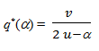
TGM(α) = vq1 + vq2 + α q1 q2 - uq12 - uq22 + k (4) The objective of the decider is to maximize TGM(α) and to find the optimal values of q1 and q2.
So the only condition where TGM is maximum is when q1= q2. This means that it is necessary to launch the same volume q* of research activities in the two complementary or substitute projects. given q2 constant ⇒ v + α q2 − 2 uq1 = 0
 given q1 constant ⇒ v + α q1 - 2uq2 = 0
⇒ (α +2u) q1 = (α +2u) q2
If α < 2u and α ≠ − 2u, then q1 = q2 ⇒ Max[TGM(α)].Then: TGM(α) = 2vq*+ α q*2 - 2uq*2 + k
And 2v + 2α q* - 4uq* = 0
- 2.8
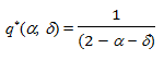
- We consider now δ as an additive misperceiving rate of the interaction strength α. We chose Siggelkow's additive assumption which corresponds to a wrong perception of α which could be expressed by (α + δ). All our simulation results have also been tested by using a multiplicative representation of the misperception: α (1 + δ) for a α ≠ 0. The behaviors of the model have been similar to the objective of this paper.
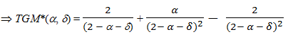
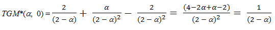
TGM*(α, δ) = Max[TGM(α, δ)] = vq1 +vq2 + α q1 q2 - uq12 - uq22 + k
Let us consider u = v = 1 and k = 0, then:
for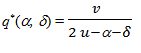
(5) 
(6) (5) and (6)
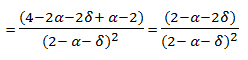
Without misperception, the total gross margin is:
Let us call loss the performance loss, loss(α, δ) = TGM*(α, δ) - TGM*(α, 0) Then:
loss(α, δ) = 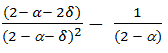
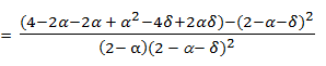
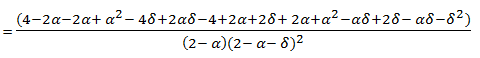
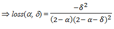
(7) This result has also been proved by Siggelkow (2002).
ABM Model formalization
- 2.9
- Agent-based models are usually defined as a set of agents who are partially autonomous and interact in a common space. No agent has a full global view of the network. We assume that there is no designated controlling agent and that the individual decisions only depend on the payoff information received from neighbors.
- 2.10
- Given :
- a set of n deciders which are distributed in a 2D square space. We assume that the edges of this space are connected to each other; the network looks like a torus.
- two complementary or substitute activities q1 and q2 in which all agents decide to invest
- an activity interaction strength parameter α
- for each agent i, a degree δi of misperception of α which corresponds to a perception (α+δ i)
- for each agent i, an expected optimal payoff function TGM*(α, δi ) for investments in optimal levels of research activities q1* and q2* which maximizes the quadratic function :
Max[TGM] = q1 + q2 +(α+δ i) q1q2 − q12 − q22 (8)
 , ri} where:
- Si = ]1,1−[ is a continuous space corresponding to each agent i to the misperception rate δi of α.
- : Si x Si' → ]1,1–[is a deterministic transition function (δi, α, δi') which describes for each agent i, the transition from a perception si = (α + δi) to s'i = (α + δi') according to the perceptions (α + δj) of all agents j (j ≠ i) who are located in the neighborhood (8, 24,… neighbors). does not depend on the past decisions (cf. homogeneous function).
- lossi: Si' → R- is the real performance loss for each agent i: lossi (α, δi') = TGM*(α, δi') − TGM*(α, 0) with TGM* the optimal payoff function (see function 7). The objective of each agent is to minimize the payoff decline lossi due to misperception.
- 2.11
- After each time period (t > 1), the real payoff TGMi is revealed to each agent i and the information transmitted by all neighbors j is TGM~j = β TGMj given an information quality rate β > 0 (0 no transmission and 1 exact information transmitted). Then, each agent i will choose a new estimation of (α +δi') according to max(TGM∼j) for j ≠ i. After this choice, he will again calculate q1i*, q2i* and TGMi* according to the new perception (α +δi').
- 2.12
- For each period t, the total performance loss is calculated by the model:
Lt = ∑i=1,…,nlossi (α, δi) (9) We developed an agent-based model for the diffusion of innovation using NetLogo environment (Wilensky 1999).
Experimental conditions
Hypothesis about the payoff function
- 2.13
- Figure 1 shows the relationship between the shortfall loss(α,δ) (function 7) and the values of the interaction strength α for different values of misperceiving δ in case of one decider and two activities. In case of complementarity (α > 0), it is better for the decision-maker to underestimate the degree of interaction (δ < 0) than overestimate it (see also Siggelkow 2002). But some situations contradict this finding (see for example in figure 1, the case where δ = +0.2 and δ = -0.5).
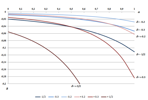
Figure 1. Shortfall loss vs complementary interaction strength α for different misperception rate δ - 2.14
- Figure 2 shows a non-linearity between loss and δ. This means that a high underestimation of the interaction strength α between two activities (δ =-1/2) is always better than a high overestimation (δ = +1/2). Nevertheless, for low overestimation or underestimation of the interaction strength α, the shortfall is also very low whatever the value of α. We finally decided in our simulations to study only two situations: α = 0.3 and 0.6.
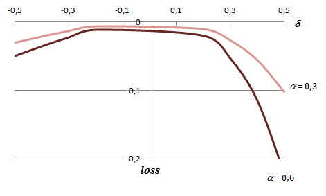
Figure 2. Shortfall loss vs misperceiving rate δ for α = 0.3 and α = 0.6 Hypothesis about the initial opinion distribution
- 2.15
- We allocated different initial values of misperception δ for each agent. For α = 0.3 and α = 0.6 and for different values of δ, we have defined a standard deviation σ which represents the dispersion of the opinion diversity. We have chosen σ so that (α +δ + 2σ) ≤ 1 if δ > 0 and (α +δ -2σ ) ≤ 1 if δ < 0 (see table 1).
Table 1: Possible scenarios for σ with different values of δ with α; = 0.3 and α = 0.6 δ = 0.3 δ = -0.5 δ = -0.3 δ = -0.2 δ = 0 δ = +0.2 δ= +0.3 δ = + 0.5 0.05 0.05 0.05 0.05 0.05 0.05 0.05 0.1 0 1 0.1 0.1 0.1 0.1 0.1 0.15 0.15 0.15 0.15 0.15 0.15 0.2 0.2 0.2 0.2 0.2 0.2 0.25 0.25 0.25 0.25 0.25 0.3 0.3 0.3 0.3 δ = 0.6 δ = -0.5 δ = -0.3 δ = -0.2 δ = 0 δ = +0.2 δ = +0.3 0.05 0.05 0.05 0.05 0.05 0.05 0.1 0.1 0.1 0.1 0.1 0.15 0.15 0.15 0.15 0.2 0.2 0.2 0.2 0.25 0.25 0.25 0.3 0.3 0.3 Hypothesis about information transmission
We considered two cases: agents share perfect information (β = 1) or the information is corrupted, badly transmitted or some agents decide to transfer wrong information (β ≠1) about their real payoff.Model validation
- 2.16
- To generate a homogeneous spatial distribution of hazards in the initial misperceiving values of δi for each agent i, the model was tested by performing 500 trials using a Monte-Carlo simulation. These initial conditions were generated by a normal distribution
 (δ, σ) with an average value of misperception δ and a standard deviation σ. Thanks to this method, different initial conditions were simulated and allowed us to identify the distribution of the global payoff values.
- 2.17
- This random assignment of δi can also partially create a segregated structure. In this case, some "islands" at the beginning of the simulation would remain and would be even stronger in some cases while others would disappear by the interplay of interactions after several iterations. In diffusion phenomena, this factor can be decisive for the spatial distribution evolution. To assess the diversity degree of this initial distribution of misperception, we calculated an entropy H based on the formula defined by Shannon (1948) in information theory:
H = - ∑i=1,…,n ∑j=1,…,m pi(j).log(pi(j)) / nlog (m) (10) with :
- n is the total number of agents
- m is the maximum number of colors. Each agent belongs to one color according to his value si =(α +δi). If we choose m = 10 different colors, each interval range is calculated according to the dispersion σ of δi and corresponds to one color.
- j is the possible "color" of each agent among m
- pi(j) is for each agent i with a color j, the proportion of neighbors including himself having the same color j over the total number of neighbor agents including himself. For example, if an agent i is "red" and among his 8 neighbors, 2 are "red", then pi(j = "red") = 1/3.
Simulation results and analysis
- 3.1
- The results are presented in four sub-sections.
- 3.2
- In §3.1, we simulated the model from t = 0 to t → ∞ (we stopped the simulation when the steady state solution was reached). We analyzed the global shortfalls at three time periods: at the beginning L0, after one period L1 and in the steady state L∞. We tried to explain the relationship between the initial diversity of opinions and L for a given decision rule defined by the function (δi, α, δ'i). Then, for different combinations of the triplet (α, δ, σ), we observed different payoff curve morphologies. We commented and tried to theoretically justify the main results.
- 3.3
- In §3.2 and §3.3, we studied the evolution of Lt considering that the information transmitted between agents concerning their individual payoff TGMi is altered by a multiplicative factor β (1 means perfect information and 0 no information transmitted). Two hypotheses were chosen: a constant initial individual factor β i for each agent i (e.g. an individual strategic behavior) and a time-varying β i (e.g. a systematic assessment error).
- 3.4
- In §3.4, we studied the influence of the neighborhood sizes on the global performance.
Behavior analysis of the global performance through time and under conditions of perfect information
- 3.5
- The first step consists in initializing the misperception rate δi of each agent i according to a given normal distribution with mean δ and standard deviation σ. Then, the first iteration computes each agent decision in parallel and can involve change in each value δi for the purpose of increasing the individual payoffs. After each period of time, a possible substitution of δi by δ'i = δj for j ≠ i and j∈
 i, the neighborhood of i, can occur if a neighbor j will transfer information about his real payoff TGM~j which can be better than TGMi. In this case, the agent i will "copy" the misperceived rate of the agent j for making his next decision.
- 3.6
- According to the scenarios proposed in table 1, we studied the evolution of the whole network shortfall Lt according to the function 9.
- 3.7
- The numeric results in Table 2 present for each couple (δ,σ) and for two cases of interaction strength rate α = 0.3 and 0.6, the different average values Lt at time t = 0, t = 1, t → ∞ and the initial entropy E0. Our 500 simulations showed a normal distribution of the results presented in table 2 with a relative confidence interval chosen as being equal to ±1.96 multiplied by the standard deviation and divided by the average value.
Table 2: L0, L1, L∞ (δ, σ) and E0 for α = 0.3 and 0.6 α =0.3 α=0.6 σ δ = - 0.5 δ = -0.3 δ = -0.2 δ = 0 δ = +0.2 δ = +0.3 δ = +0.5 δ = -0.5 δ = -0.3 δ = -0.2 δ = 0 δ = +0.2 δ = +0.3 0 L0 -31* -14 -7 0 -11 -28 -105 -51* -23 -11 0 -20 -54 L1 -31 -14 -7 0 -11 -28 -105 -51 -23 -11 0 -20 -54 L∞ -31 -14 -7 0 -11 -28 -105 -51 -23 -11 0 -20 -54 E0 - - - - - - - - - - - - - 0.05 L0 -31
±2%-14
±2-7
±3%-1
±6%-12
±2%-29
±2%-108
±1%-51
±1%-23
±2%-12
±3%-1 -22
±3%-56
±2%L1 -23
±3%-8
±3%-3
±4%0-
2%-24
±5%-50
±4%-161
±2%-39
±1%-14
±5%-4.9
±7%-3
±13%-46
±5%-93
±2%L∞ -17
±17%-4
±33%0- 0 -11
±13%-30
±19%-109
±5%-28
±13%-6
±48%0- 0- -20
±29.75%-58
±15%E0 0.2
±10%0.2
±10%0.2
±5%0.2
±30%0.2
±15%0.2
±15%0.2
±8%0.2
±15%0.2
±5%0.2
±5%0.2
±25%0.2
±10%0.2
±5%0.1 L0 -32
±2%-14
±1%-8
±4%-2
±11%-15
±6%-34
±4%-113
±3%-51
±2%-24
±3%-13
±6%-4
±3%-27
±5%- L1 -17
±2%-4
±11%-1
± 17%-8
±15%-46
±10%-85
±6%-218
±3%-29
±5%-6.9
±5%-2
±25%-15
±10%-75
±7%- L∧ -4
± 82%0- 0-
± 1%0- -12
±67%-30
±33%-119
±2%-11
±29%0- 0- 0- -21
± 51%- E0 0.5
±2%0.4
±5%0.5
±2%0.5
±4%0.4
±3%0.5
±2%0.4
± 3%0.4
±5%0.5
±4%0.5
±4%0.2
±10%0.4
±5%- 0.15 L0 -32
±3%-15
±7%-9
±3%-5 ±3% -21
±7%-42
±5%- -52
±4%-25
±1%-15
±6%-8
±4%- - L1 -11
±9%-2
±11%-2
±39%-21
±4%-78
±8%-132
±7%- -19
±10%-4
±7%-4
±28%-36
±9%- - L∞ 0- 0- 0- 0- -14
±67%-33
±33%- 0- 0- 0- 0- - - E0 0.6
±3%0.6
±2%0.6
±2%0.6
±2%0.6
±3%0.6
±3%- 0.6
±3%0.6
±5%0.6
±3%0.6
±2%- - 0.2 L0 -33
±2%-17
±7%-11
±6%-9
±7%-28
±8%-48
±6%- -52
±5%-28
±5%-19
±3%-14
±16%- - L1 -13
±9%-4
±63%-8
±19%-40
±8%-114
±8%-166
±10%- -13
±18%-7
±35%-12
±17%-47
±18%- - L∞ 0- 0- 0- 0- -13
± 80%-33
±62%- 0- 0- 0- 0- - - E0 0.7
±1%0.6
±3%0.6
±3%-0.6
±2%0.6
±5%0.6
±2%- 0.6
±2%0.7
±1%0.6 ±2% 0.6 ±3% - - 0.25 L0 -33
±4%-19
±3%-14
±8%-15
±5%-33
±8%- - -53
±4%-31
±1%-24
±4%- - - L1 -6
±23%-9
±57%-16
±34%-65
±5%-140
±2%- - -9
±20%-13
±28%-24
±19%- - - L∞ 0- 0- 0- 0- -15
±24%- - 0- 0- 0- - - - E0 0.7
±1%0.7
±1%0.7
±3%-0.7
±3%0.7
±3%- - 0.7
±1%0.7
±1%0.7
±1%- - - 0.3 L0 -34
±5%-21
±7%-18
±7%-20
±8%- - - -56
±5%-35
±6%-28
±6%- - - L1 -6
±13%-19
±33%-33
±28%-86
±16%- - - -11
±20%-20
±24%-33
±22%- - - L∞ 0- 0- 0- 0- - - - 0- 0- 0- - - - E0 0.7
±1%0.7
±3%0.7
±1%-0.7
±3%- - - 0.7
±1%0.7
±1%0.7
±1%- - - * If the confidence interval is less than 1%, we did not mentioned it in this table Total payoff evolution from L0 to L1 (first decision)>
- 3.8
- Observation 1. For all couples of misperceptions (σ ,δ), the global shortfall L1 after the first iteration is never worse (but not always better, e.g. (σ ,δ) = (0,3, -0,2)) for a small strength of activity interaction. This means that the more the activities are complementary, the more they are sensitive to misperception. The higher the degree of complementarity between two activities, the greater the consequences of the decider's misperception on the shortfall.
- 3.9
- Observation 2. For a given interaction strength α between two activities and for different values of misperceptions δ, the curve L0 (α, σ,δ) is concave ∀σ, centered on δ = 0 and is non symmetrical because underestimating seems to be better than overestimating. This first observation confirms the non-linearity between L and δ (cf. Siggelkow's function, 2002). Nevertheless, in the case of underestimation of α (cf. δ < 0), the corresponding values of L0 (α, σ ,δ) are very close whatever the value of σ. In the case of overestimation (cf. δ > 0), the dispersion of the values of L0 (α, σ ,δ) increases if δ increases. We explain this difference by the fact that in the case of underestimation of complementary activities (α > 0) if δ < 0 the shortfall function proposed by Siggelkow shows that if (α + δ ) decreases then the shortfall is very low and the differences generated by σ will not be significant.
- 3.10
- Comment. A decision-maker collects information on his neighbors' performance. When he chooses a neighbor who has a better TGM value, he knows that in fact his neighbor overestimates α (or underestimate less than himself) which implies a worse value of l. The problem is that each agent uses a payoff function maximizing TGM which is based on a wrong value of α. In fact, (α + δ) and the real payoff l which depends on the true value of α will only be revealed to them after the first period. This problem can occur when decision-makers only focus on one performance parameter and ignore its relationship with other crucial business indicators.
- 3.11
- Remark. L∞ = 0 means no global shortfall and a final state where all agent interaction perceptions match the real value of α (cf. δi = 0, ∀i).
Figure 3 shows values of L∞(δ, σ) for α = 0.3. The difference between our work and the static approach proposed by Siggelkow with one or two agents is that we seek a better understanding of the global steady-state value of L∞ according to the initial diversity of opinions between a large number of agents (this diversity is represented by σ).
Total payoff evolution from L0 to L∞
- 3.12
- We have computed the model until the total shortfall of all agents reached a stable regime. The time of simulations was initially set to infinite but the simulation runs depend on the dynamics of the computation within the model. We decided to stop the simulation at time T when the model found a stationary state minimizing LT =∑ i=1,…,n lossiT (α, δi) with n agents (we also named it L∞). Steady state corresponds to the state where all agents have a stable opinion about the value of the interaction strength between the two activities. It is interesting to note that in some cases, the final interaction strength values have not been accepted unanimously. We can also observe the emergence of some communities of agents with their own opinion about α.
- 3.13
- Observation 3. For a given interaction degree α between two activities and for different values of misperceived δ, the curves L1 and L∞ (α, σ ,δ) are concave or semi-concave ∀σ (figure 3).
- 3.14
- Another interesting result is that even if the initial total shortfall L0 has a high negative value (see table 2), the dynamics of the agent interactions sometimes allow for the reduction of the shortfall to 0.
- 3.15
- Observation 4. For a given α, if there is a high initial heterogeneity of opinions (cf. a large value of σ), it is better to underestimate α rather than to overestimate it.
- 3.16
- Observation 5. Figure 3 also shows that, if δ < 0 ∀ σ the shortfall evolution is always L0<L1<L∞ (except for δ >= 0.25) which confirms the improvement due to information sharing. If δ > 0, L∞ is also better than L1 but L0 is better than L1 (L0 > L1 and L∞> L1). This means that the transition function works better in the case of underestimation of the activities interaction strength α (after one transition and until steady state). The performance of a decider in a cooperative neighborhood continuously improves over time if she underestimates the strength of interaction between two activities. This suggests that the decision-makers' performance will be better if they are pessimistic and cooperative.
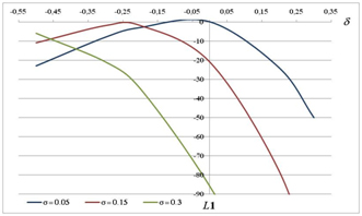
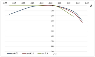
Figure 3. Shortfalls L1 and L∞ vs misperception level δ and dispersion rate σ ( for α = 0.3) - 3.17
- Managerial impacts: Our main question was to find a relationship between the initial opinion diversity σ of each agent which is represented by δi = (δ ,σ) (the "general" opinion is supposed to be the mean value δ) and the final total payoff (cf. the total shortfall L∞ to minimize) when the steady-state value has been reached. This question is very suitable for a high-tech innovative cluster launching two new complementary projects. After choosing a level of investments in these projects, we assumed that each decider transfers his payoff information to his neighborhood after each period of time (for instance every six months). Our results show that the transition between the first global payoff of the network at t = 0 and the second one at t = 1, highly depends on the initial opinion diversity but this becomes false after a long period. In the case of overestimating the interaction strength, a temporary shortfall reduction could lead the deciders to stop their cooperation and thus, stop their individual investments in the project. Such a decision may stop the diffusion of interesting ideas in terms of achieving technology-intensive projects like in competitiveness clusters. Our model does not recommend such a myopic and short term view which focuses on immediate financial results. It shows a possible improvement of the long-term performance even if the initial agent opinions are highly diverse.
Total payoff evolution of Lt(α, δ, σ)
- 3.18
- Figure 4 shows the evolution of Lt for the following scenarios:
- two complementary activities with an interaction strength α = 0.3 (We also simulated the case of α = 0.6 which provided similar results)
- two different misperception degrees of δ : α = -0.2 (underestimation); δ = +0.2 (overestimation)
- three dispersions of the initial agent opinions σ = 0.05 ; σ = 0.1; σ = 0.25
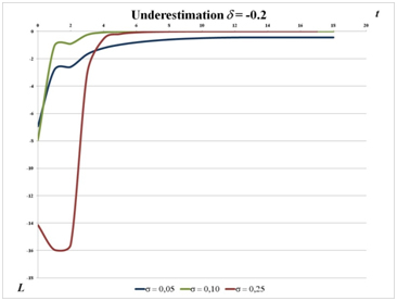
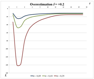
Figure 4. Lt for different values of σ with δ = -0.2 (underestimation of α = 0.3) and δ = 0.2 (overestimation of α) - 3.19
- Observation 6. In case of the underestimation of α (left side of figure 4), if the initial opinion σ is low, the total payoff improves with time due to information sharing. Nevertheless, if σ is high (for instance 0.25) or in the case of overestimation (right side of figure 4), we observe another curve morphology: if the dispersion of opinions σ increases, the gap between L0 and Lmin increases although the steady state shortfall LT will be very low ∀σ. In the case of a large number of companies working on two projects with high technology (e.g. observation 2), a large range of opinions can exist during the project launching. This diversity of opinion may affect the first decision making process and lead to bad choices. This can be explained by the fact that some managers have chosen to trust the wrong person in their neighborhood. Nevertheless, in case of decisions being taken on a recurring basis, all managers tend to homogenize their opinions. A high level of heterogeneity can lead to a delay in performance improvement.
- 3.20
- Theoretical justification. If σ >> 0 and δ > 0, then L0 >> L1 (table 2 and figure 4). The reason is that each agent i who selects a neighbor j such as max(TGMj) > TGMi ∀ j≠ i, knows in fact that j overestimates α which implies a worse value of loss (cf. function 7, figures 1 and 2) and of L. After this first choice, the real payoff value TGM∼ is revealed and TGM∼ is always lower than TGM if δi > 0 (overestimation of α) because TGM∼ only depends on α and TGM on (α + δi). These real values TGM~ will be shared within the network. At the next decision, all values will be therefore reduced and consequently L will increase. This justification is valid for an overestimation of α (δ > 0) but also in the case of underestimation with high initial opinion diversity. In this last case, the normal fluctuations of δ = -0.2 (cf. underestimation) with σ = 0.25 generate values of δi which can be positive, and therefore amount to an overestimation of α.
- 3.21
- Observation 7. In the previous figure 4, we can observe two different shortfall curve morphologies:
- Payoff curve morphology PCM1: in the beginning of the simulation Lt looks like a non-monotone convex function and will after this launching period exponentially increase to finally become asymptotically stable (see on the left side of figure 4 when σ = 0.25 and &8704;σ on the right side). In the early stages, the overall performance of each decider falls to a minimum, then rises rapidly and stabilizes at a value close to 0. In this case, the decision-makers have reached a perception degree of the project interaction which is close to reality.
- Payoff curve morphology PCM2: Lt exponentially increases very rapidly at first, and then levels off to become asymptotic to an upper limit (see figure 4 left when σ ≤ 0.15). In this case, the decision-maker's overall performance improves rapidly to reach a stable state which corresponds to a consensus about the interaction strength between the two projects. This interaction perception is not necessarily the real value.
- 3.22
- Theoretical justification. These results depend on the initial diversity of opinion and on the decider's decision rules. To attempt to explain the emergence of these curve morphologies, we will divide the network into three populations of agents that we have called winners, losers and neutrals. Their individual size evolves according to the decision rules launched at each period of time (the sum of the three population sizes remains equal to the whole population size). The rules are the following: at time t = 1, each agent i chooses the couple (α , δj) of the neighbor j who has the best payoff TGMj. From t = 2 to T (at steady-state), the real payoff TGM~i is revealed to each agent. Then, he chooses a new estimation of α according to the best perceived value TGM~j of one of his neighbors.
- Characteristic of the loser population evolution. The losers are agents who see their real payoff fall: TGMt+1 < TGMt. Losers can only appear from time t = 2. Losers are deciders who make a choice which leads to a performance decrease.
- Characteristic of the winner population evolution. At time t, winners improve their payoff so as: TGMt+1 > TGMt. Winners are deciders who make a choice which leads to a performance increase.
- Characteristic of the neutral population evolution. Neutrals are agents who cannot find a best payoff TGM in their neighborhood and therefore do not change their minds TGMt+1=TGMt. Neutrals are deciders who don't change their opinion.
- 3.23
- Our theoretical justification is based on four cases:
- Case 1: underestimation of the interaction α between two complementary activities with a high initial opinion diversity σ (with payoff curve morphology PCM 1)
- Case 2: underestimation of α with a low initial opinion diversity σ (with PCM2)
- Case 3: overestimation of α with a high initial opinion diversity σ (with PCM1)
- Case 4: overestimation of α with a low initial opinion diversity σ < 0.15 (with PCM 1)
Case 1
- 3.24
- Figure 5 shows the evolution of the real payoff TGMi(t) of each agent i. Due to information sharing, we can see a homogenization of TGMi towards a constant value (i.e. a same misperception of interaction strength α) after a given period of time T= 19.
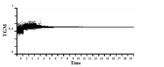
Figure 5. Distribution of payoffs TGM for the 1024 agents from t =0 to T = 19 - 3.25
- Despite a high dispersion of the individual misperceptions δi at t = 0 and t = 1 (cf. the values of TGMi), the model finally converges towards a same opinion (see figure 6, the light red islands at t = 1 become the dominant color at t = T).
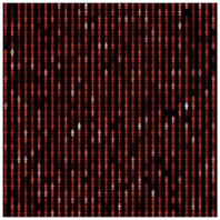
t = 0 t = 1 T = 19 Figure 6. Spatial repartition of the misperception of each agent - 3.26
- These observations can be particularly explained by the evolution of the neutral population (figure 7). Because of a high initial opinion heterogeneity, the first choice made by the agents does not allow for an apt homogenization of the opinions and hence avoid the emergence of losers. In fact, the number of losers rapidly grows, reaches a maximum and then decreases.
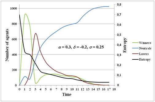
Figure 7. Winners, losers, neutrals and entropy evolutions (underestimation of α with a high initial opinion diversity σ) - 3.27
- At the beginning, the entropy is high (almost 0.70) and rapidly decreases, slows and tends toward zero at t = 14. These three periods of decline can be explained by a relatively strong reduction in the first period until t = 2 which corresponds to the winner peak and the increase of the number of losers. Then a slower second period follows with a decline in the number of winners until it becomes equal to the number of losers. This second period is justified by the transition rule. At t = 2, the agents perceive the real value and choose in their neighborhood the agent with the highest perceived payoff TGM~j. The third period corresponds to a slow decay of the entropy coinciding with the transfer of winners and losers towards neutral agents whose population increases (principle of communicating vessels). At t = 3, the number of winners increases, then declines and is followed at t = 9 by a reduction of the number of losers. This phenomenon has, as a consequence, a continuous increase of the neutral population (but less strong). At t = 12, a simultaneous decrease in the number of winners and losers increases the amplitude of the neutral evolution which decreases progressively when the winner and loser population disappears. These explanations justify the curious evolution Lt (cf. PCM 1) which shows that it is possible to improve the total payoff even if the initial payoff is low.
Case 2
- 3.28
- In this case, Lt follows a curve morphology PCM2 which can be explained by the fact that for a low initial opinion dispersion, there are no losers, so the global shortfall Lt will not decrease (figure 8). More generally, if σ = 0+ (cf. opinions of each agent on δ are very close), the heterogeneity is considerably reduced after one period of time (t = 1). At t = 1, the number of winners sharply grows after decreasing. Without losers and given that the total number of agents is constant, reducing the number of winners increases the neutral agent population (they do not find an agent in their neighborhood with a better payoff value TGMj). At the beginning, entropy is relatively low (almost 0.20) and decreases rapidly until zero at t = 5. This reduction occurs in two periods: a relatively slow first period until t = 2 which corresponds to the peak in winners, then a much stronger second period followed by the decline in winners. This second period can also been explained by the transition rule.
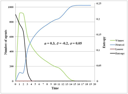
Figure 8. Winners, losers, neutrals and entropy evolutions (underestimation of α with a low initial opinion diversity σ) Cases 3 and 4
- 3.29
- We observe the same evolution that was present in the first case with a high initial opinion diversity (underestimation of α = 0.3 with δ = -0.2 and σ = 0.25) in correspondence with the left side of figure 4 and PCM1. This means that the final shortfall LT tends towards zero even if the initial activities interaction is very high. Eventually, all the decision-makers find an interaction strength value that is close to the real value.
Impact of strategic information distortion (Hypothesis 1) on global performance
- 3.30
- It is well known that cooperation and information sharing are the key variables of innovation policies but there is often an information distortion between the transmitter and the receiver during transmission and/or collection in the communication channel. This distortion is sometimes intentionally chosen by the decider for various strategic reasons. For example, the decision-maker thinks he has obtained a competitive advantage and does not wish to reveal some results. The distortion can also be unintentional and the information transmitted inaccurate.
- 3.31
- An information transmission distortion is considered as being normally distributed among the agents with a quality rate β i > 0. We initialized β i using a normal distribution with mean 1 (perfect quality of transmission) and a standard deviation ξ (we truncate the distribution in case of β i < 0).
- 3.32
- The first hypothesis H1 considered that each agent i chooses an initial value β i which corresponds to his individual choice of communicating wrong information to his neighbors. He decides initially to communicate a higher ( β > 1) or a lower ( β < 1) payoff value TGM∼ = β TGM than his actual value TGM. He will not change his strategy over time, therefore β i remains constant (a second hypothesis is presented in §3.3). We have not considered that agent i can learn about his neighbor strategies and improve his understanding of β i after each decision.
- 3.33
- To study the impact of the information quality of the global performance, we have considered two cases where the initial opinions on α are extremely different or very close. In the first case, each agent initially has his own opinion. In the second case, we studied only the real impact of the quality of information transmission on the total payoff but we had to choose σ = 0+ to generate a small initial diversity of the agents. If firms don't know anything about α, the competitiveness cluster governance can inform the investors' that two complementary projects have an expected perception δ of the interaction strength α. Once this information is transferred, after the first period of time, the deciders will partially share information about their payoffs in order to improve their understanding of α.
- 3.34
- In order to facilitate comparison of results with those of the previous section §3.1( β = 1), we used the same case numbering (see table 3).
Table 3: Simulation scenarios in cases of underestimation vs overestimation of an activity interaction α = 0.3 Information quality δ σ Case 1 (1,ξ = 0.05) and (1,ξ = 0.25)-0.2 (underestimation) 0.25 Case 2 (1,ξ = 0.05) and (1,ξ = 0.25)-0.2 (underestimation) 0.05 Case 3 (1,ξ = 0.05) and (1,ξ = 0.25)+0.2 (overestimation) 0.25 Case 4 (1,ξ = 0.05) and (1,ξ = 0.25)+0.2 (overestimation) 0.05 - 3.35
- Observation 8. Figure 9 shows a steady state at T= 9 and the overall payoff curve morphology looks like PCM1. An original result confirms that in the case of overestimation of interaction strength α and imperfect information (ξ > 0), the global shortfall LT does not improve as much as in the case of perfect information (1, 0) (figure 4).
- 3.36
- Observation 9. In the case of underestimation and whatever the range of the information quality rate (∀ ξ > 0), the global shortfall LT is always very close but is worse than in the case of perfect information (1, 0).
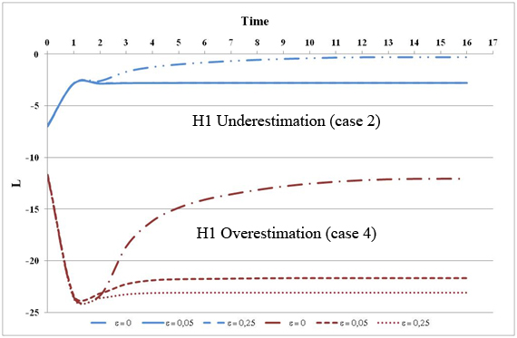
Figure 9. Lt for different values of ξ with σ = 0+ and δ = -0.2 (underestimation of α = 0.3) and δ = +0.2 (overestimation of α) Observation 10. The global shortfall LT in the case of high diversity of opinion (figure 10) is worse than in the case of low initial diversity with perfect (figure 4) or imperfect information (figure 9).
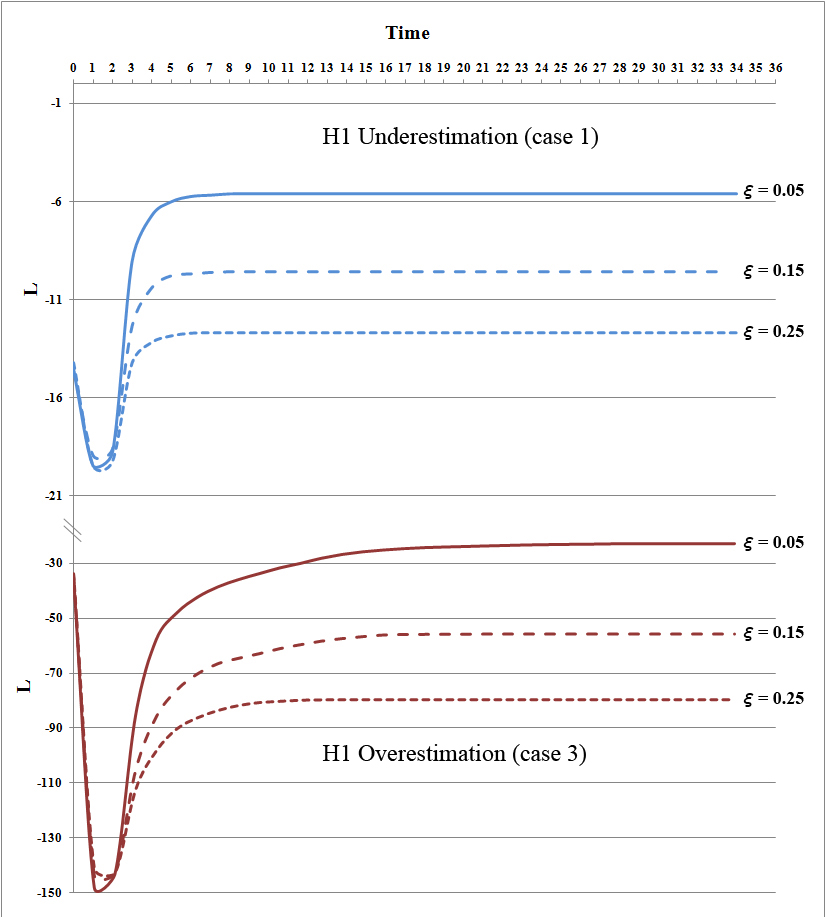
Figure 10. Lt for different values of ξ with σ = 0.25 and δ = -0.2 (underestimation of α = 0.3) and δ = +0.2 (overestimation of α) - 3.37
- Observation 11. Despite an expected final stability LT reaching a fixed point, we have detected a high heterogeneity of the final agent opinions. Figure 11 shows the differences between the agent real payoffs TGMi (cf. their different opinions about α at t = T) whatever (i.) the initial opinion diversity (∀ σ > 0), (ii.) the initial dispersion of the agent quality information (∀ ξ > 0) and (iii.) the type of misperception of α (under vs overestimation, ∀ δ ≠ 0).
- 3.38
- Comment. This observation explains why the overall payoff LT is insufficient (see observation 10 above). We proved that the information sharing hypothesis H1 deteriorates the total payoff because agents are less cooperative. The only change to the reference model was the addition of the parameter ξ.
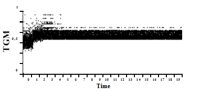
Figure 11. Heterogeneity of the individual opinions (TGMi between t =0 and T = 19) 
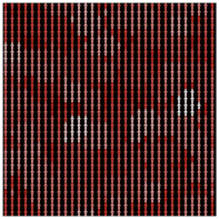
Figure 12. Steady-state opinions pattern - 3.39
- Observation 12. We also found a clustering phenomenon (Figure 12). The number of clusters is equal to the number of possible stable values of TGMi (figure 11 at T=19) and the agent colors are calculated according to the parameter (σ + δi), which matches the payoff values TGMi.
Impact of assessment errors (Hypothesis 2) on global performance
- 3.40
- We assume that investors are having difficulties in evaluating their real payoff and communicating to the neighbors an inaccurate value. The estimation error is normally distributed with mean 0 and standard deviation ξ. Therefore, the information quality factor β i is generated at each period by a normal distribution (1, ξ).
- 3.41
- The simulations were based on the same scenarios as shown in §3.2 Table 3.
- 3.42
- Observation 13. Figure 13 shows a steady state which means that even if the information quality fluctuates over time, the model tends to stabilize at LT after a long period T = 300. In the case of overestimation of α, the global shortfall LT is always better or equal to all other previous cases (Figures 4 and 9). This means that it is better that information fluctuates over time (cf. H2) rather than only at the beginning (cf. H1). We observed the same behavior in the case of high initial opinion diversity (σ = 0.25).
- 3.43
- Theoretical justification. In this H2 scenario, the difference is explained by the fact that the model reaches a homogeneous opinion pattern contrary to H1 (figures 11 and 12).
- 3.44
- Observation 14. The time to achieve the steady state performance (H1) is ten times (for ξ = 0.05) or thirty times (for ξ = 0.25) longer than was previously the case (H2).
- 3.45
- Comment. It should be interesting to compare the cumulative shortfall ∑t=0,…,T Lt for H1 and H2 and to observe the intersection from which H1 becomes better than H2.
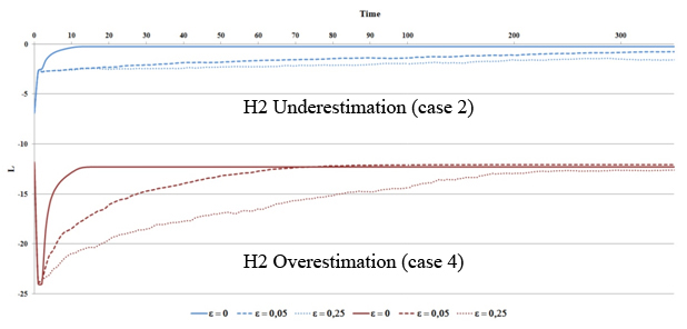
Figure 13. Lt for different values of ξ with σ = 0+ and δ = -0.2 (underestimation of α = 0.3) and δ = +0.2 (overestimation of α) Effect of the neighborhood size
- 3.46
- Instead of considering information sharing in a Moore neighborhood, we have expanded the influence area of each agent to 24, 48 and 80 neighbors. It should be noted that our model is composed of 1024 agents distributed in a 2D square space but the edges are connected to each other (it looks like a torus).
- 3.47
- Observation 16. The larger the influence area of each agent is, the higher the total payoff loss is regardless of the scenario of information sharing quality (table 4).
- 3.48
- Theoretical justification. Based on observation 6 in §3.1 which has been justified, the probability that each agent i selects a neighbor j such as: max(TGMj) > TGMi, ∀ j ≠ i, grows according to the size S of the neighborhood. This implies a greater probability to choose a neighbor j who overestimates α and provides a worse value of loss (cf. function 7). The more S is large, the more the opinion diffusion increases. This is explained by the high number of neighbors which very quickly stabilizes the global opinions (cf. reaching rapidly a fixed point with opinion convergence) while avoiding an increased improvement to the total payoff.
- 3.49
- Observation 16. The more neighbors there are, the less sensitive the model is to information quality ξ.
- 3.50
- Observation 17. If ξ increases, then the global shortfall LT is better in the case of H2 than H1. This can be explained by the type of distortion βi of the information transmitted by each agent. For H1 this factor is constant in time and is variable for H2. This gives more possibilities in the case of H2 to achieve a better fixed point.
Table 4: L∞ (δ, σ, ξ) for α = 0.3 and for different sizes S of neighborhood Case 1
(underestimation of α)S = 8 S = 24 S = 48 S = 80 Case 3
(overestimation of α)S = 8 S = 24 S = 48 S = 80 H1
(σ= 0.25)ξ=0 0- 0- -7 -34 H1
(σ= 0.25)-10 -77 -144 -215 ξ=0.05 -5.6 -10 -22 -31 -22.7 -78 -148 -177 ξ=0.15 -9.6 -17 -32 -34 -56 -101 -147 -184 ξ=0.25 -12.7 -20 -40 -40 -79.5 -80 -188 -214 H2
(σ= 0.25)ξ=0 0- 0- -7 -34 H2
(σ= 0.25)-10 -77 -144 -215 ξ=0.05 -0.09 -1 -14 -27.5 -13.8 -77 -139 -182 ξ=0.15 -0.1 -3.5 -13.6 -33.7 -9 -77 -135 -190 ξ=0.25 -0.3 -2.4 -14.6 -32.8 -20 -70 -145 -161
Synthesis and research outlooks
- 4.1
- Few studies have shown that misperception of the interaction strength between activities limits global performance (Siggelkow 2002). To our knowledge, no research has paid attention to the situation where a large number of agents shared information in a same space (e.g. an innovative cluster). This paper considers managers who share their payoff information in order to improve their understanding of the interaction strength α between two complementary activities in which they choose to periodically invest (It should be remembered that we only choose to work on complements because many authors have shown that misperception had little influence on the shortfall in case of substitutes). They communicate with their close neighbors to better estimate α in order to reduce their shortfall. We also assumed a possible distortion of the quality of the shared information. This is due to neighbors transmitting wrong information about their payoff based on two hypotheses: H1, each manager does not change his initial strategy and disseminates inaccurate information over time and H2, unintentional information fluctuations due to assessment errors at each decision.
- 4.2
- Such situations could appear in competitiveness clusters where firms invest time after time in two complementary projects. Our model advises to avoid a myopic and short term view that focuses on immediate financial results, and shows a possible improvement of the long-term performance even if the initial agent opinions about α are very diverse and/or the information quality is low.
Main results
- 4.3
- Our model studies the dynamic evolution of an agent-based model composed by decision makers who try to reduce their misperception of the interaction of two projects. The first observations show, from an economic point of view, that it is generally better to underestimate the interactions of activities than to overestimate (see also Siggelkow's results 2002). Qualitatively speaking, managers' opinions usually converge after reaching a steady state. This is not the case for the hypothesis H2 where opinions remain different for a lot of managers (but stable) after reaching a steady state. This means that if inaccurate information is changing at each decision, the individual decision rule based on information sharing is not able to standardize the managers' opinions and therefore can't improve the global steady state performance enough. Another result shows, especially in the case of high initial opinion divergence (cf. a high dispersion of initial misperceptions), that the total shortfall L of the network after launching two new projects in which managers cannot accurately estimate the interaction strength α, declines very rapidly.
- 4.4
- We also found a counterintuitive result which shows that if each agent increases his neighborhood influence size, the final performance will decline.
Research outlooks
Empirical validation
- 4.5
- We will test our model on innovative companies that cooperate together with imperfect information within competitiveness clusters. We will focus on firms working simultaneously on two R&D projects funded by the contractor. The investment choices are based on these given grants and on a U-shaped cost function. This is particularly the case for companies working at the same time in two clusters on different projects. We already know innovative firms working simultaneously on two projects within the cluster Sysolia (industrial solar systems) and on projects funded by the cluster Route des Lasers (development and dissemination of innovative technologies of optics and lasers - laser systems and applications, metrology, imaging, physics innovative - in industry). This future work will be implemented during these project lifecycles. Nevertheless, relevant information may appear when we compare the field results in a real neighborhood with those provided by our model. However, an additional problem may arise. Indeed, some innovative companies in high-tech areas are reluctant to provide financial information that are confidential for them. It is a study that requires patience based on mutual trust.
- 4.6
- In our model (of competitiveness clusters, we wish to represent different types of agents (universities, SMEs, large companies, technology platforms, etc.), each with different objective functions (volume of publications, ROI, etc.). Furthermore, the addition of different cooperation strategies according to each agent's type can be simulated and their impact on performance can be studied on an individual scale, on the scale of a group of agent's and of the overall cluster. We could also consider the adaptive behavior of the agents and identify its implications which can be similar to a supermodular game (Milgrom and Roberts 1990). More complex decision-making behavior, learning and memory as well as information channel diversification and objective functions could be also incorporated into the model in reference to some empirical works of authors (Younès 2011) and your own future empirical studies.
Model extensions
- 4.7
- We postulated that the opinion diversity was a randomly generated initial state according to a Gaussian distribution. We justified this method by the fact that deciders have to launch new activities and therefore don't have a close opinion of the interaction strength between the two projects. One extension could be to integrate into the model the knowledge provided by some managers who have had past experiences on similar activities. These managers could transmit their knowledge to other managers. For example, in some competitiveness clusters, there are training platforms where firm employees and managers can be trained on topics related to the cluster's themes. This would avoid the sharp performance decrease observed after the first decision.
- 4.8
- Another extension regarding the hypothesis H2, will consist in considering the risks of a long waiting period to reach stable opinions and to minimize losses for the whole network. This period may lead some deciders to stop their funding due to a too high cumulative shortfall. The gradual disappearance of agents could have an impact on the overall system behavior. For example, in the competitiveness cluster, some firms stop their collaborations in projects.
- 4.9
- We considered in our model the agent's space as a torus. It is possible to transform this space in a bounded square, which would limit the number of neighbors in the edges. Finally, the choice of metric in a cluster context for example also remains to be studied. Beyond the Euclidean distance, other dimensions could be taken into account (e.g. social distances)
- 4.10
- Finally, we wish to complete the model by expanding the rules of inter-individual perception taking into account confidence and belief. Some research has incorporated these elements in multi-agent models (Thiriot and Kant 2008) as well as knowledge sharing (Wang et al. 2009) or information transmitted by word of mouth (Thiriot and Kant 2010). This work, often applied to marketing, has limitations however due to the complexity of social interactions and individual behavior.
Acknowledgements
-
We gratefully thank the reviewers for their constructive comments and suggestions. We also acknowledge the manager of Alphanov, the technological platform of Bordeaux innovative cluster Route des lasers, for giving us the opportunity to share our ongoing research.
Notes
References
-
BLACKWELL, D. (1953). Equivalent Comparison of Experiments. Annals of Mathematics and Statistics, 24(2), 265–272. [doi:10.1214/aoms/1177729032]
GALBRAITH, J. R. (1977). Organization Design. Reading, Massachusetts : Addison-Wesley.
GUISO, L. & Schivardi, F. (2007). Spillovers in industrial districts. Economic Journal, 117, 68–93.
KHANDWALLA, P. N. (1973). Viable and effective organizational designs of firms. Academic Management Journal. 16, 481–495. [doi:10.2307/255008]
MILGROM, P. & Roberts, J. (1990). Rationalizability, Learning, and Equilibrium in Games with Strategic Complementarities. Econometrica, 58 (6), 1255–1277. [doi:10.2307/2938316]
MILLER, D. & Friesen, P. H. (1984). Organizations: A Quantum View. Englewood Cliffs, NJ : Prentice Hall
PORTER, M. E. (1996). What is strategy?. Harvard Business Review, 7, 4(6), 61–78.
PORTER, M. E. (2007). Clusters and Economic Policy : Aligning Public Policy with the New Economics of Competition. Harvard Business School ISC White Paper, Rev. 10/27/09
SHANNON, C.E. (1948). A Mathematical Theory of Communication. The Bell System Technical Journal, 27, 379–423, 623–656. [doi:10.1002/j.1538-7305.1948.tb00917.x]
SIGGELKOW, N. (2002). Misperceiving Interactions among Complements and Substitutes: Organizational Consequences. Management Science, 48(7), 900–916. [doi:10.1287/mnsc.48.7.900.2820]
THIRIOT, S. & Kant, J. D. (2008). Using associative networks to represent adopters' beliefs in a multi-agent model of innovation diffusion. Advances in Complex Systems, 11(2), 261–272.
THIRIOT, S., & Kant J. D. (2010). A naturalistic multi-agent model of word-of mouth dynamics. In K. Takadama, C. C. Revilla, G. Deffuant (Eds.), Simulating Interacting Agents and Social Phenomena, The Second World Congress on Social Simulation, Agent-Based Social System Series (pp. 89–99), Springer Japan. [doi:10.1007/978-4-431-99781-8_7]
TOPKIS, D.M. (1987). Activity optimization games with complementarity. European Journal of Operational Research, 28(3), 358–368. [doi:10.1016/S0377-2217(87)80179-0]
WANG, J., Gwebu, K., Shanker, M., & Troutt, M. D. (2009). An application of agent-based simulation to knowledge sharing. Decision Support Systems, 46(2), 532–541. [doi:10.1016/j.dss.2008.09.006]
WILENSKY, U. (1999). NetLogo. Center for Connected Learning and Computer-Based Modeling, Northwestern University, Evanston, IL. http://ccl.northwestern.edu/netlogo/.
YOUNES, D. (2011) Creating cooperation ? : the partnering dynamics in Saclay's competitiveness cluster, Unpublished Diploma thesis: Science Po, Paris.
Source pseudo code
-
Function setup
Create the number of agents
For each agent
Move the agent in his own area (one agent by area)
Assign value to deltarandom (normal distribution with a null average value and a standard deviation assigned by the user)
Assign value to delta (deltainitial + deltarandom)
Assign value to betarandom (normal distribution with a null average value and a standard deviation assigned by the user)
Assign value to beta (betainitial + betarandom)
While beta < 0
Assign value to betarandom (normal distribution with a null average value and a standard deviation assigned by the user)
Assign value to beta (betainitial + betarandom)
End
Assign value of α's perception by each agent alphadelta (alpha + delta)
While alphadelta < -1 or alphadelta > 1
Assign value to deltarandom (normal distribution with a null average value and a standard deviation assigned by the user)
Assign value to delta (deltainitial + deltarandom)
Assign value to alphadelta (alpha + delta)
End
Assign a color to each agent between -1 and 1 and proportional of his own value of α's perception
End
For each agent simultaneously
Assign value to q1 (1 / (2 - alphadelta) )
Assign value to q2 (q1)
Assign a value to TGM (q1 + q2 + ((alphadelta) * q1 * q2) - (q1 ^ 2) - (q2 ^ 2))
Display individual value of TGM
End
For each agent simultaneously
Assign the last value known of TGM in a short memory variable OldTGM (TGM)
Choice of the value of alphadelta of the neighbor having the best value of TGM
Assign a new value to TGM by using the new value of alphadelta
If oldTGM < TGM then
Assign the value 1 to the agent variable winner
Assign the value TGM to the agent variable TGMwinner
End
If oldTGM > TGM then
Assign the value 1 to the agent variable loser
Assign the value TGM to the agent variable TGMloser
End
If oldTGM = TGM then
Assign the value 1 to the agent variable loser
Assign the value TGM to the agent variable TGMneutral
End
Assign a new color to the agent by using the new value of alphadelta
Display the new individual value of TGM
Display the number of winners, losers and neutrals
End
End
Function go
Repeat
Function neighbors
Increment the counter
Until stop
End
Function neighbors
For each agent simultaneously
Assign 0 to winner
Assign 0 to loser
Assign 0 to neutral
Assign 0 to TGMwinner
Assign 0 to TGMloser
Assign 0 to TGMneutral
Assign the last value known of TGM in a short memory variable OldTGM (TGM)
Assign a value to real TGM by using the value of α TGMreal(TGM + TGM + ((alpha) * TGM * TGM) - (TGM ^ 2) - (TGM ^ 2))
Assign a value to perceived TGM (beta * TGMreal)
Choice of the value of alphadelta of the neighbor having the best value of the perceived TGM
Assign a new value to q1 (1 / (2 - alphadelta) )
Assign a new value to q2 (q1)
Assign a new value to TGM with the new value of q1, q2 and alphadelta (q1 + q2 + ((alphadelta) * q1 * q2) - (q1 ^ 2) - (q2 ^ 2))
If oldTGM < TGM then
Assign the value 1 to the agent variable winner
Assign the value TGM to the agent variable TGMwinner
End
If oldTGM > TGM then
Assign the value 1 to the agent variable loser
Assign the value TGM to the agent variable TGMloser
End
If oldTGM = TGM then
Assign the value 1 to the agent variable loser
Assign the value TGM to the agent variable TGMneutral
End
If the option of calculating beta in each time is selected then
Assign a new value to betarandom (normal distribution with a null average value and a standard deviation assigned by the user)
Assign a new value to beta (betainitial + betarandom)
While beta < 0
Assign a new value to betarandom (normal distribution with a null average value and a standard deviation assigned by the user)
Assign a new value to beta (betainitial + betarandom)
End
End
Assign a new color to the agent in using the new value of alphadelta
Display the new individual value of TGM
End
Assign to TWinner the sum of winners
Assign to TLoser the sum of losers
Assign to TNeutral the sum of neutrals
Assign to TotalTGMWinner the sum of TGM of winners
Assign to TotalTGMLoser the sum of TGM of losers
Assign to TotalTGMNeutral the sum of TGM of neutrals
Assign to TL the sum of l of all agents (sum [(- (alphadelta - alpha) * (alphadelta - alpha)) / ((2 - alphadelta) * (2 - alphadelta) * ( 2 - alpha ))] of agents )
Display the number of winner, loser and neutral
Display TL
End