
 Abstract
- We address theoretically whether and under what conditions Schelling's celebrated result of 'self-organized' unintended residential segregation may also apply to school segregation. We propose here a computational model of school segregation that is aligned with a corresponding Schelling-type model of residential segregation. To adapt the model for application to school segregation, we move beyond previous work by combining two preference arguments in modeling parents' school choice, preferences for the ethnic composition of a school and preferences for minimizing the travelling distance to the school. In a set of computational experiments we assessed the effects of population composition and distance preferences in the school model. We found that a preference for nearby schools can suppress the trend towards self-organized segregation obtained in a baseline condition where parents were indifferent towards distance. We then investigated the joint effects of the variation of agents' 'tolerance' for out-group members and distance preference. We found that integrated distributions were preserved under a much broader range of conditions than in the absence of a preference for nearby schools. We conclude that parents' preferences for nearby schools may be an important factor in tempering for school choice the segregation dynamics known from models of residential segregation.
- Keywords:
- Schelling Model, Ethnic Segregation, School Segregation, Model Alignment
Introduction
- 1.1
- Schelling's model of residential segregation (Schelling 1969, 1971, 1978) shows that the high level of ethnic (or, racial, in the American terminology) residential segregation observed in many modern cities can be an unintended outcome of the residential choices of individuals who have only the "mild" ethnic preference to not be outnumbered too much by other ethnic groups in their local residential neighborhood. However, Schelling's result has hardly influenced the study of other social segregation phenomena, most notably not in the debated field of school segregation (e.g. Sohoni and Saporito 2009; Van Houtte and Stevens 2009; Logan et al. 2008). We make a first step to advance existing work based on Schelling into the field of school segregation and to explore similarities and differences between residential and school segregation dynamics with an alignment (Axtell et al. 1996; Rouchier et al. 2008) of simple theoretical models of both phenomena.
- 1.2
- In Schelling's model, integrated residential distributions are typically unstable, even when individuals are largely tolerant of other ethnic groups in their neighborhood, but prefer not to belong to too small a minority. If residents of a small local minority leave a neighborhood, this changes the local ethnic mix such that members of their ethnic group become even more likely to leave, which eventually pushes the residential distribution away from instable integration towards stable segregation. This self-reinforcing "preference dynamics" (Clark and Fossett 2008) can generate much more segregation than would be needed to satisfy individuals' ethnic preferences, an undesired outcome from the individuals' perspective, with potentially severe negative societal consequences. Similar preference dynamics may underlie the high level of ethnic school segregation that can be found in many Western countries nowadays (Logan et al. 2008; Baker et al. 2011).
- 1.3
- School segregation refers to the disproportionate concentration of ethnic minorities in certain schools and is a scientifically as well as politically contested topic (Sohoni and Saporito 2009; Van Houtte and Stevens 2009; Logan et al. 2008; Bovens and Trappenburg 2006; Karsten et al. 2006; Karsten et al. 2003; Saporito 2003). For example, in 2006, about 50% of primary schools in the 4 biggest Dutch cities were considered "black schools", having more than 50% non-western ethnic minority pupils, a proportion that far exceeded the national average of 14% (CBS 2007). In particular, studies of school-choice dynamics point to the phenomenon of "white flight" as a possible cause. Both for the U.S. (e.g. Logan et al. 2008; Sohoni and Saporito 2009) as well as for Western-European countries (Kristen 2008; Karsten et al. 2006), the evidence suggests that parents of the dominant ethnic group tend to choose schools outside of the local neighborhoods with relatively high concentrations of ethnic minorities. Researchers and politicians alike are concerned about the negative societal consequences of school segregation for inequality and integration of minorities (e.g.Karsten et al. 2006; Moody 2001).
- 1.4
- Empirical research on parents' school-choice motives suggests a potential for preference dynamics. A survey study for the Netherlands (Karsten et al. 2003) found that one of the most important choice motives for native Dutch parents is whether the school comprises children with the same cultural background "as us" (see also Coenders et al. 2004). If parents were to choose schools solely based on such preferences, preference dynamics might ensue which could explain the high levels of school segregation observed in Dutch primary schools. However, theories of preference dynamics in residential segregation cannot be readily generalized to school segregation. Given the strong residential segregation in Western countries, schools would be segregated even without preference dynamics, if school-choosers primarily minimize distance between home and school. In fact studies of micro-level school-choice motives revealed that parents deem both ethnic composition and distance important (Bell 2009; Denessen et al. 2005; Kristen 2008; Karsten et al. 2006; Karsten et al. 2003; Coenders et al. 2004; Saporito 2003). Parents' preference for nearby schools may even curb self-organized segregation because it discourages "flight" to more distant but ethnically more desirable schools. But whether that actually happens depends on a complex interplay of parents' choice behavior with the residential composition of their own and neighboring neighborhoods, as well as the capacity, geographical locations and current composition of available schools.
- 1.5
- The complexities of school-choice dynamics cannot simply be addressed within existing models of preference dynamics in residential segregation (e.g. Clark and Fossett 2008; Fossett 2006a; Grauwin et al. 2009; Hatna and Benenson 2012; Macy and van de Rijt 2006; Stauffer and Solomon 2007; Vinkovic and Kirman 2006; Zhang 2004a, 2004b). When it comes to school-choice dynamics, we need to distinguish between the residential location of a household which defines the distances to available schools as well as the ethnic composition of the residential neighborhood, and the ethnic composition of the schools that children from this household attend. Schools may recruit their membership from the local and surrounding local neighborhoods, but when parents prefer to choose more distant schools for their children, schools can also have an ethnic composition that differs from that of the local residential neighborhood. This, however, can only happen when parents feel that the schools' features, in particular its ethnic composition, are sufficiently desirable to compensate for the costs of increased distance between home and school. This balancing between distance and ethnic composition is a feature not included in models of residential segregation. Accordingly, we propose here a model of school segregation that includes both elements and combines them with ethnic preference dynamics similar to those known from models of residential segregation dynamics based on Schelling's work. In this paper, we want to study whether the basic features of the Schelling dynamic hold up when residential choices are replaced with school choices. That is: would strong segregation also arise despite mild ethnic preferences when individuals choose between schools given a fixed residential location, rather than changing their residential locations? We will address this theoretically by means of Agent Based Modeling (ABM) [1] (Nikolai and Madey 2009; Macy and Willer 2002). For this purpose, we first align our simple model of school segregation with a Schelling-type model of residential segregation, including some modifications of Schelling's original model proposed in recent follow-up research (Zhang 2004a, 2004b). In both models, agents represent households with a residential location. In the school-choice model, the residential location is fixed and agents face the choice of sending their child to one out of a set of available schools with a known location and ethnic composition. In the residential model, agents can change where they live and can choose between a set of available residential locations with known location and local ethnic composition. In the school model, next to ethnic preferences, we also include preferences for nearby schools. However, to explore differences and similarities between the dynamics of both models, we first compare the residential model to a school model with ethnic preferences only, before adding the new element of distance preferences to the school model.
- 1.6
- We follow in our residential model the cellular grid modeling of the residential space that is typically employed in studies in the wake of Schelling (e.g. Hegselmann and Flache 1998; Zhang 2004a, 2004b). Residential neighborhoods are in these models often seen as small and overlapping, but each agent or household has a unique local neighborhood different from all other neighborhoods. Our school model without preferences for nearby schools can be seen as similar to a different strand of residential segregation models, that follow Schelling's "bounded neighborhood" model (Schelling 1978; see also Hatna and Benenson 2012) also used in Fossett's simulation studies of residential segregation (Fossett 2006a, 2006b; Fossett and Warren 2005; Clark and Fossett 2008). In a bounded neighborhood model, the residential space is divided into blocks (bounded neighborhoods) typically comprising a number of households considerably larger than the size of small, local von Neuman or Moore neighborhoods that are often used in cellular models of segregation dynamics (e.g. Hegselmann and Flache 1998). The households, or agents, evaluate the attractiveness of the ethnic composition of a residential location in terms of the composition of the entire bounded neighborhood into which the location falls. In a similar vein, we assume in our school model that the size of a school considerable exceeds the size of small local neighborhoods and that all parents whose children attend a school "see" the same ethnic composition of the school and evaluate the school's attractiveness in terms of it. An important difference that remains between bounded neighborhood models and our school model is that in our school model the residential location of a household is fixed, while the school that the child from that household attains can be changed as outcome of school choice. This adds to the model the distance between home and school as a new element of agents' utility function that has not been addressed before in studies of segregation dynamics.
The models
- 2.1
- In both models, the residential and the school model, households have a current residential location on a cellular grid and an ethnicity. For simplicity, only two ethnic groups (A and B) are distinguished and households are assumed to have exactly one child for which a school needs to be chosen. For a detailed view and a better understanding of the models we show in the annexes flowcharts of the sequence of steps in the process modeled.
- 2.2
- In the initial set-up of our model we generate households, neighborhoods and – for the school model – schools. The school neighborhood or 'catchment area' is modeled as the geographic region that is nearer to the focal school than to any other school and is used to initially populate the school. In the residential model, the local residential neighborhood is modeled as a diamond-shaped neighborhood, approximating a circular region around the residential location. A household has an ethnic preference for the ethnic composition of its school or residential neighborhood. Each school has a fixed number of "slots" and is placed on a certain geographical location on the rectangular grid. Geographic space is represented by a two dimensional grid with 100x100 locations, embedded on a torus. Each location can hold a household or a school, but some locations are left empty to allow for movement across neighborhoods or schools. To simplify terminology, we use in the following "local unit" when we refer to either a residential neighborhood (in the residential model) or school (in the school model), and correspondingly we use "local composition" to refer to the ethnic mix within the neighborhood of the local unit.
- 2.3
- To represent school neighborhoods (or, catchment areas), we construct in the school model so-called "irregular cells" surrounding schools by means of Voronoi diagrams (e.g. Flache and Hegselmann 2001; Hegselmann et al. 2000; Wilensky 2006). These cells encompass all geographical locations that are nearer to the focal school than to any other school in terms of Euclidian distance. To generate the Voronoi diagram we use randomly assigned locations for the schools as so-called "generator" points. Throughout, we use 25 schools with Voronoi cells superimposed on the 100x100 cellular grid. The size of a school is determined by the number of geographical locations encompassed by its neighborhood. Figure 1 shows an example of the construction of school neighborhoods.
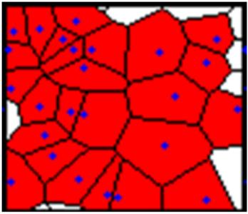
Figure 1. Voronoi diagram representing randomly distributed schools with surrounding catchment areas. Each Voronoi cell represents a school neighborhood whose size is determined by the number of geographical locations encompassed by the cell. A school is located at the center of each cell. - 2.4
- We want to know whether ethnic preferences have a similar effect on school segregation as they have on residential segregation and how this is affected by a simultaneous preference for a short distance between home and school. To model the ethnic preference component of agents' preference function we build on previous work by Zhang (2004) and use a single-peaked linear function that maps the local proportion of members of the same group on the attractiveness of the school or residential location for an agent. An example is depicted in figure 2.
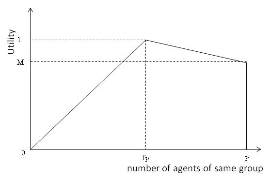
Figure 2. Ethnic preference for composition of neighborhood or school. M is a constant factor representing the desirability of 100% own ethnic group, and f represents the fraction of in-group members of the neighborhood or school population that is optimal for the agent. - 2.5
- The illustrated function peaks at n=f p where f is the optimal fraction of the total number of agents (p) in the local composition. Notice that the agents can actually prefer a certain level of local ethnic integration above perfect segregation, reflecting the aggregate-level empirical pattern in studies on residential preferences in the U.S. (Clark and Fossett 2008). More technically, on the left side of n=f p, the function is linearly increasing, whereas on the right side of this point, it is linearly decreasing. Agents always obtain a utility of zero if the local composition comprises only out-group members, and they obtain a utility of M > 0 when the local composition comprises only in-group members.
- 2.6
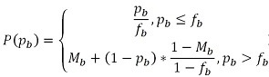
- Formally, we model ethnic preference P with the function given in equation (1).
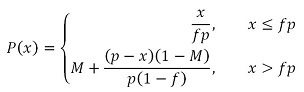
(1) where p is the total number of agents in the neighborhood or school, and x the local number of agents of the own group.
- 2.7
- In the school model, agents can evaluate a school not only in terms of its ethnic composition, but also in terms of the distance between their residential location and the school. More explictly, an agent's utility U for the school chosen is obtained from a Cobb-Douglas utility function. Technically,
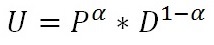
(2) where α is a parameter which controls how much weight is put on the ethnicity preference (P) relative to the distance preference (D). P is obtained from equation (1), D represents the "nearness" of the school, implemented as the mirror image of the geographical distance between residential location of the household and the school. Technically, the nearness of school i to agent j, Di,j, is given by
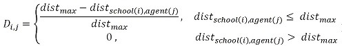
(3) where distmax is a maximum distance that serves as normalization factor and dist school(i),agent(j) is the distance between the agent's residential location and the school. Throughout this paper, we assume distmax to be the maximum distance between two locations in the geographical space. For a two dimensional grid with N × N locations embedded on a torus distmax = N/√2.
- 2.8
- In the actual decision function, the utility an agent would obtain from choosing a certain residential location (or school), is compared against a satisfaction threshold represented by a further model parameter (T). Only when P < T is the agent assumed to be sufficiently dissatisfied with the residential location or school to consider whether to move to a different location (or change school). With this, we follow Schelling's original approach in assuming that agents are "satisficing" (Simon 1956).
- 2.9
- We first implemented a simple Schelling type model (Model 0) of residential segregation, then followed by two school segregation models without (Model 1) and with distance preferences (Model 2). In all models, ethnic groups can differ in their ethnic preferences, but are assumed to be homogenous internally. Distance preferences are meaningless in model 0 and are not taken into account in model 1, i.e. α = 1 in both models. Throughout, all agents are initially assigned a random location in the world.
- 2.10
- Residential model and school model are alike in most features of model initialization and model dynamic. The following applies to both models unless explicitly noted otherwise. The maximum number of agents populating the model is Nmax = 10.000. Population size is throughout assumed to be N = 8700, a value that falls within a broader range of filling rates for which we found sufficient movement of agents to obtain model convergence in reasonable time. The distribution across the ethnic types A and B is varied in the simulation experiments. In every round of the simulation, 500 randomly chosen agents can change their location (or school). However, the number of agents that actually change their location is limited by the number of free spaces. More precisely, for each selected agent, we calculate satisfaction with the current local unit chosen based on the utility function given by equations (1) and (2), the current local ethnic composition and their ethnic preferences. In the residential model, we define an agent's neighborhood as being a diamond-shaped neighborhood of the residential location. The neighborhood encompasses the set of locations whose center points fall within a certain Euclidian distance around the center point of the focal cell. In figure 3 we illustrate the neighborhood for a radius r = 3. The local proportion of in-group and out-group members is calculated relative only to the numbers of cells (or "slots" of a school) that are actually occupied.
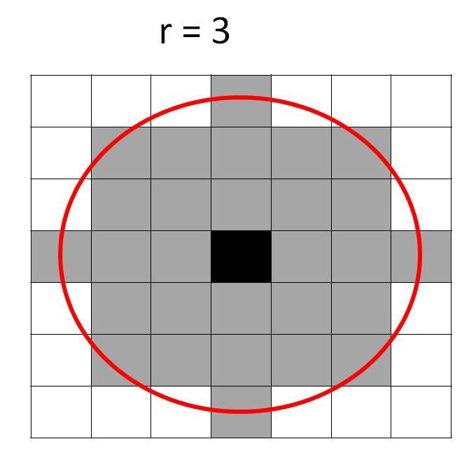
Figure 3. The squares with grey color show the cells that fall within the residential neighborhood of the black center cell for a radius of r = 3. - 2.11
- If the satisfaction with the local composition falls below the satisfaction threshold T then the agent will move to a random location where his requirements are satisfied, if one is available. In the residential model, this new location is selected out of a maximum of 100 randomly chosen empty locations. In the school model, all schools that still have empty slots are considered in random sequence. The agent will move to the first found location out of the locations investigated for which his utility exceeds the threshold T. If, however, a satisfactory location is not found in the locations that were searched, the search will continue. We included the assumption that the search can continue in order to model the notion that in adaptive decision making actors adapt not only their behavior but also their aspirations over time to the experiences they make (e.g. Macy & Flache 2002; Bendor et al. 2003). More concretely, when dissatisfied agents find no alternative satisfactory location they will, in the residential model, randomly select another 100 empty locations to be inspected. In the school model, all schools which still have empty slots are re-considered. In this second pass, the agent will move in both models if the utility that would be obtained at the inspected location exceeds the utility derived at the current location, even if the utility at the destination would fall below the satisfaction threshold T. In other words the agent will move to the first location he finds where he is happier. If a better location is not found then the agent will stay. Within one round the agents investigating a new location calculate their utility function based on the population distribution that is present at the beginning of the round. This models the assumption that agents who attain moving options within the same round take their decisions quasi simultaneously. An agent is, however, unable to move to a location or occupy a slot at a school that has been claimed by another agent in the same round. All agents will move simultaneously to their selected locations or new schools at the end of the round.
- 2.12
- For the school model in particular, we assume each agent has one child that initially is enrolled at the closest school, the school located at the generator point of the Voronoi cell in which the residential location of the household falls. This means that initially the composition and filling-rate of a school is representative of its neighborhood.
Segregation indices
- 2.13
- To quantify segregation in both models, we devised a set of measures based on the dissimilarity index (Massey and Denton 1988). This index expresses how much, taken across a set of local units, the ethnic composition of the local unit differs from the population composition on average. Maximal segregation occurs when the index obtains a value of one, the theoretical lower bound is zero. Equation (4) shows how the basic measure of the dissimilarity index is calculated.
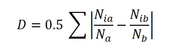
(4) In equation (4), Nix expresses the number of members of ethnicity "x" (A or B) of the local unit "i" (neighborhood or school) and Nx is the number of members of that group in the overall population. For the school model, we use schools as local unit for calculating the index that we refer to as the "school segregation index". For comparison with the school model, we distinguish two segregation measures for the residential model which are differently "fine grained". The "variable neighborhood index" uses the neighborhood defined by the radius r that agents use to evaluate neighborhood composition. Finally, the "school-neighborhood index" takes school-neighborhoods as local unit, for comparison with the school segregation index.
Results
- 3.1
- Schelling's model shows that theoretically, segregation may arise even in conditions where a non-segregated distribution would satisfy all individuals. We wanted to know whether and under which conditions this also applies for the school model. To begin with, we compare the residential model to the school model without distance preferences. The school model without distance preference is similar to a "bounded neighborhood" version of the residential model and should thus produce similar results. To assess this, we first describe a baseline experiment in which we compare the school model without distance preferences with the residential model and identify the conditions under which the behaviors of both models align. Then, we explore whether the effects that we found without distance preferences hold up when we introduce preferences for nearby schools into the school model, under various different conditions.
Baseline experiment
- 3.2
- To establish a baseline for comparison, we began by simulating a prototypical residential segregation dynamic. We chose an ethnic population composition and preference parameters such that individuals of both groups would be satisfied if the local ethnic composition at their residential location equals the overall ethnic composition of the population. For this, we assumed that members of both groups reach their maximal utility of U=1 with 70% in-group members (i.e. fa = fb = 0.7). Furthermore, they reach a utility of U=M=0.8 with 100% in-group members. To assure that these segregationist preferences are "mild", we set the satisfaction threshold to T=0.4. As figure 4 below illustrates, both groups can still be satisfied with a local out-group majority under this parameterization.
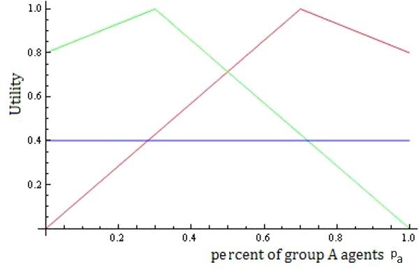
Figure 4. Green line represents the preference function for group B with peak at pb = 1-fb. (Mb = 0.8, fb = 0.7). The red line represents the preference function for group A with peak at pa = fa. (Ma = 0.8, fa = 0.7). The blue line illustrates the satisfaction threshold T = 0.4. - 3.3
- Figure 4 shows that for group A, utility falls below the satisfaction threshold T only when the local proportion of group A members is less than pa,min = fa * T = 0.28, while group B members will only be dissatisfied when the proportion of group A members exceeds pa,max = 1 − T fb = 0.72 (for a formal derivation see further below and proof in the appendix, local equilibrium condition A). To obtain for the baseline simulation an initial condition where both groups can be satisfied when the local ethnic mix is representative of the overall population distribution, we assumed that groups A and B have equal size. Finally, following most previous work on Schelling-type residential segregation dynamics, agents focus in the residential model on a local environment that represents only a small part of the overall world. We set the radius for the residential neighborhood to r = 1.5, creating local neighborhoods that encompass only 8 neighbors or 0.08% of all cells of the world.
- 3.4
- Starting from a randomly mixed initial population we found that segregation establishes after ~ 300 rounds and then stabilizes. This pattern is prototypical for Schelling-type models of residential segregation. Figure 5 shows the final distribution of agent-types across space in a prototypical run. After 300 rounds, the average proportion of neighbors of the own type had increased to 67% from an initial 50%. While the average neighborhood composition falls within the acceptable range for both groups, this average does not reflect the actual segregation. After 300 iterations, the proportion of agents for whom the local composition falls outside of the range that is acceptable for both groups has increased to approximately 38% from an initial 29%. Moreover, 86% of the free locations have a local composition that falls outside this range, showing that further moves are likely to increase segregation.
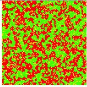
Figure 5. State of the neighborhoods after 300 iterations. Initial 50%-50% population mix, 8700 agents, f = 0.7, M = 0.8 T = 0.4. - 3.5
- Segregation increases in this condition beyond the initial random mix because initially not every local residential neighborhood is a perfectly representative sample of the population mix. Local residential neighborhoods contain only up to 8 out of the 8700 agents of the population. Thus, there are initially a number of agents for whom the proportion of group A members in their local residential neighborhood does not fall within the acceptable range. We approximated the probability that at a randomly chosen location the initial proportion of group A members falls outside of the acceptable interval [0.28, 0.72] with the cumulative density function of the binomial distribution. This yields a probability of approximately 0.29. This suggests that the number of agents that are not satisfied with their initial residential neighborhood is large enough to set off a cascade of consecutive migrations in which local neighborhoods then develop gradually higher concentrations of either A or B agents.
- 3.6
- Next we investigated whether a similar segregation dynamic would arise from the school segregation model without distance preferences (α= 1) under otherwise identical conditions. At the outset, every household from a school-neighborhood assigned its one child to the neighborhood's school so that schools mirrored the randomly mixed initial ethnic composition of neighborhoods. We found that there was virtually no change in the ethnic composition over time. Schools remain ethnically integrated throughout.
- 3.7
- The residential dynamic differs from the school-choice dynamic in this initial example because schools constitute much larger 'local neighborhoods' than the residential neighborhoods with radius r = 1.5 of the residential model. The size of schools varies between about 100 and 800 "slots". For this size, obtaining local concentrations of group A members outside the range that satisfies both groups is virtually impossible from a random start. Approximation of the probability yields an approximate probability below 10-5 for this event.
- 3.8
- Model dynamics differ between residential and school model, because schools recruit their initial population from a neighborhood much larger than the local residential neighborhoods. School neighborhoods are more representative of the overall population mix and match thus – in the baseline condition – the ethnic preferences of all parents in the population. Laurie and Jaggi (2003) reported a similar result in their analysis of the effects of the size of agents' local neighborhoods in their residential Schelling model. But their work also pointed to an interesting interplay between the effects of neighborhood size and the restrictiveness of ethnic preferences. The authors found that a larger neighborhood size increases segregation when agents' satisfaction threshold was relatively low, but a larger neighborhood size could increase segregation when agents had more demanding ethnic preferences. The larger the neighborhood size, the more the local composition is a representative sample of the overall population. Larger neighborhoods thus temper segregation when the overall population distribution would satisfy agents also locally, but they foster segregation otherwise.
- 3.9
- To assess whether the interplay between ethnic preferences, population composition and neighborhood size can explain the differences that we found between the residential model and the school model without distance preferences, we conducted a simulation experiment in which we varied both the overall population composition and neighborhood size, leaving ethnic preferences unchanged relative to the previous experiment (f = 0.7, M = 0.8, T = 0.4). Before presenting results of the experiment we will, in the following, first present a more general analysis of the conditions under which an integrated local ethnic composition for both groups can be expected to be stable when agents are indifferent with regard to the distance from a school. This analysis serves to explain the selection of conditions that we compared in the subsequent simulation experiment.
Conditions for stable ethnic integration without distance preferences
- 3.10
- In the subsequent experiment, we varied both the ethnic composition of the population and the neighborhood size in the residential model. The key idea is that the residential dynamic should become more similar to the school choice dynamic when the size of residential neighborhoods becomes larger. To assess this, we distinguish three different population compositions representing conditions where, respectively, a) the representative local mix satisfies well agents of both groups, b) representative local compositions can still satisfy both groups but small local deviations from the overall ethnic composition suffice to render at least one group dissatisfied, and c) a representative local composition dissatisfies at least one group.
- 3.11
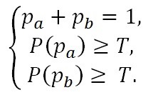
- To operationalize the three different compositions, we first analyzed under which conditions members from both groups obtain at a certain location a utility that exceeds their satisfaction threshold T. If this happens, no agent will leave the location. For simplicity, we assumed that both groups hold the same satisfaction threshold and we impose the plausible restriction that being in the local minority is suboptimal for both groups (1-fb ≤ 0.5 and fa ≥ 0.5). Furthermore, we neglected the actual size p of the local unit and considered only the local proportions pa and pb of members of group A and B, respectively. Finally, empty slots are neglected such that pa = 1- pb.
- 3.12
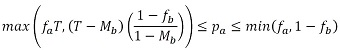
- Intuitively, figure 4 indicates that simultaneous satisfaction of both groups is only possible when the satisfaction threshold (T) falls below the utility level that agents obtain at the proportion pa,x where both groups are equally happy with the local mix. For any other local composition either group A or group B obtains a lower utility level. More technically, pa,x is the proportion of members of group A at which the left branch of the utility function of group A intersects with the right branch of the utility function of group B, where the latter utility function is expressed as a function of the out-group proportion pa = 1- pb. Mathematically, the satisfaction threshold T can only be below the utility obtained at this intersection point when[2] T ≤ 1/(fa+fb).
- 3.13
- Our analysis of the conditions for local integration confirms that the preference parameters that we used in the baseline experiment allow for integrated compositions. With fa = fb = 0.7, we find that T = 0.4 ≤ 1/(fa+fb) ≅ 0.714. Further analysis yields the lower and upper boundaries pa,min and pa,max, respectively, of the interval within which utility exceeds T for both groups. These boundaries are obtained from equation (1) as pa,min = fa T and pa,max = 1 – T fb. For the regime in which both groups should be satisfied with representative compositions, we thus need to choose a population composition between pa,min = fa T = 0.7 * 0.4 = 28% group A and pa,max = 1 – T fb = 1-0.28 = 72% group A. This leads us to adopt the following three population distribution regimes for the experiment. An "integration regime" is imposed with the even ethnic distribution 50-50, a "precarious integration regime" is generated with a distribution in which group A is the majority group in a 70-30 mix and, finally, we impose a "segregation regime" with an ethnic distribution 90-10 in favor of group A. Notice that only with the "segregation regime" at least one group (B) would always be dissatisfied with a local distribution representative of the overall population.
- 3.14
- To be sure, the conditions identified above are neither sufficient nor necessary for obtaining an equilibrium for the dynamics of either model. The condition T ≤ 1/(fa + fb) is not sufficient to guarantee system stability because local compositions may differ from the global population mix, as we have seen in the baseline simulation of the residential model. The condition is also not necessary for a stable outcome, because fully segregated outcomes can also be stable equilibria of the system as long as T ≤ M for both groups. Nevertheless, we can expect that an integrated initial distribution is more robust to the extent that the overall composition falls more into the interior of the interval [pa,min, pa,max] and that local neighborhoods in the residential model are larger. This is what we will explore next.
Joint effects of population composition and residential neighborhood size
- 3.15
- In the next experiment, we varied the radius of the local residential neighborhoods in three steps, from r = 1.5 over r = 5 to r = 11. These steps generate neighborhoods that, respectively, comprise 8, 80 and 376 locations (0.08%, 0.8% and 3.76% of all locations, respectively). For r = 11 neighborhood size is approximately equal to school sizes, which range between about 100 and 800. For each radius condition, we varied the ethnic composition of the overall population, changing across the integration regime (50-50), the precarious integration regime (70-30) and the segregation regime (90-10). All other parameters remained equal to those we used in the baseline experiment (N = 8700, fa = fb = 0.7, Ma = Mb = 0.8, Ta = Tb = 0.4 and α = 1).
- 3.16
- Figure 6 presents results of the experiment for the residential model. The figure shows for all 9 conditions the change of three segregation indices: the school-neighborhood index, the variable neighborhood index, and the dissimiliarity index based on local neighbourhoods with radius r = 1.5. For reliability, segregation indices are averaged across 100 independent replications per condition. We find the variance of the indices across the independent replications to be in the order of 0.005, which is indistinguishable on the displayed plots, this being the reason to display only the means.
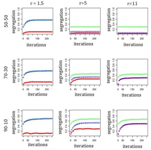
Figure 6. Segregation indices for residential model for three different radius values: r = 1.5, 5, 11 and for three different ethnic compositions: 50-50, 70-30, 90-10. The blue line is the variable neighborhood index, the green line is the dissimilarity index based on local neighborhoods with radius r=1.5 and the red line is the school segregation index. ( N = 8700, fa = fb = 0.7, Ma = Mb = 0.8 and Ta = Tb = 0.4). - 3.17
- The first row of figure 6 confirms the expectation that larger neighborhood size suppresses segregation in the 50-50 population composition that we used in the baseline experiment. Increasing the radius from r = 1.5 to r = 5 considerably reduces segregation and at r = 11 the initial randomly mixed condition was stable, like in the school model.
- 3.18
- Results also support that initial integration can be better sustained with larger neighborhoods and an overall population mix that falls more into the interior of the interval [0.28, 0.72]. Except for the smallest neighborhood radius of r = 1.5, segregation increases less in the integration regime (50-50) than in the precarious integration regime (70-30) and most in the segregation regime (90-10). Moreover, for all three regimes the increase of segregation is strongest for the smallest neighborhood radius (r = 1.5). Finally, in the segregation regime representative local neighborhoods cannot be stable and, accordingly, larger neighborhood size has no effect on the stability of the initial integrated state across all three neighborhood sizes. The increase of the school-neighborhood index in particular shows that the segregation occurs increasingly at a macroscopic scale as neighborhoods get bigger.
Effects of population composition and distance preferences in the school model
- 3.19
- School choices reflect not only parents' preferences for ethnic compositions but also preferences for nearby schools. Our analysis for the residential models has shown that even when neighborhoods are as large as they are in the school model, there is a potential for emergent segregation in the precarious integration regime and the segregation regime. But when parents prefer nearby schools this may curb tendencies towards self-organized school segregation if the initial distribution of households across geographical space is ethnically integrated. Households who are dissatisfied with the ethnic composition of their local school may not find a more attractive school if all schools with a more favorable ethnic composition turn out to be too far away. We wanted to know whether a preference for nearby schools can curb cascades towards segregation in those regimes.
- 3.20
- In a first experiment, we simulated with the school model the precarious integration condition (population mix 70-30) for which we know that a perfectly integrated outcome can be satisfactory for all agents, but is hard to sustain from a random start. Across different conditions, we gradually changed in steps of 0.2 the weight α that parents put on optimizing ethnic composition relative to minimizing distance. The parameter was varied between α = 0 and α = 1. Figure 7 shows results based on averages of 100 independent replications per condition.
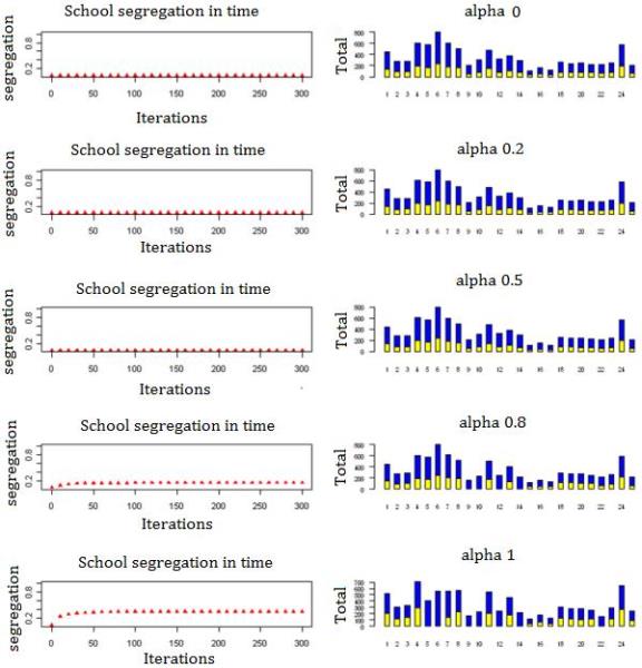
Figure 7. Left side: Change of school segregation index; Right side (bar charts): Ethnic composition and size of the 25 schools after 300 iterations for illustrative single-run. N = 8700, with a 70-30 ethnic composition (fa = fb = 0.7, Ma = Mb = 0.8, T = 0.4). - 3.21
- Figure 7 shows how a preference for nearby schools can suppress the trend towards increasing school segregation that we observed when parents were indifferent towards distance, all other things being equal. The results for α between and including α = 0 and α = 0.5 show that the initial integrated state is preserved. Only when distance minimization is less important to the simulated parents than the ethnic composition, we observe that segregation increases noticeably above its initial level of zero. However, even for α = 0.8, the dissimilarity index for the final state is only about half as large as for the case when parents were assumed to be indifferent to distance (α = 1.0). This effect is also reflected by the number of schools that is ethnically homogenous in the illustrative runs shown in the right column. For the conditions with α ≤ 0.5, both groups are represented at all schools. However, with α = 0.8, four schools end up as "majority only", and with α = 1.0 this number has increased to seven schools. Thus, without a preference for nearby schools, also the school model can generate unintended segregation in the same way as the residential model.
- 3.22
- In the next experiment, we compared the effects of distance preferences across the three regimes of population composition, using the same set of preference parameters for ethnic compositions than before.
- 3.23
- Figure 8 shows the results for the change of the school segregation index, for the three regimes of the initial population composition. Per regime, we simulated three values for the weight of the preference for nearby schools, α = 1 (only ethnic composition matters), α = 0.5 (equal weight for ethnic composition and distance), and α = 0.2 (mainly distance matters). Results are based on 100 independent replications per condition.
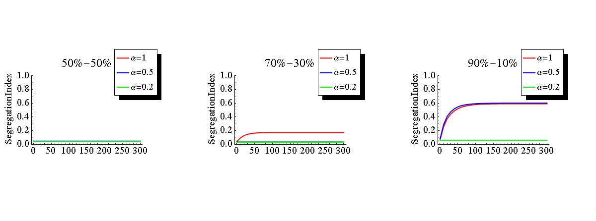
Figure 8. Change of school segregation index for three different regimes of ethnic compositions and α = 1 (red), α = 0.5 (blue), α = 0.2 (green): 50-50, 70-30, 90-10. N = 8700, fa = fb = 0.7, Ma = Mb = 0.8 and Ta = Tb = 0.4. - 3.24
- When only ethnic composition matters to parents (α =1), the initially integrated state persists only in the integration regime (50-50), like for the residential model with large neighborhood radius. At this level of α, the increase of segregation observed in the other two regimes is stronger for the segregation regime (90-10) than for the precarious integration regime (70-30). This pattern changes, however, when we put a higher weight on agents' preference for nearby schools. When distance and ethnic composition have an equal weight (α = 0.5), segregation increases above its initial level only in the "segregation-regime", while – as found in the previous experiment - in the "precarious integration regime", agents' preference for nearby schools prevents segregation. Finally, in the condition where agents put more weight on the distance to school than on ethnic composition (α = 0.2), segregation arises in none of the regimes.
Joint effects of agents' "tolerance" for out-group members and distance preferences
- 3.25
- Throughout the experiments presented before, we used the same set of parameters for agents' ethnic preferences and only varied the weight of their preference for nearby schools. A key idea in research based on Schelling's segregation model is that segregation can arise even when agents are quite tolerant of the presence of out-group members in their local environment. We wanted to know to what extent our models can generate this result, and whether a preference for nearby schools dampens effects of increasing intolerance on segregation. For this purpose, we performed for both the residential and the school segregation model a series of simulations varying the optimal fraction of in-group members f for both ethnic groups over the range of possible values, from very tolerant (small f values) to intolerant (large f values). More precisely, the values of f were varied for both groups across all recombinations of (fa,fb) that resulted from the values of f = 0.1, 0.3, 0.5, 0.7, 0.9. For the school model, we compared the effects of variation in f between a condition in which only ethnic composition mattered to agents (α = 1) and one in which both ethnic composition and travelling distance to school had equal importance (α = 0.5).
- 3.26
- The simulations were performed using a 70-30 population composition, with otherwise the same parameter values as used in the previous experiments (N = 8700 agents, Ma = Mb = 0.8, T = 0.4). For the residential model, the radius was set to r = 1.5. The results of the simulations are presented in figure 9, where, subfigures (a) and (b) show results for the residential model with the school-neighborhood index, and the variable neighborhood index, respectively. Subfigures (c) and (d) chart results for the school model with the school segregation index, without (α = 1) and with (α = 0.5) preferences for nearby schools, respectively. For reliability, segregation indices are averaged across 100 independent replications per condition, where each replication was run until segregation stabilized.
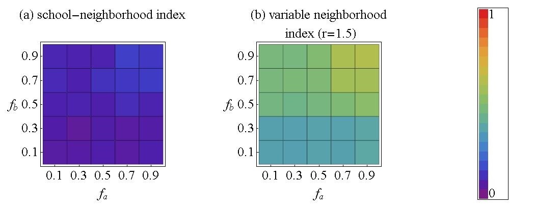
Figure 9. School-neighborhood index (a) variable neighborhood index (b) school segregation index without preference for distance (α = 1) (c) and school segregation index with preference for distance (α = 0.5) (d) for different (fa - fb) combinations. All other parameters are equal to the previous experiments. N = 8700, Ma = M = 0.8 and Ta = Tb = 0.4. For the residential model, r = 1.5. - 3.27
- Intuitively, we expect that segregation increases when agents' tolerance for out-group members decreases. This expectation is broadly consistent with the results presented in figure 9, but there are interesting deviations from the expected pattern. For school segregation, we observe in graph (c) that even without a preference for nearby schools values of the school segregation index remain very low (smaller than 0.05) unless minority members find an in-group fraction of fb = 0.7 or more optimal. This reflects how ethnic preferences affect the probability that in the initial random mix a school is unacceptable for either the majority or the minority group. From equation 1 we can derive that with the threshold of T = 0.4, a representative school (70% A) is acceptable for the majority group A at any value that the parameter fa can take. However, this is different for the minority group B. From the experiments reported in figure 8 we know that at fa = fb = 0.7 a perfectly representative school composition would just satisfy the minority, but segregation nevertheless unfolds because in some schools the initial minority is slightly smaller, due to random chance. With fb = 0.5 or smaller this does not yet happen, because minority members are well satisfied with the initial mix, but for fb = 0.7 or more local dissatisfaction triggers a cascade of movements of minority members out of integrated schools which eventually results in the high levels of school segregation that we find for those conditions. In this region of the parameter space, the value of the school segregation varies between 0.217 (at fa = fb = 0.7) and 0.341 (at fa = 0.7, fb = 0.9). A comparison of this pattern with the results we obtain for residential segregation at local scale (graph (b), variable neighborhood index) shows that the results are qualitatively similar in that mainly higher fb increases local residential segregation. At the same time we find that local residential segregation responds more smoothly to changes in agents' preference function than school segregation without preferences for nearby schools does. The reason is that the initial composition of small local neighborhoods varies more around the overall population mix, such that changes in agents' tolerance noticeably affect the probability that in some local regions at least one of the two groups is dissatisfied with the local mix and starts to move out. Residential segregation at the macroscopic scale of school-neighborhoods (graph (a), school-neighborhood index), finally, is largely unresponsive to levels of ethnic tolerance because with an r=1.5 for the utility function, segregation in small homogenous regions is enough to satisfy agents, therefore reducing the probability of forming larger homogenous regions. Only when both groups have very demanding preferences (f > 0.7), a slight tendency towards the formation of larger segregated regions is noticeable (school-neighborhood index > 0.1).
- 3.28
- Subfigure (d) shows how a preference for nearby schools suppresses effects of agents' tolerance for out-groups and prevents segregation. With a weight of 1-α = 0.5 of the distance between home and school, the effects of f all but disappear. For all combinations of fa and fb segregation levels remain very low, close to the initial level of segregation obtained for a random distribution of agents. This is particularly remarkable for the condition of fa = fb = 0.9, in which a statistically representative school is no longer acceptable for members of the minority. (Figure 9 school segregation index α =0.5.)
Conclusions
- 4.1
- We have developed in this paper a stylized model for school choice dynamics that builds on the same principles as the well known Schelling model of residential segregation. Our analysis of the differences between the Schelling type residential segregation model and the school model showed that integrated distributions that are in line with agents' preferences are much more robust in the school model when the size of residential neighborhoods is small relative to the size of the catchment areas of schools. At the same time, when the overall ethnic composition of the population is relatively unfavorable compared to individual ethnic preferences, preference dynamics that generate high levels of unintended segregation unfold in both models under comparable conditions. For the school choice model, these results reflect Schelling's (1978) analysis of the tipping process of bounded neighborhoods. Bounded neighborhoods can be seen as similar to schools in our school model. In this sense, the results we obtained in the first part of the paper mainly serve to demonstrate that our school model aligns with results that have previously been obtained for residential segregation, as long as we neglect parents' preferences for nearby schools.
- 4.2
- An important difference between residential segregation dynamics and school segregation dynamics is that parents choose a school within some distance from their home, while not changing their residential location. The distance of schools from home can thus matter for parents' choices and be a factor that tempers segregation dynamics. This was illustrated by the results that we obtained when we introduced a preference for nearby schools in addition to the ethnic preferences of the Schelling model. We found that this curbed segregation in an initially integrated population that would have segregated when parents' choices had only been driven by ethnic preferences. Similarly, when we varied the population composition and agents' tolerance for outgroup members, we found that integrated distributions were preserved under a much broader range of conditions than in the absence of a preference for nearby schools. An interesting question for future research that follows from this is whether and to what extent the high levels of school segregation observed in many Western countries are mainly due to residential segregation rather than to 'Schelling-type' preference dynamics.
- 4.3
- We deliberately used highly stylized models to obtain a clear comparison with the well-known Schelling dynamic. Due to this, there are number of limitations of our work that point to directions for future research. To begin with, we neglected heterogeneity in agents' preferences within ethnic groups, unlike in Schelling's (1978) analysis of bounded neighborhoods where the distribution of agents' tolerance threshold is the main parameter of interest. Our homogeneity assumption may lead to an overassessement of the stability of ethnic integration, because, as Schelling's analysis suggests, even if a local ethnic mix satisfies the average individual of a group, there can still be individual members with more demanding preferences who leave the neighborhood or school and thus trigger a cascade towards segregation. Moreover, the deterministic choice function of our model does not account for the possibility of random heterogeneity in agents' preferences. To address this, future work should integrate random utility assumptions similar to those used by Zhang (2004a) into our school segregation model.
- 4.4
- The modelling work presented here is just the first step in a broader project. In future research, we aim to further elaborate our school segregation model with the goal to make it applicable for modelling the dynamics of ethnic school compositions that actually can be observed empirically for primary schools in the Netherlands. This requires to further extend the model to incorporate a broader spectrum of preference arguments that parents are known to take into account from empirical research, such as preferences for schools with perceived high educational achievements or specific religious denominations. It also requires to link available empirical information on the corresponding school characteristics as well as on residential ethnic compositions, and geographical locations of schools and school neighborhoods to the model. We believe that integrating empirical information with theoretical models of segregation is a promising direction to assess competing explanations of school segregation (e.g. a preference based vs. a residential segregation based account) and to explore theoretically what the effects of policies could be that have been proposed to counter school segregation.
Appendix
- A.1
- We deduce analytically the conditions under which given f and M for both groups a local composition is satisfactory for both groups. We assume throughout that agents are indifferent with regard to distance, i.e. α =1.
- A.2
- We write equation (1) separately for each group. For group A this yields:
(5) - A.3
- For group B we obtain:
(6) - A.4
- Also we impose that pa + pb = 1 and assume that both groups are satisfied. In the following we analyze, under which conditions mutual satisfaction can hold. We also call mutual satisfaction the condition for "local equilibrium".
(7) - A.5
- We re-write equation (6) as follows:
(8) - A.6
- We distinguish further four different global outcome possibilities for equation (3) and equation (6).
- For
pa ≤ fa and (1-pa) ≤ fb, we obtain:
(9) Using the condition that both groups are satisfied for the given proportions of ethnic groups, we obtain
(10) The conditions implied by equations (9) and (10) can be summarized as follows for the parameters fa and fb:
(11) Out of this we obtain as follows a condition for satisfaction of both groups:
leading to the following condition for the local proportions pa of members of group A

(12) - For pa ≤ fa and (1-pa) > fb, we obtain:
(13) Out of equation (13) together with the initial conditions for the proportion of population of group A and group B, we write, in a similar manner as for case A, the local equilibrium condition as follows:
- pa > fa and (1-pa) > fb, for these we have the following:
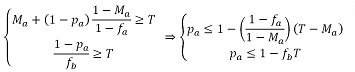
(14) Out of this we write the equilibrium condition as follows:
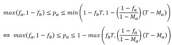
(15) - pa > fa and (1-pa) > fb, implying that 1>(fa + fb)for these we have the following:
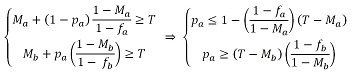
(16) Out of this we can write the equilibrium condition as follows:
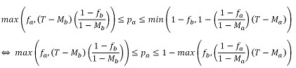
(17)
- For
pa ≤ fa and (1-pa) ≤ fb, we obtain:
- A.7
- We can thus state that the system is in equilibrium if it obeys any of the conditions given in Eq. 12, Eq.14, Eq.16, or Eq.18 for all the schools or neighborhoods at the same time.
- A.8
- We can assume that fa = fb; Ma = Mb. The equilibrium conditions can also be used to extract further conditions for the parameters f, with respect to the threshold T.
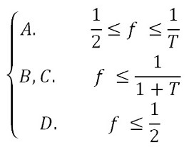
(18) The parameter f represents the percent of own color population. We can safely assume that f ≥ 1/2 (nobody likes to be in a minority), so condition D is usually invalid.
Notes
-
1 The C++ code of the model can found at http://www.openabm.org/model/3842/version/1/view.
2 Formal proofs for the theorems presented in this section can be found in the appendix.
References
-
AXTELL, R., Axelrod R., J.M. Epstein and M.D. Cohen (1996). "Aligning Simulation Models: A Case Study and Results.", Computational and Mathematical Organization Theory 1(2), 123–141. [doi:10.1007/BF01299065]
BAKER, J., Denessen, E., Peeters, D., and Walraven, G. (2011). "International Perspectives on countering school segregation." Antwerpen-Apeldoorn, Uitgeverij Garant, ISBN 978 90 4412 6945.
BENDOR, J., Diermeier, A., and M. Ting. 2003. "A Behavioral Model of Voter Turnout." American Political Science Review 97: 261–280. [doi:10.1017/S0003055403000662]
BELL, C. (2009). "Geography in Parental Choice." American Journal of Education 115, 493–521. [doi:10.1086/599779]
BOVENS, M. and Trappenburg, M. (2006). "Segregation through Anti-Discrimination: How the Netherlands Got Divided Again." Chapter 4 in: Verweij, M. and Thompson, M. (eds.). Clumsy Solutions for a Complex World. Governance, Politics and Plural Perceptions. Basingstoke (CY): Palgrave Macmillan.
CBS [Statistics Netherlands] (2007). Jaarboek onderwijs in cijfers 2008 [In Dutch, Annual statistical school report 2008]. Voorburg/Heerlen: Centraal Bureau voor de Statistiek.
CLARK, W. A. V. and Fossett, M. (2008). "Understanding the social context of the Schelling segregation model." Proceedings of the National Academy of Sciences of the United States of America 105(11), 4109–4114. [doi:10.1073/pnas.0708155105]
COENDERS, M., Lubbers, M., and Scheepers, P. (2004). "Weerstand tegen scholen met allochtone kinderen. De etnische tolerantie van hoger opgeleiden op de proef gesteld" [Resistance against schools with non-western minority pupils]. Mens en Maatschappij 79, 124–147.
DENESSEN, E., Driessen, G. and Sleegers, P. (2005) "Segregation by choice? A study of group-specific reasons for school choice." Journal of Education Policy, 20(3), 347–368. [doi:10.1080/02680930500108981]
FLACHE, A., and Hegselmann, R. (2001). "Do Irregular Grids make a Difference? Relaxing the Spatial Regularity Assumption in Cellular Models of Social Dynamics." Journal of Artificial Societies and Social Simulation 4. https://www.jasss.org/4/4/6.html
FOSSETT, M. (2006a). "Ethnic preferences, social distance dynamics, and residential segregation: Theoretical explorations using simulation analysis." Journal of Mathematical Sociology 30, 185–274. [doi:10.1080/00222500500544052]
FOSSETT, M. (2006b) "Including Preference and Social Distance Dynamics in Multi-Factor Theories of Segregation" Journal of Mathematical Sociology 30, 3–4, 289–298. [doi:10.1080/00222500500544151]
FOSSETT, M., and Warren, W. (2005) "Overlooked Implications of Ethnic Preferences for Residential Segregation in Agent-based models" Urban Studies 42–1893. [doi:10.1080/00420980500280354]
GRAUWIN, S., Bertin, E., Lemoy, R., and Jensen, P. (2009). "Competition between collective and individual dynamics." Proceedings of the National Academy of Sciences of the United States of America 106, 20622–20626. [doi:10.1073/pnas.0906263106]
HATNA, E. and Benenson, I. (2012). "The Schelling Model of Ethnic Residential Dynamics: Beyond the Integrated - Segregated Dichotomy of Patterns." Journal of Artificial Societies and Social Simulation 15 (1) 6 https://www.jasss.org/15/1/6.html.
HEGSELMANN, R. and Flache, A. (1998). "Understanding complex social dynamics: a plea for cellular automata based modeling". Journal of Artificial Societies and Social Simulation 1. http://www.soc.surrey.ac.uk/JASSS/1/3/1.html.
HEGSELMANN, R, A. Flache, V. Mö ller, (2000). "Cellular Automata Models as Modelling Tool". pp. 151–178 in: Suleiman R., K.G. Troitzsch, N. Gilbert (eds.). Tools and Techniques in for Social Science Simulation. Heidelberg: Physica.
KARSTEN, S., Ledoux,G., Roeleveld, J., Felix, C. and Elshof, D. (2003). "School choice and ethnic segregation." Educational Policy 17, 452–477. [doi:10.1177/0895904803254963]
KARSTEN, S., Felix, C. , Ledoux, G., Meijnen, W., Roeleveld, J. and Van Schooten, E. (2006). "Choosing segregation or integration? The extent and effects of ethnic segregation in Dutch cities." Education and Urban Society 38, 228–247. [doi:10.1177/0013124505282606]
KRISTEN, C. (2008). "Primary School Choice and Ethnic School Segregation in German Elementary Schools." European Sociological Review 24, 495–510. [doi:10.1093/esr/jcn015]
LAURIE, A.J. and Jaggi, N.K. (2003). "The role of 'vision' in neighborhood racial segregation: A variant of the Schelling segregation model." Urban Studies 40, 2687–2704. [doi:10.1080/0042098032000146849]
LOGAN, J., Oakley, D. and Stowell, J. (2008). "School Segregation in Metropolitan Regions, 1970–2000: The Impacts of Policy Choices on Public Education." American Journal of Sociology 113, 1611–1644. [doi:10.1086/587150]
MACY, M. W. and Flache, A. (2002). "Learning Dynamics in Social Dilemmas". Proceedings of the National Academy of Sciences U.S.A. 99(10), 7229–36. [doi:10.1073/pnas.092080099]
MACY, M. W. and Willer, R. (2002). "From Factors to Actors: Computational Sociology and Agent-Based Modeling" Annual Review of Sociology , 28, 143–166. [doi:10.1146/annurev.soc.28.110601.141117]
MACY, M. W. and van de Rijt, A. (2006). "Ethnic preferences and residential segregation: Theoretical explorations beyond Detroit." Journal of Mathematical Sociology 30, 275–288. [doi:10.1080/00222500500544086]
MASSEY, D.S. and Denton N.A. (1988). "The Dimensions of Residential Segregation" Social Forces, 67, 281–315. [doi:10.1093/sf/67.2.281]
MOODY, J. (2001). "Race, school integration and friendship segregation in America." American Journal of Sociology 107, 679–716. [doi:10.1086/338954]
NIKOLAI, C. and Madey, G. (2009). "Tools of the Trade: A Survey of Various Agent Based Modeling Platforms." Journal of Artificial Societies and Social Simulation 12(2)2 https://www.jasss.org/12/2/2.html.
ROUCHIER, J., Cioffi-Revilla, C., Polhill, J.G. and Takadama, K. (2008). "Progress in Model-To-Model Analysis." Journal of Artificial Societies and Social Simulation 11(2)8 https://www.jasss.org/11/2/8.html.
SAPORITO, S. (2003). "Private choices, public consequences: magnet school choice and segregation by race and poverty". Social Problems 50:181–203. [doi:10.1525/sp.2003.50.2.181]
SCHELLING, T.C., (1969). "Models of segregation." American Economic Review 59:488–493.
SCHELLING, T.C., (1971). "Dynamic models of segregation". Journal of Mathematical Sociology 1:143–186. [doi:10.1080/0022250X.1971.9989794]
SCHELLING, T. C. (1978) Micromotives and Macrobehavior. New York, WW Norton.
SIMON, H.A., (1956) "Rational choice and the structure of the environment". Psychological Review 63(2), 129–138. [doi:10.1037/h0042769]
SOHONI, D. and Saporito, S. (2009). "Mapping School Segregation: Using GIS to Explore Racial Segregation between Schools and Their Corresponding Attendance Areas." American Journal of Education 115, 569–600. [doi:10.1086/599782]
STAUFFER, D. and Solomon, S. (2007). "Ising, Schelling and self-organising segregation." European Physical Journal B 57, 473–479. [doi:10.1140/epjb/e2007-00181-8]
VAN HOUTTE, M. and Stevens, P. A. J. (2009). "School Ethnic Composition and Students' Integration Outside and Inside Schools in Belgium." Sociology of Education 82:217–239. [doi:10.1177/003804070908200302]
VINKOVIC, D. and Kirman, A. (2006). "A physical analogue of the Schelling model." Proceedings of the National Academy of Sciences of the United States of America 103, 19261–19265. [doi:10.1073/pnas.0609371103]
WILENSKY, U. (2006). NetLogo Voronoi model. http://ccl.northwestern.edu/netlogo/models/Voronoi. Center for Connected Learning and Computer-Based Modeling, Northwestern University, Evanston.
ZHANG, J. (2004a). "A Dynamic Model of Residential Segregation." Journal of Mathematical Sociology,28, 147–170. [doi:10.1080/00222500490480202]
ZHANG, J. (2004b). "Residential Segregation in an All-Integrationist World." Journal of Economic Behavior and Organization, 54, 533–550. [doi:10.1016/j.jebo.2003.03.005]