
 Abstract
- In recent years, UK governments have implemented policies that emphasise the ability of parents to choose which school they wish their child to attend. Inherently spatial school-place allocation rules in many areas have produced a geography of inequality between parents that succeed and fail to get their child into preferred schools based upon where they live. We present an agent-based simulation model developed to investigate the implications of distance-based school-place allocation policies. We show how a simple, abstract model can generate patterns of school popularity, performance and spatial distribution of pupils which are similar to those observed in local education authorities in London, UK. The model represents 'school' and 'parent' agents. Parental 'aspiration' to send their child to the best performing school (as opposed to other criteria) is a primary parent agent attribute in the model. This aspiration attribute is used as a means to constrain the location and movement of parent agents within the modelled environment. Results indicate that these location and movement constraints are needed to generate empirical patterns, and that patterns are generated most closely and consistently when schools agents differ in their ability to increase pupil attainment. Analysis of model output for simulations using these mechanisms shows how parent agents with above-average – but not very high – aspiration fail to get their child a place at their preferred school more frequently than other parent agents. We highlight the kinds of alternative school-place allocation rules and education system policies the model can be used to investigate.
- Keywords:
- Education, Inequality, Aspiration, Schools, School-Place Allocation, Parental Choice
Introduction
- 1.1
- It has long been recognised that space is an important constraint on access to high quality education and health care services (e.g., Bradley et al. 1978; McLafferty 1982). In the UK, provoked by demands to improve educational attainment and in light of the 'widening choice' agenda forwarded by both New Labour and Conservative-led Coalition governments, there has recently been much interest in the geography of inequality in education provision and attainment (e.g., Butler and Hamnett 2007; Burgess and Briggs 2010; Harris and Johnston 2008; Gudson 2011). In recent years, both New Labour and Conservatives have implemented policies that emphasise the ability of parents to choose which school to send their child to, in part with the intention of driving up educational standards (Hamnett and Butler 2011). Despite this, evidence suggests that there has been little change in school intake composition (Allen and Vignoles 2007; Gibbons and Telhaj 2007).
- 1.2
- Although work continues to investigate the causes and consequences of educational policy using traditional quantitative (e.g., Allen at al. 2013) and qualitative (e.g., Butler and Hamnett 2012) methods, there is clear scope for applying new tools such as agent-based simulation to investigate these issues (Tang et al. 2007; Maroulis et al. 2010a; Harland and Heppenstall 2012). However, very little work in this subject area has been pursued using agent-based modelling (ABM). Maroulis et al. (2010b) examined the impacts of choice-based reforms in Chicago Public Schools using an agent-based framework to show how variation in individuals' emphases in achievement led to constraints on the number of new schools that could survive in a given district. Harland and Heppenstall (2012) showed how simple rules allowed an agent-based model to reproduce empirical school allocation data for a region of northern England. To our knowledge, these studies are the current extent of the literature using agent-based simulation to investigate education systems.
- 1.3
- One of the primary advantages of an agent-based approach for examining spatial movements of individuals, compared to using analytic spatial models such as gravity or radiation models (e.g., Simini et al. 2012), is the disaggregated and heterogeneous representation of system elements it allows. Whereas analytic models assume the system elements being represented are homogenous, agent-based approaches can represent heterogeneous individuals which allows users to examine the importance of differences between individuals for system-level outcomes, and also the consequences of system-level properties for particular individual system elements. Furthermore, agent-based simulation models represent environmentally-situated entities that are capable of flexible autonomous action to meet desired objectives (i.e., agents that can act in different ways depending on their environmental context; O'Sullivan 2008). These simulation frameworks can represent spatially-explicit processes when their model assumptions mean that the relative spatial location of heterogeneous individuals influences the circumstances, and therefore behaviour, of other simulated individuals (e.g., Millington et al. 2012). The degree to which data informs the representation of the world in these models can range from simple, abstract models used as thought experiments, through locally specific models that aim to understand how general socio-economic processes play out in particular settings, to highly detailed simulations that represent very large, multi-dimensional systems (O'Sullivan 2008). Our approach here is at the simple, abstract end of this spectrum and is 'generative' (Epstein 1999, 2006) in that we seek to explore how the local interaction of simulated heterogeneous, autonomous agents can result in the emergence of macroscopic (societal) regularities. Subsequently, we can examine the implications of the individual interactions that produce social regularities for different groups of individuals (e.g., with similar attributes).
- 1.4
- Here we present the initial development of an agent-based simulation model for investigating the implications of UK local education authority school-place allocation policy. We begin with a brief overview of the empirical macroscopic (i.e., school-level) relationships we aim to reproduce, before then presenting model structure and the local interactions it represents (i.e., individual parents' attributes and decision-making). We explore different sets of rules for interactions between agents (schools and parents) and examine their impact on the reproduction of school-level relationships and the consequences for groups of parents with similar attributes. Finally, we discuss our results and highlight potentially useful ways forward for using this modelling approach to examine social and policy-related questions.
The geography of inequality in UK state schooling
- 2.1
- The state secondary school allocation process in England and Wales is operated by local educational authorities (LEAs). Within an LEA, parents can choose to apply to a set number of schools for their child to attend, which they rank in terms of preference. Using these applications and rankings, LEAs then allocate places to schools. With the exception of selective (e.g., faith) schools, the allocation process is inherently spatial as places at over-subscribed (popular) schools are allocated according to the distance a family lives from the school (nearest being allocated first)[1]. The closer a family lives to a popular school, the better chance of securing a place at the school for the child. This form of 'choice', that both fosters and aims to accommodate aspirations of parents but which requires a rationing mechanism to balance the supply and demand of popular schools, produces a geography of inequality with winners and losers that succeed or fail to get their child into preferred schools.
- 2.2
- The patterns produced by this educational geography of inequality can be seen in empirical data on school performance, popularity and travel distances (Hamnett and Butler 2011). School performance is measured by the percentage of students achieving five or more General Certificate of Secondary Education (GCSE) grades of A* – C (which we refer to as GCSE-5+). School popularity can be measured using the ratio of parent applications to available places (A:P) and travel distances by the maximum distance which children attending the school live from it (MaxDist). For empirical data on schools in seven East London LEAs in 2007/08, Hamnett and Butler (2011) show how the application and allocation criteria described above result in a positive relationship between A:P and GSCE-5+ (see Table V in Hamnett and Butler 2011), a negative relationship between A:P and MaxDist (see Table VII in Hamnett and Butler 2011), and smaller MaxDist for more popular schools compared to less popular schools (see Figure 5 in Hamnett and Butler 2011).
- 2.3
- To define these patterns more quantitatively so that model output can be better compared we use publicly available data[2] for the Barking and Dagenham LEA averaged across five years (2007-2011). We fit linear regression models and calculate the coefficient of determination r2 for relationships between GCSE-5+ and A:P, between A:P and MaxDist, and between GCSE-5+ and MaxDist (Figure 1). As Hamnett and Butler (2011) found for multiple East London LEAs, these relationships show that schools with higher percentages of students achieving five or more GCSEs at grades A* – C are more popular (i.e., have greater applications to places ratios, Figure 1a), that students at more popular schools on average live closer to the school compared to less popular schools (Figure 1b), and in turn, that students at the poorest performing schools travel on average farther to school than those at the best performing schools (Figure 1c).
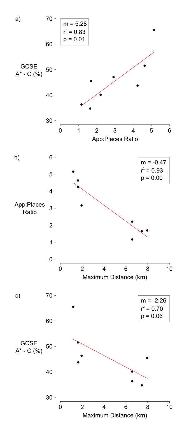
Figure 1. Empirical school-level relationships for schools in Barking and Dagenham 2007–2011. For each plot m = regression coefficient, p = p-value of regression, r2 = coefficient of determination. - 2.4
- These empirical patterns highlight the importance of the location where parents live for the chances of getting their child into popular, generally higher performing, schools. However, interviews with parents in East London have shown a range of attitudes towards the importance of education, from largely indifferent to being the highest priority (Butler and Hamnett 2011). For example, contrast the following two statements from two parents in the same area of East London:
"I think [education is] reasonably important. I wouldn't put it up there as really top ranked just because, you know, I think there's more important things in a child's life." (Butler and Hamnett 2011, p.105)
"Oh, the single most important thing that a parent can give to their children in life is a first-class education" (Butler and Hamnett 2011, p.98).
- 2.5
- With the intention of producing a simple, abstract agent-based simulation model that can generate the general empirical patterns described above, we focus on the over-arching concept of parental 'aspiration' to send a child to the best performing school (measured by exam results). We use the model to represent a range of 'aspiration' regarding educational attainment, from largely indifferent to high priority. Furthermore, we use this notional measure of aspiration as a means to constrain the location and movement of parents within a modelled environment. We examine different mechanisms (i.e., model rule sets) to identify how they influence generated patterns and examine the sensitivity of several key model variables. First we describe the general model structure, before then presenting results and analysis of the different model rule- and parameter sets.
Model Structure
- 3.1
- Our description of model structure uses selected parts of the Overview, Design concepts, and Details (ODD) protocol. The full ODD description can be found online with the model code at openABM.org[3].
Purpose
- 3.2
- The purpose of this model is to investigate mechanisms underlying the geography of educational inequality in the UK and the consequences of these mechanisms for individuals with varying attributes and mobility.
Entities, state variables and scales
- 3.3
- Two types of agents are represented; parents and schools. One iteration of the model is assumed to be equivalent to a single year. Although parents and schools have explicit spatial locations, no space scales are implied or assumed and the model environment is a torus. A torus is appropriate in our simple, abstract model to suppress boundary effects so that observed variation in attainment and access to schools can reliably be attributed to straight-line distances between schools and parents (similar to approaches used in urban segregation models; e.g., Laurie and Jaggi 2003, Fossett and Dietrich 2009). The most important parent attribute is their aspiration to send their child to the best performing school. Aspiration takes a value from 1 to 100 and varies between parents. This range of values represents variation in parents' attitudes towards whether educational attainment (in terms of GCSEs) is the primary criteria for selecting a school (high values) or a less important criteria in selecting a school (low values). It reflects how some parents will seek to maximise the possibility of their child attaining high grades whereas other will be satisfied with less (in the light of other priorities not represented in this model). Parents' aspiration values are set when the parent is created and do not change through time. Parents are assumed to have a single child (not represented as an individual agent, but implicitly as an attribute of the parent). Each parent has two child attributes; child-age and child-attainment. Child-age is measured in years and child-attainment takes a value from 1 to 100. Both child-age and child-attainment change through time. Initially, parents' child-attainment is equal to their aspiration and child-age has a value of 9. Parents have an explicit and unique location (i.e., parents cannot share a location with other parents or a school). Parents can potentially change location once through time.
- 3.4
- Schools have a finite number of places available for allocation to parents each year. Schools have five academic year cohorts (i.e., grades) of parents (pupils) and have a GCSE-score attribute which is calculated as the mean of child-attainment values of parents with child-age = 15 allocated to the school (i.e., GCSE-receiving final-year students[4]). GCSE-score can take a value from 0 to 100. As both allocated parents and child-attainment can change through time, so GCSE-score can vary between schools and through time. Schools have a value-added attribute which is assigned at model initialization and can vary between schools but does not change through time. Value-added can take a value between 0.0 and 1.0. Each year schools record the parents allocated a place and the parents which applied to the school. Schools have an explicit and unique location which cannot change through time. School locations can be random across the model environment, or with equal distance between each school (i.e., on a grid).
Process Overview and scheduling
- 3.5
- Each year existing parents in the environment increase their child-age by a value of 1. School academic year cohorts are also aged (e.g., year 8 parents become year 9 parents) and parents allocated a school place in the previous year (when their child was age 10, now age 11) become year 7. After this increase, parents with child-age = 16 are removed from the model environment, as their children are assumed to have received their GCSEs and left school. This assumption represents the fact that households that no longer have children at school will not be competing for places at schools (and not be occupying places at those schools) and ensures space is available in the environment for parents with younger children applying for school places. Creating this space is important so that the reproduction of educational inequality can be examined through time and shares similarities with similarly simple, abstract models of residential segregation that assume a fixed percentage of agents leave the model environment in a given timestep (e.g., Portugali 2000; O'Sullivan 2009).
- 3.6
- New parents are then added to the model environment. The number of new parents added is given by Families * Number-of-Schools. The values of these variables are specified by the user at model initialization and do not change through time. New parents are assigned to unoccupied locations in the model environment. Location assignment can be spatially random or constrained by aspiration. If constrained, the mean aspiration of parents in the Moore neighbourhood (i.e., 8 surrounding locations) of each unoccupied location is calculated (known as location-value; if a given location has no parents in its Moore neighbourhood its location-value is set to the mean aspiration of all parents in the model environment). New parents are assigned the unoccupied location with greatest location-value which is also less than that parent's aspiration. If no location matches these criteria (i.e., all unoccupied locations have location-value > new parent aspiration) the new parent is assigned the location with the smallest location-value.
- 3.7
- Parents which have not yet been allocated a school (i.e., those with child-age = 9 or child-age = 10) then assess schools. These parents assess whether they believe they are within the 'catchment' of each school. Each year the mean spatial distance of all allocated parents at a school is calculated. Parents assume they are in a school catchment if their distance to the school is less than the smallest mean distance for the last parent-memory years. The parent-memory parameter is set by the user at model initialization, does not vary in time or between parents, and can take a value from 1 to 5. Unallocated parents also assess which school they consider satisfactory to send their child to. Satisfactory schools are those with:

(1) Finally, these unallocated parents assess which 'poor' schools they want to avoid sending their child. These schools to be avoided are those with:

(2) The avoided-threshold parameter is a global parameter which does not vary in time or between parents and can take a value from 0 to 1.
- 3.8
- Parents with child-age = 9 (i.e., one year before they will be allocated to a school) then check if they want to move from their current location to try to increase their chance of having their child allocated to a satisfactory school (in the next year) by living closer to that school. Parents rank the top Number-of-Rank schools using one of eight strategies, depending on their circumstances (see Table 1). They then check locations in catchments of these schools in rank order (starting with top rank) until a location is found or all school catchments have been checked. Parents will not be able to move if there are no unoccupied locations in a catchment or if availability of locations is constrained by location-value (see above). The year in which a child-age = 9 is the only one in which parents can move. Ultimately, this is not an accurate representation of reality as parents could move multiple times before and after school allocation. However, this single-move assumption is credible given that aspects that may influence house moves other than schooling (e.g., changes in family income or size) are not represented in this simple, abstract model.
Table 1: Idealised parent ranking strategies for moving. Schools considered by parents to be satisfactory or to be avoided are determined by Eq. 1 and Eq. 2, respectively. Strategy Criteria Response 1 Believed to be in no school catchment No schools considered satisfactory No schools avoided Rank all schools by GCSE-score descending 2 Believed to be in no school catchment
No schools considered satisfactory
At least one school avoidedRank all schools – except those avoided – by GCSE-score descending 3 Believed to be in no school catchment
At least one school considered satisfactory
No schools avoidedRank schools considered satisfactory by GCSE score descending, then all other schools by GCSE score descending 4 Believed to be in no school catchment
At least one school considered satisfactory
At least one school avoidedRank schools considered satisfactory by GCSE score descending, then all other schools – except those avoided – by GCSE score descending 5 Believed to be in one or more school catchment
No schools considered satisfactory
No schools avoidedRank schools considered satisfactory by GCSE score descending, then all other schools by GCSE score descending 6 Believed to be in at least one school catchment
No schools considered satisfactory
At least one school avoidedRank schools considered satisfactory by GCSE score descending, then all other schools – except those avoided – by GCSE score descending 7 Believed to be in at least one school catchment
At least one school considered satisfactory
No schools avoidedDo not try to move 8 Believed to be in at least one school catchment
At least one school considered satisfactory
At least one school avoidedRank schools considered satisfactory by GCSE score descending, then all other schools – except those avoided – by GCSE score descending - 3.9
- Parents with child-age = 10 rank the top Number-of-Rank schools that they will apply to send their child to using one of eight strategies depending on their circumstances (see Table 2). To determine which strategy to use, parents check which school catchment(s) they believe they are located within and whether there are schools they deem satisfactory to send their child[5].
Table 2: Idealised parent ranking strategies for school application. Schools considered by parents to be satisfactory or to be avoided are determined by Eq. 1 and Eq. 2, respectively. Strategy Criteria Response 1 Believed to be in no school catchment No schools considered satisfactory No schools avoided Rank all schools by distance ascending 2 Believed to be in no school catchment
No schools considered satisfactory
At least one school avoidedRank all schools – except those avoided – by distance ascending 3 Believed to be in no school catchment
At least one school considered satisfactory
No schools avoidedRank schools considered satisfactory by distance ascending, then all other schools by distance ascending 4 Believed to be in no school catchment
At least one school considered satisfactory
At least one school avoidedRank schools considered satisfactory by distance ascending, then all other schools – except those avoided – by distance ascending 5 Believed to be in one or more school catchment
No schools considered satisfactory
No schools avoidedRank those schools believed to be in the catchment of by GCSE score descending, then all other schools by distance ascending 6 Believed to be in at least one school catchment
No schools considered satisfactory
At least one school avoidedExcept for those schools avoided, rank schools believed to be in the catchment of by GCSE score descending followed by all other schools by distance ascending 7 Believed to be in at least one school catchment
At least one school considered satisfactory
No schools avoidedRank those schools believed to be in the catchment of by GCSE score descending, then those schools considered satisfactory by distance ascending, then all others schools by distance ascending 8 Believed to be in at least one school catchment
At least one school considered satisfactory
At least one school avoidedExcept for those schools avoided, rank those schools believed to be in the catchment of by GCSE score descending, then those schools considered satisfactory by distance ascending, then all other (non-avoided) schools by distance ascending - 3.10
- Schools then allocate places[6] to parents with child-age = 10 ready for their child to become a pupil of the school the next year. Schools allocate applicants that ranked them highest first (starting with the closest parent and allocating in ascending order of distance). Once all schools have allocated these top-ranking parents, if places remain unallocated (i.e., if there were less parents ranking them first than total places available) schools then allocate applicants that ranked them second (again, allocating by distance ascending). This process continues (third ranks, fourth ranks, etc.) until all parents' rankings have been checked. Schools that have remaining places after all ranked preferences have been allocated, then allocate remaining places to unallocated parents on distance (closest allocated first then by distance ascending). This approach to school-place allocation implements the Gale-Shapley (1962) method (with ranking determined by distance to school) as used by LEAs in England (Allen et al. 2010).
- 3.11
- Finally, also in preparation for the following year, existing parents already allocated a place at a school update their child-attainment using the idealised relationship:
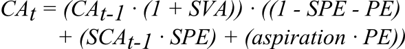
(3) where CA is child-attainment, SVA is the value-added of the school attended, SPE is School-Peer-Effect, PE is Parent-Effect, SCA is the mean child-attainment of all parents allocated a place at the school and t denotes the timestep. Multiple factors are believed to influence changes in pupil attainment during their time at secondary school, attributable to individual pupils' backgrounds (e.g., ethnicity and class; Connolly 2006; Hamnett et al. 2007) and school-level factors (e.g., school composition and peer-effects; Thrupp et al. 2002; Willms 2010). The structure and composition of Eq. 3 allows the relative importance of several factors to be examined. Specifically, School-Peer-Effect and Parent-Effect can take values from 0 (no effect on pupil attainment through time) to 0.5 (large effect on pupil attainment through time) and reflect the influence of the attainment of pupils' peers and the aspirations of their pupils' parents on attainment. The possible influence of factors beyond pupils and parents themselves (i.e., facilities, teachers etc of the school itself) is reflected by value-added. When each of these three variables is zero there is no change in pupil attainment through time. Schools then update their GCSE-score to be the mean of child-attainment of allocated parents with child-age = 15 (i.e., year 11 pupils).
Model Testing and Evaluation
-
State Variables
- 4.1
- To evaluate and test the model we consider state variables at three different levels of aggregation and scale. To measure spatial autocorrelation of parent aspiration at the level of the entire simulated environment we use Moran's I, calculating the statistic and the probability that the statistic is statistically significantly different from zero (p) for each timestep. We cannot estimate Moran's I for empirical data and so do not consider this an empirical pattern by which to assess the generative properties of the model rules. However, this measure is a useful means to identify if local interactions rules result in system-level spatial patterns (i.e., spatial autocorrelation of parent agent attributes). At the school level we measure GCSE-score (corresponding to GCSE-5+), A:P and MaxDist and fit linear regression models (with coefficient and significance values m and p, respectively) and calculate the coefficient of determination (r2) for each combination of pairs of these variables in each timestep (as we did for empirical data in Figure 1). For regression models from model output we calculate the mean model coefficient, mean r2 and the mean number of timesteps during a model run in which regression p > 0.05. We use values for m, p and r2 as indicators to compare how results for different model rules sets reproduce the general patterns outlined above, using the quantified values for our empirical regressions as a guide. Thus, we assume that model results with larger absolute values of m, higher r2 values and lower p values indicate stronger reproduction of general empirical patterns. At the parent level we consider parent strategy for school application (see Table 2), application success, distance to allocated school, aspiration, child-attainment change, and whether the parent moved or not prior to allocation. Parent application success is evaluated by comparing whether a child was allocated a place at their top ranked school (success if so, otherwise not). Change in child-attainment is the difference between child-attainment when child-age = 10 (i.e., prior to entering school) and when child-age = 15 (i.e., when receiving GCSE results and leaving school). We do not currently have empirical equivalents with which to compare these measures.
Methods
- 4.2
- To test and evaluate the model we consider which model rules and/or conditions are necessary for the model to generate the school-level empirical patterns described above (Section 2). Hence, the approach is 'generative' (Epstein 1999). We also examine how different rules and model conditions influence spatial autocorrelation of parent aspiration across the entire model environment. We evaluate the importance of the spatial distribution of schools, location constraints, and school value-added (Table 3). We evaluate the importance of three model rule options: i) the spatial distribution of schools, by either locating them randomly across the model environment or regularly spaced (on a grid); ii) the importance of parental location constraints, by running the model with and without the constraint of location-value; and iii) the importance of school value-added, by either setting all schools' value-added to zero or allowing values to vary randomly (between 0 and 1). For each of the eight rule-sets the combinations of these rule options produce (Table 3), we run the model 25 times for 100 timesteps (with parameter values as shown in Table 4). For analysis we use only the last 80 timesteps of each model run as random initialization means that it takes at least 10 timesteps before schools have had a single cohort of students pass through the school with child-attainment correctly calculated (Eq. 3, and see initial variation in variables in Figure 2).
Table 3: Combinations of rules for model testing. Rule Set Random Schools Location Constraints School Value-Added 1 No Yes Yes 2 No No Yes 3 Yes Yes Yes 4 Yes No Yes 5 No Yes No 6 No No No 7 Yes Yes No 8 Yes No No Table 4: Default parameter values used in model runs (unless otherwise specified). Parameter Value Families 100 Parent-Memory 5 Number-of-Schools 9 Number-of-Ranks 4 Initial-School-GCSE-Distribution Uniform, 1 Parent-Aspiration-Distribution Gaussian, μ = 50 σ = 20 Aspiration-Mean 50 School-Value-Added-Distribution Gaussian, μ = 0 σ = 0.1 Avoided-Threshold 0.5 School-Peer-Effect 0.25 Parent-Effect 0.25 - 4.3
- For the model that best generates empirical patterns we also perform sensitivity analyses (for parameters and values as shown in Table 5).
Table 5: Parameter values used in sensitivity analyses. Parameter Set Parameter Value 9 Number of Ranks 2 10 Number of Ranks 6 11 Avoided Threshold 0.05 12 Avoided Threshold 0.25 13 Avoided Threshold 0.75 14 Avoided Threshold 0.95 15 School Peer Effect, Parent Effect 0.00, 0.00 16 School Peer Effect, Parent Effect 0.25, 0.00 17 School Peer Effect, Parent Effect 0.50, 0.00 18 School Peer Effect, Parent Effect 0.00, 0.25 19 School Peer Effect, Parent Effect 0.50, 0.25 20 School Peer Effect, Parent Effect 0.00, 0.50 21 School Peer Effect, Parent Effect 0.25, 0.50 22 School Peer Effect, Parent Effect 0.50, 0.50 Results: Rule sets
- 4.4
- Relationships between state variables (Table 6) indicate that the model produces results which generate empirical patterns most closely and consistently (i.e., large m, high r2, low p) when parents are constrained by where they can live, when schools differentially add value to pupils' attainment and when schools are not randomly located (i.e., Rule Set 1, Table 3). Results indicate that at least one of the Location Constraints or School Value-Added rules is needed to generate the relationship between school performance and popularity (GCSE-5+ vs. A:P). If neither is present (e.g., Rule Sets 6 and 8), the range of school performance is very low (i.e., little difference between maximum and minimum school GCSE-5+, Figure 2), and therefore no clear preferences between schools arise. To generate strong spatial autocorrelation in parent aspiration the Location Constraints rule is needed (Rule Sets 1, 3, 5, 7) as these constraints produce 'neighbourhoods' of aspiration (e.g., Figure 3). In turn, when combined with non-random location of schools (i.e., Rule Sets 1 and 5), constraining the location of parents generates good relationships at school level. Thus, pattern in both location of parents and schools is required to generate empirical relationships, and this is enhanced when schools differ in the value they add to pupils' attainment.
Table 6: Measures of relationships between key empirical variables for different model rule sets[7] Rule GCSE-5+ vs A:P GCSE-5+ vs MaxDist A:P vs MaxDist Moran's I Set m r2 p m r2 p m r2 p Stat. p 1 7.89 0.96 0.00 -0.78 0.70 5.58 -0.09 0.65 10.00 0.92 0.00 2 6.88 0.85 0.68 -0.18 0.38 47.20 -0.02 0.36 50.92 0.01 32.50 3 8.53 0.94 0.12 -0.41 0.23 70.16 -0.04 0.20 71.16 0.91 0.00 4 6.51 0.76 4.84 -0.01 0.13 74.68 0.00 0.14 74.44 0.01 31.50 5 6.98 0.97 0.00 -0.67 0.68 8.60 -0.09 0.65 10.96 0.92 0.00 6 1.79 0.30 56.68 0.00 0.12 76.16 0.00 0.11 76.88 0.01 46.00 7 7.36 0.92 2.60 -0.26 0.18 71.92 -0.03 0.16 74.96 0.91 0.00 8 1.37 0.26 61.40 0.01 0.15 74.44 0.00 0.17 72.56 0.01 54.00 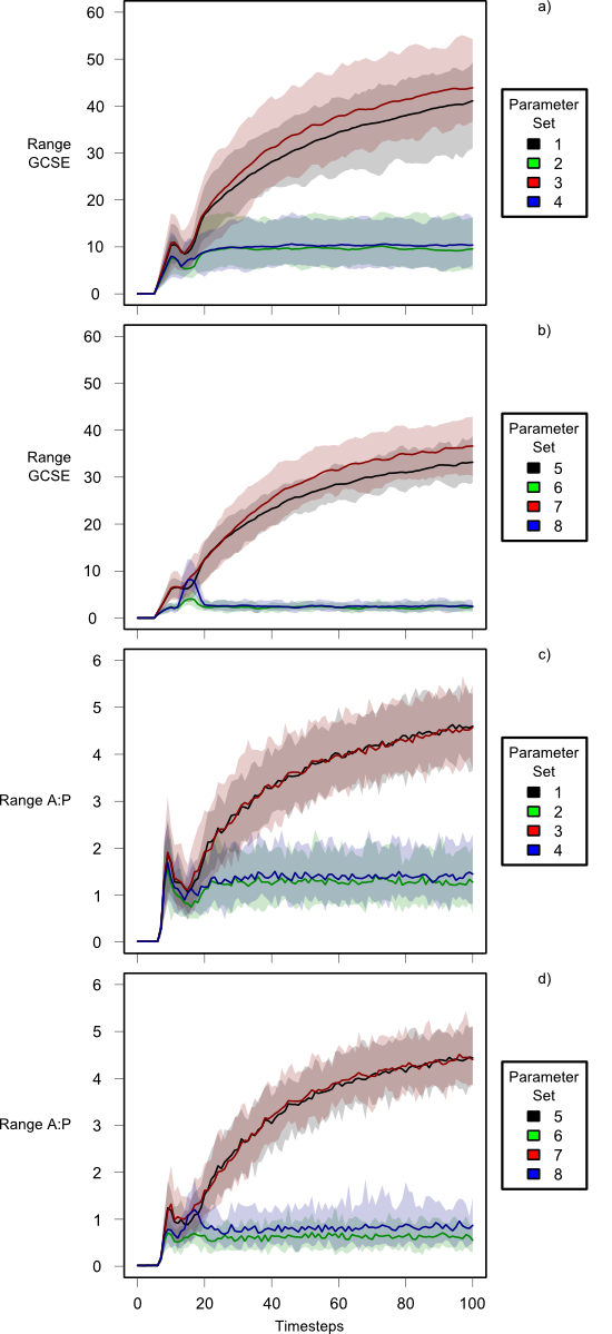
Figure 2. Time series of GCSE and range and A:P range. Solid lines are the mean of 25 model runs for the given parameter set. Shaded areas are the 95% confidence interval around the corresponding mean, calculated from the standard error of 25 model runs. 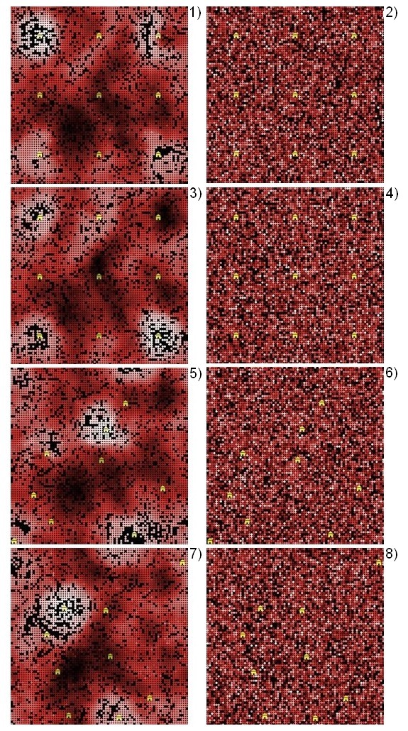
Figure 3. Example final model state maps. Maps are of parent aspiration (lighter shades are higher aspiration). Schools are shown as house icons (lighter shades indicate higher GCSE-score). Numbers indicate Rule Sets (as summarised in Table 3). Results: Sensitivity analysis
- 4.5
- When compared to results for the best model rule set (Rule Set 1), sensitivity analysis results indicate that modelled school-level relationships are largely insensitive to variation in parameters influencing parents' school ranking and child-attainment change (Table 7). The exception is for higher values of avoided-threshold (Eq. 2). When avoided-threshold = 0.95 (Parameter Set 6) relationships between GCSE-5+ and MaxDist and between A:P and MaxDist break down (i.e., there is no relationship) and for avoided-threshold = 0.75 (Parameter Set 5) the relationships become weaker (i.e., no relationship more frequently).
Table 7: Measures of relationships between key empirical variables for sensitivity analyses[8] Parm GCSE-5+ vs A:P GCSE-5+ vs MaxDist A:P vs MaxDist Moran's I Set m r2 p m r2 p m r2 p Stat. p 1 11.21 0.93 0.00 -0.70 0.65 8.76 -0.06 0.61 12.16 0.93 0.00 2 7.66 0.90 0.00 -0.79 0.69 6.08 -0.09 0.60 12.68 0.91 0.00 3 8.35 0.96 0.00 -0.80 0.71 5.00 -0.09 0.67 8.04 0.92 0.00 4 8.09 0.96 0.00 -0.80 0.70 4.12 -0.09 0.66 7.08 0.92 0.00 5 5.39 0.93 0.04 -0.68 0.59 20.56 -0.11 0.53 25.80 0.92 0.00 6 6.12 0.88 0.40 -0.04 0.13 76.52 0.00 0.11 78.12 0.93 0.00 7 9.67 0.95 0.00 -1.06 0.69 7.60 -0.11 0.67 9.12 0.92 0.00 8 10.69 0.93 0.00 -1.18 0.71 5.64 -0.11 0.69 6.44 0.92 0.00 9 10.80 0.93 0.00 -1.13 0.68 9.60 -0.10 0.66 12.40 0.92 0.00 10 8.11 0.95 0.00 -0.84 0.70 5.52 -0.10 0.65 10.28 0.92 0.00 11 7.39 0.96 0.00 -0.71 0.68 7.76 -0.09 0.63 12.32 0.92 0.00 12 7.37 0.96 0.00 -0.72 0.64 10.16 -0.09 0.60 17.76 0.91 0.00 13 7.16 0.96 0.00 -0.68 0.67 8.28 -0.09 0.63 12.92 0.91 0.00 14 7.04 0.97 0.00 -0.66 0.66 9.72 -0.09 0.62 13.12 0.92 0.00 Results: Parent-level analysis
- 4.6
- At the parent level, plots of proportions of parents in classes of one state variables against classes of other state variables are useful to identify relationships between those variables (e.g., Figure 4). Some of these relationships are appropriate for verifying model function given model structure, but others are interesting to understand what the model structure implies for parents with different attributes.
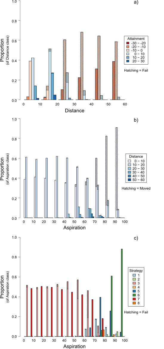
Figure 4. Relationships between variables at the parent-level of analysis (for Rule Set 1). - 4.7
- As expected, given distance-based school allocation rules in the model, results show that parents living closer to their allocated school are more likely to have ranked that school as their top preference (Figure 4a). Furthermore, of parents that successfully get their child into their top ranked school, more have positive child-attainment change (blue colours in Figure 4a) than negative (red colours). However, it is not the parents in the closest distance class (distance < 10) that have greatest positive child-attainment change. Rather, on average it is parents in the second distance class (10–20) that achieve greatest child-attainment increases. For example, a greater proportion of parents in the second distance class have positive child-attainment than those in the closest (82% compared with 56%) and overall mean child-attainment change is greater for the second class (+6.36) than the closest (+1.76). In contrast, the vast majority (92%) of parents in the fourth distance class and greater (i.e., allocated distance ≥ 30) have negative child-attainment change. Of parents in these distance classes, only 1% were successful in getting their child into their top-ranked school, again highlighting the importance of distance allocation rules and their relationship with school (and pupil) performance.
- 4.8
- When we consider relationships between parent aspiration, allocated distance and whether parents have moved or not (Figure 4b) we observe that as aspiration increases parents are more likely to move. Parents that move are more likely to live in the closest allocated school distance class (distance < 10). No parents in the farthest allocated school distance classes (i.e., distance ≥ 30) moved to be in that position, and these parents are not those with lowest aspiration. Rather, parents with higher than average, but not very high, aspiration (i.e., those with aspiration 60–70) are most likely to be allocated to a school with distance ≥ 30.
- 4.9
- Parents in this medium-high aspiration class (aspiration 60–70) also fail to get their child into their preferred school more often than parents in other aspiration classes (Figure 4c). Parents with aspiration ≥ 70 are more likely to be in a school catchment when applying to a school (Figure 4c, increased proportions of strategies 5–8 in these classes). Furthermore, as aspiration increases, the likelihood of succeeding using strategy 3 to rank schools for allocation decreases (Figure 4c; i.e., the danger of not being in the school catchment of a satisfactory school is greater for those with higher aspiration).
Discussion
-
Model Structure
- 5.1
- Our model testing and evaluation shows how differences between schools' performance (and therefore parents' school preferences) combined with distance-based school-place allocation rules, are needed to reproduce empirically observed school-level patterns. The approach we have used is 'generative' (Epstein 1999, 2006), seeking to explain the emergence of macroscopic (societal) regularities arising from the local interaction of simulated heterogeneous, autonomous agents. Using an agent-based simulation model we have generated observed macroscopic regularities (i.e., relationships between school performance, popularity and allocation) from the 'bottom up' by simulating individual parents' aspirations regarding educational attainment and their efforts to do so in the face of distance-based school allocation rules.
- 5.2
- Starting with random locations of parents and schools with identical performance (GCSE-5+), this generative approach allows us to show that either i) differences in the abilities of parents to move to locations near preferred schools, or ii) variation in the increases in attainment schools can provide to pupils are needed to generate the empirical relationship between school exam (GCSE) performance and school popularity. If neither of these rules is present in the model, variation in school performance is not produced (Figure 2) meaning that parents' school preferences are inconsistent across the modelled environment (i.e., it is not clear which schools are better than others). Differences in the abilities of parents to move are important for creating neighbourhoods (groupings) of parents with similar aspiration (Figure 3; Moran's I in Table 6). In turn, these neighbourhoods mean that children with similar initial attainment (because initial child-attainment is equal to parent aspiration) are more likely to attend the same school, reinforcing improvements in school performance (via School-Peer-Effect). Variation in the improvement that schools can contribute to pupils' attainment also produces variation in school performance, but to a lesser degree than the neighbourhoods of aspiration effect. We found that increasing the range of improvement that schools contribute to pupil attainment (i.e., from σ = 0.1 for School-Value-Added-Distribution to σ = 0.5, Table 4) does increase this effect, but still does not produce as consistently significant relationships as for parent location constraints (e.g., p for GCSE-5+ vs. MaxDist of 22.48 compared with 5.58 and 8.60 for Rule Sets 1 and 5 respectively, Table 6).
- 5.3
- Another model rule-set we investigated was the random location of schools (i.e., Rule Set 3, Table 3). When schools are randomly located spatially across the model environment, the empirically-observed distance relationships collapse. This is because of the abilities of parents to move into desired school catchments and because of the agent logic used in the model. With random school locations, schools are often close together and so parents can be located in more than a single school catchment (i.e., school catchments overlap), a situation which doesn't occur when schools are regularly spaced. Consequently, a greater number of parents are in school catchments when it comes to parents ranking for allocation and schools allocating, as shown by greater proportions of parents in distance classes 10–20 and 20–30 using ranking strategy 7 than 3 (compare Figures 5a and 5b). The overlapping of school catchments also means that parents are more likely to succeed in getting their children into their desired schools when farther from them (compare Figures 5a and 5b) as parents near the school may have sent their child to a different, but nearby, school. This situation implies the model is not useful for considering situations where schools are not spaced equally. However, in its current form we would not expect the model to be useful in this situation as parents' ranking logic for moving only considers the single best school (and its catchment) and does not take account of which locations in the environment would allow them to be in multiple (good) school catchments. Consequently, as the model logic currently stands, the model is best used with regularly spaced schools so that parents are very unlikely to be in more than one school catchment, as the agent logic assumes.
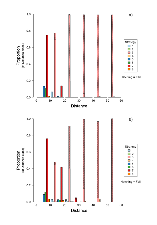
Figure 5. Relationship between distance and strategy at parent-level for randomly located schools for a) Rule Set 1 and b) Rule Set 3 (specified in Table 3). - 5.4
- Also in the current model structure, three mechanisms exist whereby feedbacks between aspiration and child-attainment can occur. These are the assumptions that:
- initial child-attainment is equal to the aspiration of the parents (Att=Asp);
- through time at school child-attainment is influenced by the aspiration of the parent (PE in Eq 3); and
- through time at school child-attainment is influenced by the mean child-attainment of school peers (SPE in Eq 3).
- 5.5
- To check the importance of these assumptions for the generation of the school-level empirical relationships (e.g., Figure 1), we ran the model for the different combinations of these assumptions being present in the model or not (see Table 8, while maintaining other assumptions of Rule Set 1[9]). These tests indicate that if the Att=Asp assumption is absent, the model does not generate the school-level empirical relationships when PE is also not present (i.e., Rule Sets 10 and 12), but performs better when PE is present (i.e., Rule Sets 14 and 15). Furthermore, the SPE effect seems to be the least important of the three assumptions highlighted above, as when this assumptions is absent but the other two assumptions are present school-level relationships are not affected (i.e., compare results for Rule Set 13 with Rule Set 1). Neighbourhoods of aspiration are produced in all combinations of assumptions (indicated by high Moran's I values). These results make sense as although parents of similar aspiration still cluster together, if there is no link between parent aspiration and child-attainment (via either Att=Asp or PE) little variation in school performance is produced by spatial variation in parent aspiration. Although the Att=Asp assumption is useful, these results imply that a perfect correlation between aspiration and initial child-attainment is not necessary for the model to generate empirical relationships.
Table 8: Measures of relationships between key empirical variables for aspiration and child-attainment mechanisms. Rule Set PE SPE Att=Asp GCSE-5+ vs A:P GCSE-5+ vs MaxDist A:P vs MaxDist Moran's I r2 p r2 p r2 p Stat. p 9 F F T 0.93 0.00 0.60 17.24 0.59 17.68 0.93 0.00 10 F F F 0.90 0.00 0.42 39.52 0.41 43.80 0.92 0.00 11 F T T 0.93 0.00 0.61 17.36 0.61 16.76 0.93 0.00 12 F T F 0.88 0.00 0.44 38.12 0.46 37.36 0.93 0.00 13 T F T 0.95 0.00 0.70 5.52 0.67 8.48 0.92 0.00 14 T F F 0.94 0.00 0.67 11.48 0.64 14.60 0.92 0.00 15 T T F 0.94 0.00 0.68 10.48 0.65 13.88 0.92 0.00 Parent-level patterns
- 5.6
- Our generative approach to modelling has shown that the consequences of our assumptions about the system at the individual, parent, level can generate the empirically observed relationships and patterns at the higher, school, level. Although this model is a highly simplified conceptualisation, it allows us to examine relationships between entities at the lower level and between upper and lower levels that would not be possible (or at the least, very difficult) in the real world. For example, our parent-level results (for Rule Set 1, Table 3) show that in general those in the second distance class (distance 10–20) achieve greatest child-attainment increases, and not those in the closest distance class (distance < 10, Figure 4a). This is because those parents that live in the closest distance class have on average greater aspiration than those in the second distance class and therefore have greatest child-attainment initially. Consequently, the child-attainment of these closest parents is on average more likely to decrease than increase.
- 5.7
- Another interesting finding from our parent-level analysis is that those parents with aspiration 60–70 fail to get their child into their preferred school more often than other parents (closely followed by those with aspiration 50–60, Figure 4c). As noted in the results, the likelihood of failing to get into a preferred school using strategy 3 (rank schools considered satisfactory by distance ascending, then all other schools by distance ascending, Table 2) increases as aspiration increases (Figure 4c). Although a greater proportion of parents with aspiration 70–80 fail when using strategy 3 compared to parents with aspiration 60–70, parents in this lower aspiration class have a greater proportion of parents using this strategy overall (parents with higher aspiration are more likely to be in a school catchment and therefore use strategies 5–8). Parents with aspiration 60–70 are no less likely to find themselves outside a school catchment than parents with lower aspiration (Figure 4c) but because their aspiration is higher they consider only better schools satisfactory for their child. This means they have fewer schools to rank (so distance to those schools is likely to be greater), and each of those schools is more likely to have greater numbers of parents deeming them satisfactory to send their child to (and so these schools have many parents ranking them as most preferred). In contrast, parents with lower aspiration (e.g., aspiration < 50) are more likely to get into their preferred school even though not in any school's catchment, both because the distance to the nearest school is likely to be smaller (because there are more schools deemed satisfactory) and because there are fewer other applicants ranking that school as most preferred (because other parents are more likely to avoid it). The failure of parents with aspiration 60–70 to get into their preferred (i.e., top ranked) school is reflected in their greater allocation distances than any other aspiration class (Figure 4b). Furthermore, only approximately 3% of parents with aspiration 60–70 move, and many remain stuck in the position of having higher than average aspiration but not being 'in the right place' (spatially) when they initially arrive in the model environment (because of location constraints). These parents have aspirations 'too high' relative to their ability to move into preferred school catchments.
- 5.8
- The question then arises; how might school allocation rules or policies be modified to help those parents with above average, but not very high, aspiration (and therefore mobility) get into better schools (or at least schools they want)? One way might be to increase the standards of schools so that a greater number meet the aspirations of parents. In so doing, the number of schools that parents with above average but not very high aspiration deem satisfactory to send their child to will increase and the danger of not being in a school catchment should decrease. To investigate this we examine a scenario in which we run the model as for Rule Set 1 (Table 3) but with a greater mean school value-added of 0.2 (although with the same standard deviation as previously of 0.1). Results for this 'improved school standards' scenario indicate that increased ability of schools to raise child-attainment produces changes in strategies for parents with higher aspiration and decreases the proportion of parents with aspiration 60–70 that fail to get their child into their preferred school (Figure 6, compare to Figure 4c). Furthermore, this increase in mean school value-added increases the proportions of parents in other aspiration classes that fail to get their child into a preferred school, resulting in a more even distribution of failure across the aspiration classes.
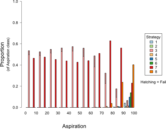
Figure 6. Relationship between aspiration and strategy at parent-level for 'improved school standards' scenario. Prospects for future work
- 5.9
- The 'improved school standards' scenario is just one example of the kinds of scenarios we can examine with the model. The model could also be used to explore alternative school allocation rules and policies, which might include random lotteries for school allocation (e.g., Allen et al. 2013), opening 'free' schools that may use aptitude as a selection criterion (e.g., Hatcher 2011), or the closure of under-performing schools. Future changes to the model might extend it to enable representation of other criteria used in UK state school allocation (e.g., religious faith, attendance of siblings).
- 5.10
- The model presented here uses only a single parent agent variable (aspiration for high educational attainment) to simultaneously represent the goals of parents and the constraints on their ability to meet those goals. However, there are many factors underlying where families want and/or are able to live and which schools they perceive as desirable for their child to attend. For example, educational aspiration varies by class and ethnicity (Butler and Hamnett 2011, 2012) and the ability to move house to achieve these aspirations is an economic question influenced by the housing market. The representation of agents and their environment with multiple attributes that more accurately reflect motivations and constraints is needed. There is no reason why aspiration for educational attainment and economic wealth should be correlated and future modelling may explore how variations in distributions of these factors result in different winners and losers through time and across space. Improving this representation will require individual-level data on attributes, preferences and allocations. These improvements in representation and data would also allow an investigation of motivations for school choice beyond exam results alone, allowing agents to identify preferences based upon school ethnic and socio-economic composition and the attributes of other parents that send their child to a school (although that is in some ways represented here through the Att=Asp assumption).
- 5.11
- What we have been able to show here using a simple, abstract agent-based model that represents individual parents in disaggregated manner, and which was not immediately apparent at the outset, is how constraints on individuals' movements, when combined with distance allocation rules, produce winners and losers that are not directly correlated to the individuals' attributes. That is, it is not agents with lowest aspiration that are least satisfied with their school allocation outcomes, and instead it is parent agents with above average, but not very high, aspiration that fail to get their child into their preferred school more frequently than other parents. Using disaggregated, agent-based simulation approaches like this allows investigation of individual-level outcomes of system level policies. When informed more directly by individual-level data, and used in combination with scenarios of different education policies, this modelling approach will allow us to more rigorously investigate the consequences of those policies for education inequalities across space and through time.
Acknowledgements
- JM is grateful to the Leverhulme Trust for an Early Career Fellowship held during the time of the research presented here. We are also grateful for the comments from three reviewers which helped to improve the manuscript and to David Demeritt whose ideas initiated this work. TB and CH also wish to acknowledge the support of the Economic and Social Research Council (ESRC) which funded the project 'Gentrification, ethnicity and education in East London' (RES-000-23_0793) as well as the contribution of Professor Richard Webber and Dr Mark Ramsden and Dr Sadiq Mir to the original project which gave rise to the findings that inspired this collaboration with JM.
Notes
-
1 Other criteria such as the attendance of siblings at a school and special educational needs are also considered but influence a very minor proportion of all applicants.
2 Data from: Department for Education. Secondary School GCSE Performance Tables 2010: Barking and Dagenham. HMSO. 2011. URL: http://www.education.gov.uk/schools/performance/archive/schools_10/pdf_10/301.pdf. Accessed: 2012-10-18. (Archived by WebCite® at http://www.webcitation.org/6BVNtJTe9); Department for Education. Secondary School GCSE Performance Tables 2011: Barking and Dagenham. HMSO. 2012. URL: http://www.education.gov.uk/schools/performance/2011/download/pdf/301_ks4.pdf. Accessed: 2012-10-18. (Archived by WebCite® at http://www.webcitation.org/6BVNziv1Z); London Borough of Barking and Dagenham. The Right Secondary School: Information for parents about moving to secondary schools in 2013. London Borough of Barking and Dagenham. 2012. URL: http://www.lbbd.gov.uk/Education/Admissions/Documents/RSS2013.pdf. Accessed: 2012-10-18. (Archived by WebCite® at http://www.webcitation.org/6BVOM2pTi); London Borough of Barking and Dagenham. The Right Secondary School: Information for parents about moving to secondary schools in 2012. London Borough of Barking and Dagenham. 2011. URL: http://www.lbbd.gov.uk/Education/Admissions/Documents/RSS2012.pdf. Accessed: 2012-10-18. (Archived by WebCite® at http://www.webcitation.org/6BVOUK84I)
3 http://www.openabm.org/model/3364/version/1/
4 In real schools, pupils in year 11 may be aged 15 or 16 depending on their birth date. However, the temporal resolution of the model is one year and child ages are updated simultaneously so we assume pupils are aged 11 during school year 7, 12 during year 8, etc. until being age 15 during year 11.
5 Note that ranking strategies for both moving and application include situations in which parents do not consider any schools satisfactory to send their child to. In this unsatisfactory situation in the real world, parents may have the means to move to a location outside their current LEA where they think they their child will get a place at a satisfactory state school. Alternatively, if they have the means they may remove their child from the state school system and send them into private schooling. Neither of these options is represented by the current model structure, which is essentially a closed system.
6 In reality, school places are allocated by the Local Education Authority (LEA) and not by individual schools. However, the school-driven allocation procedure used in the model here is consistent with the logic used by an LEA and does not require the use of ancillary model objects other than schools and parents.
7 In the table m is mean regression coefficient of a linear regression between the two variables, p is the mean number of timesteps in which p > 0.05 for the relationship between the variables, and r2 is the mean coefficient of determination for the linear regression model. All values are for 80 timesteps in 25 model replicates.
8 In the table m is mean regression coefficient of a linear regression between the two variables, p is the mean number of timesteps in which p > 0.05 for the relationship between the variables, and r2 is the mean coefficient of determination for the linear regression model. All values are for 80 timesteps in 25 model replicates.
9 Note that we present only seven combinations, as the combination with all three assumptions true is equivalent to Rule Set 1 in Table 3.
References
-
ALLEN, R. and Vignoles, A. (2007). What should an index of school segregation measure? Oxford Review of Education, 33(5), 643–668. [doi:10.1080/03054980701366306]
ALLEN, R., Burgess, S. and McKenna, L. (2010). The early impact of Brighton and Hove's school admission reforms. Centre for Market and Public Organisation. Working Paper No. 10/244
ALLEN, R., Burgess, S. and McKenna, L. (2013). The short-run impact of using lotteries for school admissions: early results from Brighton and Hove's reforms. Transactions of the Institute of British Geographers 38(1), 149–166. [doi:10.1111/j.1475-5661.2012.00511.x]
BRADLEY, J.E., Kirby, A.M. and Taylor, P.J. (1978). Distance decay and dental decay: A study of dental health among primary school children in Newcastle upon Tyne. Regional Studies, 12(5), 529–540. [doi:10.1080/09595237800185501]
BURGESS, S. and Briggs, A. (2010). School assignment, school choice and social mobility. Economics of Education Review, 29(4), 639–649. [doi:10.1016/j.econedurev.2009.10.011]
BUTLER, T. and Hamnett, C. (2007). The Geography of Education. Urban Studies, 44(7), 1161–74. [doi:10.1080/00420980701329174]
BUTLER, T. and Hamnett, C. (2011). Ethnicity, Class and Aspiration: Understanding London's new East End. The Policy Press, Bristol.
BUTLER, T. and Hamnett, C. (2012). Praying for success? Faith schools and school choice in East London. Geoforum 43(6), 1242–1253. [doi:10.1016/j.geoforum.2012.03.010]
CONNOLLY, P. (2006). The effects of social class and ethnicity on gender differences in GCSE attainment: A secondary analysis of the Youth Cohort Study of England and Wales 1997–2001. British Educational Research Journal, 32(1), 3–21. [doi:10.1080/01411920500401963]
EPSTEIN, J. M. (1999). Agent-based computational models and generative social science. Complexity, 4, 41–60. [doi:10.1002/(SICI)1099-0526(199905/06)4:5<41::AID-CPLX9>3.0.CO;2-F]
EPSTEIN, J.M. (2006). Generative Social Science. Princeton University Press, Princeton.
FOSSETT, M. and Dietrich, D.R. (2009). Effects of city size, shape, and form, and neighborhood size and shape in agent-based models of residential segregation: are Schelling-style preference effects robust? Environment and planning. B, Planning & design, 36(1), 149–169. [doi:10.1068/b33042]
GALE, D. and Shapley, L.S. (1962). College admissions and the stability of marriage. The American Mathematical Monthly, 69(1), 9–15. [doi:10.2307/2312726]
GIBBONS, S. and Telhaj, S. (2007). Are Schools Drifting Apart? Intake Stratification in English Secondary Schools. Urban Studies, 44(7), 1281–1280. [doi:10.1080/00420980701302346]
GUDSON, K. (2011). Education Policy, Space and the City: Markets and the (In)visibility of Race. Routledge, London.
HAMNETT, C., Ramsden, M. and Butler, T. (2007). Social background, ethnicity, school composition and educational attainment in East London. Urban Studies, 44(7), 1255–1280. [doi:10.1080/00420980701302395]
HAMNETT, C. and Butler, T. (2011). 'Geography matters': the role distance plays in reproducing educational inequality in East London. Transactions of the Institute of British Geographers, 36(4), 479–500. [doi:10.1111/j.1475-5661.2011.00444.x]
HARLAND, K. and Heppenstall, A.J. (2012). Using Agent-Based Models for Education Planning: Is the UK Education System Agent Based? In: A.J. Heppenstall Heppenstall, A.T. Crooks, L.M. See, and M. Batty (Eds.), Agent-Based Models of Geographical Systems, (pp. 481–497) Springer. [doi:10.1007/978-90-481-8927-4_23]
HARRIS, R.J. and Johnston, R.J. (2008). Primary schools, markets and choice: studying polarization and the core catchment areas of schools. Applied Spatial Analysis and Policy 1(1), 59–84. [doi:10.1007/s12061-008-9002-8]
HATCHER, R. (2011). The Conservative-Liberal Democrat Coalition government's "free schools" in England. Educational Review, 63(4), 485–503. [doi:10.1080/00131911.2011.616635]
LAURIE, A.J. and Jaggi, N.K. (2003). Role of 'vision' in neighbourhood racial segregation: a variant of the Schelling segregation model. Urban Studies, 40(13), 2687–2704. [doi:10.1080/0042098032000146849]
MAROULIS, S., Guimerà, R., Petry, H., Stringer, M.J., Gomez L.M., Amaral, L.A.N. and Wilensky, U. (2010a). Complex Systems View of Educational Policy Research. Science, 330, 38–89. [doi:10.1126/science.1195153]
MAROULIS, S., Bakshyy, E., Gomez, L. and Wilensky, U. (2010b). An Agent-Based Model of Intra-District Public School Choice. http://ccl.northwestern.edu/papers/choice.pdf. Archived at: http://www.webcitation.org/6BsXYmTOL
MCLAFFERTY, S. (1982). Urban Structure and Geographical Access to Public Services. Annals of the Association of American Geographers, 72(3), 347–354. [doi:10.1111/j.1467-8306.1982.tb01830.x]
MILLINGTON, J.D.A., O'Sullivan, D., Perry, G.L.W. (2012). Model histories: Narrative explanation in generative simulation modelling. Geoforum, 43, 1025–1034. [doi:10.1016/j.geoforum.2012.06.017]
O'SULLIVAN, D. (2008) Geographical information science: agent-based models. Progress in Human Geography, 32, 541–558. [doi:10.1177/0309132507086879]
O'SULLIVAN, D. (2009). Changing Neighborhoods—Neighborhoods Changing A Framework for Spatially Explicit Agent-Based Models of Social Systems. Sociological Methods & Research, 37(4), 498–530. [doi:10.1177/0049124109334793]
PORTUGALI, J. (2000). Self-organization and the city. Springer. [doi:10.1007/978-3-662-04099-7]
SIMINI, F., González, M.C., Maritan, A. and Barabási, A.L. (2012) A universal model for mobility and migration patterns. Nature, 484(7392), 96–100. [doi:10.1038/nature10856]
TANG, Y., Parsons, S. and Sklar, E. (2007) Modeling Human Education Data: From Equation-Based Modeling to Agent-Based Modeling In: Antunes, L. and Takadama, K. (Eds.) MABS 2006, Lecture Notes in Computer Science, 4442 41–56.
THRUPP, M., Lauder, H. and Robinson, T. (2002). School composition and peer effects. International Journal of Educational Research, 37(5), 483–504. [doi:10.1016/S0883-0355(03)00016-8]
WILLMS, J. D. (2010). School composition and contextual effects on student outcomes. The Teachers College Record, 112(4), 3–4.