
 Abstract
- The proliferation of resistant strains has been an unintended side effect of human interventions designed to eliminate unwanted elements of our environment. Any attempt to destroy an adaptive population must also be considered as a selection pressure, so that the most resistant members will comprise the next generation. Procedures have been developed to slow the evolution of resistances in a population, with the most common approaches being overkill and treatment cycling. This paper presents an agent-based Susceptible-Infection-Susceptible (SIS) model to explore the effectiveness of these procedures on an abstract epidemic of pathogens, focusing on how the interaction between interventions and mutations affects acquired resistance. Illustrative findings indicate that overkill performed better than cycling treatments when variation in resistances had a high degree of heritability. When resistance variation was effectively memoryless, cycling and overkill performed comparably. However, overkill was prone to backlash outliers where an amplification of infection resistance occurred- a significant drawback to the overkill technique. These backlash events indicate that cycling interventions might be more effective when variation is memoryless and carrying resistance incurs a cost to overall fitness. However, under limited fitness-cost conditions explored, cycling performed no better than overkill for preventing resistance.
- Keywords:
- Evolution, Acquired Resistance, Agent Based Modeling, Selection Pressure, SIS Model, PS-I
Introduction
- 1.1
- Adaptation is necessary for life - it is literally one of the traits used to define life under conventional definitions (Patten, Straskraba, & Jørgensen 1997; Koshland 2002). This adaptation could be within the lifespan of an organism or part of a genetic selection process. In this light, it is unsurprising that human interventions intended to eliminate unwanted entities are met with acquired resistance. In the presence of inherited traits, this process is almost inevitable: the method meant to destroy pathogens creates a selection pressure that favors resistant varieties. While it is impossible to prevent the emergence of resistant strains, approaches have been proposed to slow the spread of resistance. By slowing the rate that these unwanted elements gain the ability to resist or avoid interventions, each intervention can be used over a longer period of time. This application of agent-based modeling explores the implications of using different intervention strategies to slow the spread of resistant strains. While the model developed in this paper most closely analogues the case of bacterial or viral populations, the fundamental mechanisms are abstract and their insights may apply to other contexts.
- 1.2
- Evolution is the main process that builds population resistance in the domain of biology. Evolution requires three conditions: inheritance, variation, and selection pressure (Darwin 1859). Evolution passes information via vertical transmission, from parents to offspring as opposed to general adaptation which may also include horizontal transmission (communication, imitation). In pathology, scientists have mapped out the basic mechanisms for evolution (Levy & Marshal 2004). Inheritance occurs as a function of genetic copying and transmission during asexual reproduction. Reproduction creates new infected hosts in the local area. Variation exists in the microbial population due to heritable mutations. Selection pressures result from the microbe's environment, the host organism, particularly as a result of antibodies and medical treatments such as antibiotics. Certain variants of pathogens will survive negative selection pressures such as a certain type of antibiotic, displaying resistance to that selection pressure. As a result, research has demonstrated a significant tradeoff between successful treatment and the emergence of resistance to treatments employed (Wang & Lipsitch 2006).
- 1.3
- This research presents an agent-based model to explore tradeoffs between resistance and intervention strategies, including those intended to limit resistance. Rather than focus the model intensively on a single pathogen, this model implements general mechanisms that are shared in common across these problems. By focusing on this problem in an abstract manner, this model can vary mechanisms that are fixed for a given pathogen (e.g., mutation mechanisms). As such, this model works at the intersection of evolutionary game theory with research on pathogens. The purpose of this work is to examine abstract characteristics of these problems, with a particular focus on why an intervention such as overkill (multiple simultaneous treatments) might be superior for some problems, while cycling (alternating treatments) might be superior for others.
Background
- 2.1
- How should an intervention be structured such that the undesirable population does not rebound with a newly fostered resistance? To address this question requires a series of steps: identify where population resistance is a problem, discover successful intervention strategies, and examine why these are effective. Within different fields, a wealth of information exists for the study of interventions that successfully avoided or slowed population resistance. Palumbi's "Humans as the World's Greatest Evolutionary Force" contains a set of effective approaches within the fields of biology and medicine (Palumbi 2001).
- 2.2
- Palumbi's techniques refer not to the use of particular drugs or treatments but to effective courses of treatments over time, which will be referred to as interventions. Under this definition, an intervention is a subset of game theory's concept of strategy, where the game must include multiple stages. Using interventions found to be effective, the next logical step is to identify the factors that support or contraindicate interventions based on their impact in the population adaptation process. The experiments and analysis conducted in this research address this open question.
- 2.3
- Evolution is studied directly in the field of pathology. MRSA (Methicillin Resistant Staphylococcus Aureus) bacteria showcase the impact of a treatment resistant organism on human well being. For fifty years, it was taken for granted that systemic antibiotics could eradicate almost any staph infection. Outbreaks over the last ten years of drug resistant (and multi-drug resistant) strains have exposed the danger of such complacency. Strains of staph exist which resist all commonly used antibiotics, setting the stage for a public health crisis (Klevens et al. 2007). Similar hazards are evident in the field of virus pathology. HIV has been shown to mutate fast enough to resist individual drug treatments within the lifespan of a single patient (Crandall 1999).
- 2.4
- Growing awareness of acquired resistances in MRSA and HIV has driven the study of effective courses of treatments to best combat infections. Interventions such as single treatment, overkill, cycling, and irregular treatments have been examined at both the microbial and public health level (Palumbi 2001). An intervention consisting of a single treatment consists of one treatment, applied until the infection appears to be completely extinguished. Overkill involves multiple treatments applied simultaneously, until no infection remains. Overkill relies on the improbability of an infection adapting to multiple treatments simultaneously. A cycled intervention alternates multiple individual treatments over time. Cycling relies on the principle that a shifting selection pressure will delay or remove the tendency of the pathogen to develop any given resistance. Irregular interventions involve lapses in treatment, where the infection is not eliminated but no treatment is applied. Irregularity is discouraged, as they tend to allow recovery of pathogen populations - potentially with greater resistances.
- 2.5
- Fundamentally, the effectiveness of different strategies (overkill, cycling, etc) depends on mechanisms of reproduction and mutation. To examine these relationships, this work develops and explores a simple agent-based model capable of evolution and acquired resistances. This model is an agent-based implementation of a Susceptibility-Infection-Susceptibility (SIS) epidemiology model. SIS models are well-established for examining infection, recovery, and re-infection by pathogens in a substrate of hosts (Parshani, Carmi, & Havlin 2010). SIS models are frequently applied to examine transmission and population dynamics of pathogens in hosts, often as a function of spatial topography or host traits (Messinger & Ostling 2009; Jiang, Sullivan, Su & Zhao 2011). SIS models have traditionally focused on a single pathogen to complement empirical epidemiological work, rather than competition or evolution of pathogens.
- 2.6
- However, recent work has studied natural competition and evolution of pathogens using SIS and similar epidemiological models. Kerr, Neuhauser, Bohannan & Dean (2006) used a cellular automata examine the effects of spatial migration boundaries on competing viral pathogen strains in a population of bacterial hosts. Wang, Jin, & Liu (2011) compared evolutionary dynamics, extinction, and co-existence between a spatial (automata lattice) and non-spatial (dynamical) SIS model. The spatial model of Wang et al. (2011) is most similar to the model designed in this work, with related goals to examine the evolution of competing pathogen strains. However, despite their extensive focus, spatial aspects are only one factor influencing pathogen dynamics.
- 2.7
- The primary addition of this work over prior work with SIS models is the examination of the interaction between acquired resistance and intervention strategies. Prior SIS models were not designed to examine this relationship in detail: models of pathogen competition and evolution have focused primarily on virulence, rather than resistance (Kerr et al. 2006; Wang et al. 2011). As such, this work seeks to extend SIS modeling to examine the development of resistance under different interventions intended to eradicate pathogens.
Model Design
- 3.1
- This SIS model was implemented by using cellular automata (CA) to represent competition between pathogen types of infected agents. A cellular automata implementation was chosen for its intuitive representation and the flexibility to extend the model in the future. While non-spatial approaches have been applied competition of pathogens (e.g., Häggström & Pemantle 1998), agent-based spatial implementations are increasingly common (e.g.,Kerr et al. 2006; Wang et al. 2011). Competition entangles the dynamics of pathogen variants, complicating systems dynamics representations. Additionally, agent-based approaches are well-suited to modeling transmission mechanisms such as local transmission or communication. The implemented model uses a local transmission pattern, as this is common in many systems (e.g., infections, pestilence, etc). Finally, Wang et al.'s (2011) comparison of spatial and non-spatial models found that both provided qualitatively similar results in the mean. As such, a CA agent-based model subsumes the functionality of a non-spatial model while adding these benefits.
- 3.2
- The model consists of a two dimensional landscape (cellular automata) populated with two classes of agents: good ( healthy) agents and pathogen-carrying ( infected) agents. The good agents are passive and experience no change unless they suffer an infection. The infection process replaces good agents with infected agents, who carry a particular type of pathogen. Infections may be spontaneous (randomly arising) or contagions (spread from an infected agent). Recovery from infection turns an infected square back into a healthy agent. Note that, in real terms, recovery means elimination of pathogens from that host (e.g., death or removal from the system). Since recovered agents are susceptible to re-infection, healthy agents provide a substrate for pathogens to spread and compete.
- 3.3
- In this model, treatment refers to some intervention that makes recovery much more likely. This means that treatment makes pathogens more likely to be eliminated, so that infected agents are replaced by healthy agents. Resistance to a treatment refers to a property of a pathogen type that makes a particular treatment less effective (or ineffective). In this model, resistance provides an all-or-nothing advantage for pathogens against certain treatments. If multiple treatments are applied simultaneously, a pathogen resists treatment only if it contains a resistance against every single treatment applied. Otherwise, the pathogen is treated as if it had no resistance.
- 3.4
- Random processes are used to guide the spread of infection, recovery from infection, and mutation in the pathogen population. These processes are conditional upon an agent's intrinsic properties, its Moore neighborhood (neighboring cells), and global settings for the model. Each agent in the cellular automata has two intrinsic properties: 1.) a flag that determines if it is a good cell or an infected cell and 2.) a set of resistances for the pathogen in an infected cell. Only infected cells have a set of resistances, since healthy cells do not contain pathogens and treatments have no effect on healthy cells in this model.
- 3.5
- Pathogens in infected agents mutate with some probability at each time step, representing imperfect copying processes, innovation, and other mutations. These mutations are represented by changes to the resistance set of infected agents. The probability of mutation in this model is currently determined independently of selection pressures applied. This independence is a first-order type assumption. Certain bacteria have been shown to mutate more rapidly when confronted with antibiotics (Alonso, Campanario, & Martinez 1999).
- 3.6
- Table 1 displays the parameters that can be edited for this model. The growth and clearance rates of infection are determined by infection probabilities and recovery probabilities. The probability of a healthy cell on the landscape becoming an infection varies between a base probability of spontaneous infection (PB) and a maximal probability of infection for a cell surrounded by infections (P Max). Assuming infections are of equal fitness, infection probability (PI) scales linearly between the base probability up to the maximum probability as the fraction of infected neighbors increases (i.e., PI = (1-fI) * PB + fI * PMax; where fI is the fraction of infected neighbors).
Table 1: Model Parameters Parameter Description Base Infection Probability (PB) Spontaneous infection rate Max Infection Probability (PMax) Infection rate when surrounded Base Recovery Probability (QB) Spontaneous recovery rate (no treatment applied) Resisted Recovery Probability (QR) Recovery rate for resistant infections (treatment applied) Nonresisted Recovery Probability (QN) Recovery rate for susceptible infections (treatment applied) Mutation Rate (PMut) Probability of an infection changing resistances Mutation Inheritance (MI) Selects distribution for mutations (0 = Memoryless; 1 = Random Walk) Resistance Fitness Multiplier (FR) Modifier on infection probability for resistant strains Per Resistance Fitness If 0, fitness multiplier applied once. Otherwise, compound the multiplier once per resistance Treatment (T) Decimal value of binary set of treatment options (0 = no treatment, 7 = all 3 treatments) - 3.7
- Recovery of infections does not depend on neighbors. When no treatments are applied, each infection has a small base probability of recovery (QB). When a treatment is applied that an infection resists, its recovery probability is the resisted probability of recovery (QR). When an infection does not resist the treatment applied, it uses the non-resisted recovery probability (QN). For any reasonable treatment, the non-resisted probability must be greater than the base probability of recovery (QN > QB) and the resisted probability should typically be no worse than the base probability (QR ≥ QB).
- 3.8
- Mutation inheritance represents the nature of how infection resistance changes. The mutation inheritance flag changes the process by which mutations arise. Mutation with inheritance is handled by a random walk scheme that has equal and independent probabilities to add or remove resistance to each type of treatment. Under the random walk approach, a mutation typically has a similar set of resistances to its original strain. This style of inheritance will be called walk mutation. Resistance in microbial pathogens typically follows this pattern, where incremental point mutations accumulate over time (zur Wiesch, Kouyos, Engelstädter, Regoes & Bonhoeffer 2011).
- 3.9
- Mutation without resistance inheritance indicates that the mutation process is memoryless with regard to the type of strain (or follows an unpredictable process which is observably memoryless with respect to resistance). This would indicate that any strain of pathogen would seem equally likely to transform into another particular type of pathogen in the set, so it will be referred to as a jump mutation. This is akin to the genes granting resistance by being completely replaced in the event of a mutation. While complete replacement mutations do not occur in all settings, resistances may depend on highly covariate factors - resulting in chaotic mutation schemes that are best approximated by this method. Reassortment, as seen in influenza strains, changes multiple traits due to large-scale mixing of genetic material (Ghedin et al. 2005). Non-linear variation can also occur due to recombination processes, where different strains of a pathogen swap genetic material. This process can enable or suppress multiple resistances simultaneously (Moutouh, Corbeil & Richman 1996). HIV and malaria (Plasmodium Falciparum) are influenced by recombination, though there is debate over the net effect and implications of this process on resistance (Onafuwa-Nuga & Telesnitsky 2009; zur Wiesch et al. 2011).
- 3.10
- Fitness cost is a significant mechanism when considering the emergence of resistant strains. Often, mutations that confer resistance reduce virulence or other aspects of fitness (Wang & Lipsitch 2006). To look at these tradeoffs, this model has two parameters related to fitness costs: Resistance Fitness Multiplier and Per Resistance Fitness. These are intended to represent slower reproduction by resistant strains. The Resistance Fitness Multiplier (FR) modifies the probability that an infected cell will infect other nearby cells. As noted earlier, the probability of a healthy cell becoming an infection depends on the fraction of neighbors and the maximum probability of being infected (fI * PMax). The resistance fitness multiplier modifies the weight of neighbors when calculating the fraction of infected neighbors (e.g., FR = 0.5 would mean that a cell with resistance only counts for half an infection, making it half as likely to reproduce). This multiplier also impacts the probability of the new infection having a particular set of resistances (e.g., for FR = 0.5, an infection next to one resistant and one non-resistant cell would have a 2/3 chance of having no resistances and a 1/3 chance of being resistant).
- 3.11
- The Per Resistance Fitness parameter is a flag that determines how to apply the modifier in the case of multiple resistance. A value of true assumes that no additional fitness cost hinders resistant strains after the first resistance. If true, a resistant infection's weight is modified only once regardless of how many treatments it resists. A value of false assumes that each added resistance compounds the fitness cost. When false, the modifier is compounded for every resistance the infection holds (e.g., so FR = 0.5 would make single-resistant strains reproduce half as much, doubly-resistant strains reproduce a quarter as much, etc.). This determines if fitness costs for resistance are cumulative in impact.
- 3.12
- The Treatment parameter determines the current global treatment applied to all infections on the landscape. Different intervention strategies (cycling, overkill, etc.) vary this parameter during a simulation run. Treatment methods apply a systemic selection pressure onto the pathogen population in the infected agents, differentially altering the recovery probability of certain pathogen variants. An example of a treatment would be an oral antibiotic or a uniformly enforced law. The level of selection pressure is the difference in recovery probabilities for agents infected with resistant versus non-resistant strains of pathogens. This model features three independent treatment options, whose combinations are represented using a three digit binary number. Resistance to one treatment out of multiple simultaneous treatments gives no benefit versus a total lack of resistances.
- 3.13
- The design of this model contains a significant set of underlying assumptions which should be noted, as they constrain the applicability of this particular model. A major assumption of the model is that the recovery process replaces an infected region with a healthy region. For necrotic pathogens, this assumption is tautologically false. A necrotic pathogen, even when destroyed will leave dead tissue debris that disrupts normal function. Residual damage could have local and systemic effects for infection dynamics in these contexts.
- 3.14
- A second major assumption is that acquired resistances are not covariate with each other and each type of resistance is equally probable. While this simplification is reasonable under some circumstances, for some scenarios it loses important information (Gillespie & McHugh 1997). In particular, the effectiveness of a cycling treatment would be increased if resistances were mutually exclusive. With some modifications to the model, it would be possible to model resistance transitions and fitness costs using a Markov process to allow finer-grained representation of mutation processes.
- 3.15
- Finally, this model assumes that while pathogen variants compete for healthy cells to infect, they do not compete directly. This assumption has been made as its net impact would add an extra dimension of noise to the model, without any particular features of interest. Since no assumptions are made about the fitness of pathogens fighting each other (e.g., turf battles, bacterial cannibalism), each pathogen may replace a neighboring pathogen with uniform probability. For a large number of trials, there should be no advantage to a particular variant. Since mutation already provides a source of random perturbation and variance, additional noise would be superfluous.
- 3.16
- Spatial competition for resources is also a simplistic approximation for much more complicated competitive processes. Recent research on pathogens indicates that they often compete over multiple limited resources and employ countermeasures against competing strains (López-Villavicencio et al. 2011). Spatial competition is likely more appropriate for pathogens such as tuberculosis, which spreads in sites, rather than systemic pathogens such as influenza. With that said, theoretical research on resistance and competition has demonstrated robust results despite different implementations of mechanisms (Handel, Longini & Antia 2009). A grounding simulation, presented as Case 1, offers some evidence for the model's ability to represent indirect competition using spatial mechanisms.
Model Implementation
- 4.1
- The model was implemented using PS-I cellular automata software. PS-I is an open-source software developed as a CA framework with a focus on social science modeling of identity repertoires (Lustick 2002). However, the engine can support novel model designs through its model specification compiler. For those familiar with prior work built upon the PS-I platform, this model uses the framework in a markedly different manner but did not require changes to the source code of PS-I.
- 4.2
- PS-I utilizes three types of files: model specifications, model snapshots, and tcl scripts. A model specification defines the functions and mechanisms for the model and generates an initial landscape probabilistically. The model specification for these experiments, with default parameters, is available at http://www.openabm.org/model/2623. Model snapshots contain the model specification, as well as a specific state of the landscape and time stamp.
- 4.3
- This model is used to examine two separate cases. The first set of simulations grounds this model with empirically-derived parameters from drug-resistant tuberculosis bacteria. These simulations are intended to examine if the model can replicate empirical findings of indirect competition between infections. The second is an abstract model of the evolution of resistance, examining the interaction between acquired resistance and intervention strategies.
Case 1: Tuberculosis Grounding Example
- 4.4
- Before using the model to explore the interaction between intervention strategies and resistance, a case example of multiple drug resistant tuberculosis (MDR TB) will be presented to help ground the model. Tuberculosis bacterium demonstrates indirect competition (competition for limited resources) and colony formation (spatial growth), similar to the underlying assumptions of the agent-based model. Multiple strains of TB have independently acquired multiple drug resistance, causing significant clinical implications (Nachega & Chaisson 2003). Tubercle bacillus bacteria cause significant long-term infection and re-infection, which creates opportunities for acquiring resistance (Wang et al. 2007).
- 4.5
- To simulate competition and treatment of TB, model parameters were derived from a laboratory study of competition between MDR and drug sensitive strains collected from clinical settings (Bhatter, Chatterjee, D'souza, Tolani & Mistry 2012). Bhatter et al. (2012) examined competition between multiple wild-type strains endemic to different geographic regions, looking at drug-sensitive and MDR strains. Two competition conditions were replicated using the simulation. The first was competition between an MDR Central Asian Strain with reduced fitness due to a lower growth rate (C-MDR) against a drug-susceptible control strain (H37Rv). The second was competition between a drug-sensitive Beijing strain variant (Bs2) and the Beijing MDR strain (B-MDR), which has no observed fitness cost with respect to the sensitive strain.
- 4.6
- Bhatter et al. (2012) reported a generation time (g) for each strain reproducing in isolation and a competitive relative fitness (W) for each pair of strains competing in the same medium. Their generation time was calculated as the number of hours for each experiment (360) divided by the number of times the bacteria doubled, so each generation time is a doubling-time stated in hours (a convention that will be retained here). The competitive relative fitness is defined as shown in Equation 1, where Rf is the number of infections at the end of the experiment, Ri is the number of resistant at the start, and Sf and Si are the number of non-resistant infections at the end and start, respectively. The generation time of a non-resistant strain (gn) divided by the generation time of a competing resistant strain (gr) in the same medium is an alternative expression for the competitive relative fitness (W = gn/gr).
W = ln(Rf/Ri) / (ln(Sf/Si)) = gn/gr (1) - 4.7
- Their findings showed evidence of direct competition (drug-susceptible strains suppressing related drug-resistant strains) and indirect competition (faster strains crowding out slower ones). Competition effects were evident due to changes in generation time when grown in competition as opposed to in isolation. As the computational model does not represent direct competition (nor are the mechanisms well-understood), only strains without clear evidence of direct competition were modeled.
- 4.8
- Table 2 shows how the parameters were defined for the two grounding simulations (H37Rv vs C-MDR and B-MDR vs Bs2). In these simulations, each cell represents a block of 1000 colony forming units (CFU) and the total landscape is assumed to be 1 ml (so each infected cell contributes 1000 CFU/ml). Each time step in these simulations represented 1 hour of growth. The base infection probability remained zero, as these simulations assume no spontaneous or external infections.
Table 2: Model Extension Parameter Settings (Grounding) Parameter Default Description Base Infection Probability (PB) 0.000 Spontaneous infection rate Max Infection Probability (PMax) 8* g-n-1 Infection rate when surrounded Base Recovery Probability (QB) g-n-1 Spontaneous recovery rate (no treatment applied) Resisted Recovery Probability (QR) gn-1 Recovery rate for resistant infections (treatment applied) Nonresisted Recovery Probability (QN) 0.0385 + 2gn-1 Recovery rate for susceptible infections (treatment applied) Mutation Rate (PMut) 0.0001 Probability of an infection changing resistances Mutation Inheritance (MI) 1 Selects distribution for mutations (0 = Memoryless;
1 = Random Walk)Resistance Fitness Multiplier gr /gn Modifier on infection probability for resistant strains Per Resistance Fitness 0 If 0, fitness multiplier applied once. Otherwise, compound the multiplier once per resistance.. Treatment (T) 0 Decimal value of binary set of treatment options (0 = no treatment, 7 = all 3 treatments) - 4.9
- The growth and recovery rate parameters were based on the generation times of strains in isolation from Bhatter et al. (2012). Considering a simpler queuing theory model, generation times were interpreted to mean that the probability of an arrival was double the probability of a departure (e.g., for each infection removed, two new infections take its place on average). The base recovery probability (QB) was set to the generation rate for the non-resistant strain (gn-1), so the probability of a new infection should be on average twice as likely (2gn-1). Averaged across all possible infection landscapes, this rate of infection occurs when the maximum infection probability is 8gn-1. This is because the average number of infected neighbors is four and healthy cells cover an average of half the landscape, when averaged across all possibilities. When PMax = 8gn-1 and half of total cells are healthy, half of the cells have a 0.5*PMax probability of infection and half have a 0 probability of infection (as they are already infections) so the average probability of a new infection on each cell is 2gn-1.
- 4.10
- The resisted recovery (QR) was set equal to the base recovery probability, as the experimental protocol used for counting resistant colonies assumed rifampicin had no impact on the resistant counts (Bhatter et al. 2012). The non-resisted recovery probability (QN) was set to 0.0385+2gn-1. The 2gn-1 factor is an offset to cancel out any growth, while 0.0385 is the inverse of the half-life for susceptible TB bacteria treated with rifampin. Rifampin causes a 10-1.95 reduction in Mycobacterium tuberculosis a 7 day period using a typical 600 mg daily dosage schedule (Gumbo, Louie, Deziel, Liu, Parsons, Salfinger, & Drusano 2007).
- 4.11
- The mutation rate was based on estimates that show common resistances (e.g., isoniazid) have a prevalence of approximately 1 in 106 (Nachega & Chaisson 2003). As such, this simulation assumes a 0.0001 probability of some mutation that adds or removes one of the three types of resistance. TB mutations tend to be inherited across mutations, so mutation inheritance was set to true (random walk). The resistance fitness multiplier was set to gr/gn. As explained previously, gn is defined as the generation time for a non-resistant strain while gr was the resistant strain. This fitness multiplier uses the generation times for isolated growth and does not take competition into account, so is not directly equivalent to actual fitness W observed in simulation. Per resistance fitness was disabled, as all resistances were treated as a single aggregate. Finally, no treatments were applied during these grounding simulations.
- 4.12
- While these parameters are designed to emulate tuberculosis competition, this model only provides a rough approximation of tuberculosis growth processes. Based on these model parameters, infections grow rapidly across the landscape until they fill the majority of the landscape and slow down as the landscape carrying capacity is reached. While the rapid growth is appropriate, the landscape generates polynomial rather than exponential growth processes. As such, modeled infections will grow faster than real life initially and slower toward the end of runs. Additionally, a finite landscape imposes a maximal population, but carrying capacity was not a significant factor empirically. To accommodate these limitations, the size of the landscape was calibrated to be 2500 cells (2.5 * 106 CFU/ml) because this was similar to the maximum growth observed empirically (e.g., between 106 CFU/ml and 5 * 106 CFU/ml). These approximations mean that the model is of limited value for modeling absolute growth curves. However, as these approximations apply to both modeled strains, this model should have utility for examining relative fitness.
Table 3: Competition Condition Generation Times Condition Sensitive Strain Resistant Strain Sensitive Generation Time (gn) Resistant Generation Time (gr) Fitness Cost H37Rv C-MDR 50.8 hours 121.2 hours Similar Fitness Bs2 B-MDR 80.4 hours 73.7 hours - 4.13
- One hundred runs were performed under each condition, with each run lasting 360 steps, where each step represented one hour. Each run started with 10 infection cells randomly placed on the landscape: 5 resistant infections and 5 non-resistant infections. As noted earlier, two competition conditions were replicated: one with a fitness cost to resistance (C-MDR vs. H37Rv) and one where resistance did not cause significant fitness differences (B-MDR vs. Bs2). The generation times for each strain growing in isolation are displayed in Table 3. These generation times were used to initialize the parameters for each condition. As such, each run within a condition varies only due to the positions of the resistant and non-resistant infections.
Results: Tuberculosis Grounding Example
- 4.14
- To examine if the model is able to match the empirical results, the competitive relative fitness for the simulation results (WM) was compared against the competitive relative fitness observed empirically (W*). Additionally, the simulation relative fitness was also compared against a naïve approximation of relative fitness based entirely on the growth rate of the resistant strain and the non-resistant strain modeled (WN = gn/gr; using in-isolation generation times). This naïve approximation captures the expected relative fitness if each strain had no interaction effects. This second comparison is intended to examine if the simulation provides a better estimate of the relative competitive fitness than assuming each strain grows exponentially without competition.
Table 4: Relative Competitive Fitness Results Condition Sensitive Strain Resistant Strain Model Fitness (WM) Empirical Fitness (W*) Naïve Fitness (WN) Fitness Cost H37Rv C-MDR 0.27 ± 0.16 0.20 ± 0.02 0.419 Similar Fitness Bs2 B-MDR 1.05 ± 0.08 1.00 ± 0.10 1.091 - 4.15
- Table 4 shows the results of the model for estimating relative competitive fitness of strains, as compared to the empirically observed fitness and the naïve fitness. Model fitness was collected for 100 simulation runs for each condition, so the mean and standard deviation are presented. As the empirical fitness is based on three distinct runs, both the mean value and standard deviation are displayed. However, the standard deviation values for empirical fitness must be taken with a grain of salt as they are the standard deviation of a very small sample (three runs). The average standard deviation for fitness values presented in Bhatter et al. (2012) was 0.56 and other comparison cases had high standard deviations relative to their mean (e.g., the relative fitness for Bs2 versus C-MDR was 0.7 ± 1.08). The naïve fitness is a simple calculation based on the isolated growth rates, so it does not have a standard deviation.
- 4.16
- These results show a moderate degree of correspondence between the competitive fitness reported by the simulation with the empirical results. In the Fitness Cost condition (Bs2 vs. B-MDR), the mean fitness value is within 0.07 of the average empirical fitness value in that condition. In the Similar Fitness condition, the simulation has a mean fitness value within 0.05 of the empirical value. Additionally, this correspondence is not well-explained by the isolated growth rates alone.
- 4.17
- While the naïve fitness estimate performs comparably to the simulation when the strains have similar fitness, it performs poorly when the fitness cost for resistance is high. A naïve model based on isolated generation times alone predicts a far higher relative fitness for C-MDR in the presence of H37Rv, while the simulation model with competition provides a much closer approximation. The simulation also model performs slightly better than the naïve model for relative fitness of Bs2 in the presence of B-MDR, though this difference is not very significant.
- 4.18
- Overall, despite not modeling detailed mechanisms specific to tuberculosis pathogens, the simulation still provides reasonable estimates of relative competitive fitness for strains that compete indirectly. This example is not intended to demonstrate that the model developed in this research should be employed to make predictions about tuberculosis; specialized models focused on TB should provide more accurate and richer estimates. These simulations demonstrate how this abstract model can be grounded to provide a useful analog of a real scenario. However, this model is primarily intended explore high-level dynamics that are shared across problems. The following section uses this model to look at how intervention strategies and mutation processes impact the evolution of resistance among pathogens.
Case 2: Evolution of Resistance
- 4.19
- The second case looks at the interaction between intervention strategies and acquired resistance. Rather than focusing on a particular infection strain, this analysis considers the differences between two similar hypothetical infections with different mutation patterns. The settings for this set of simulations are presented in Table 5. Trials of the model altered two global settings as independent variables (I.V.): the mutation inheritance and the treatment method.
Table 5: Model Parameters for Evolution of Resistance Parameter Default Description Base Infection Probability (PB) 0.000 Spontaneous infection rate Max Infection Probability (PMax) 0.200 Infection rate when surrounded Base Recovery Probability (QB) 0.025 Spontaneous recovery rate (no treatment applied) Resisted Recovery Probability (QR) 0.075 Recovery rate for resistant infections (treatment applied) Nonresisted Recovery Probability (QN) 0.250 Recovery rate for susceptible infections (treatment applied) Mutation Rate (PMut) 0.010 Probability of an infection changing resistances Mutation Inheritance (MI) I.V. Selects distribution for mutations (0 = Memoryless;
1 = Random Walk)Resistance Fitness Multiplier (FR) 1.0 Modifier on infection probability for resistant strains Per Resistance Fitness 0 If 0, fitness multiplier applied once. Otherwise, compound the multiplier once per resistance.. Treatment (T) I.V. Decimal value of binary set of treatment options (0 = no treatment, 7 = all 3 treatments) - 4.20
- The initial values for probability parameters were calibrated using queuing theory approximations. The steady-state expected population of infected agents (E[NI]) can be estimated using as a Memoryless/Memoryless/1 (M/M/1) queue where arrivals occur when health cells are infected and departures occur when infected cells recover. An M/M/1 queue is characterized by its arrival rate (λ) and departure rate (μ), where Equation 2 provides the expected number of members in the queue.
E[NI] = (λ/μ)/(1 - (λ/μ)) = ((μ/λ) - 1)-1 (2) - 4.21
- An M/M/1 queue is inappropriate as a general model of the system, since both arrivals and departures depend on the number of infected agents (NI). However, when estimating the steady state infected population (E[NI]), the number of infected agents can be assumed (NI= E[NI]). The probability of an infected cell recovering (departing) is Q, so μ≈Q*NI where Q is a recovery probability from the set {QB, QN, QR}. Similarly, the rate of cell infection is λ≈(PB + PMax * fI)*(N-NI) where fI is the fraction of neighbors who are infected and N is the total number of agents. At steady state, the expected value of fI should be close to NI/N (e.g., neighbors are representative of the overall fraction). Substituting these values into Equation 2 produces Equation 3, whose roots can be used to estimate the expected number of infected cells.
E[NI] = (( Q * E[NI])/(( PB + PMax * E[NI] / N) * ( N - E[NI])) - 1)-1 (3) - 4.22
- These values were selected so that the model had a few useful properties. First, the base infection rate (PB) is 0. That means that infections are part of a closed system with no spontaneous infections, so that infections can be eradicated within a particular model run. Equation 3 was used to calibrate the parameters QB, QN, QR, and PMax. The spontaneous untreated recovery rate (QB) and maximum infection probability (PMax) were calibrated so that the model would trend toward 7 out of 8 cells being infected (E[NI] ≈ 2188). This introduces randomness into infection spread, but makes spontaneous eradication unlikely. The recovery rate for infected agents that resist treatment (QR) was chosen to allow treatment to be partially effective but unlikely to eradicate infection (E[NI] ≈ 1563). The recovery rate for infected agents that do not resist treatment (QN) was selected to trend toward full recovery (E[NI] ≈ 0). These values were chosen because they allow treatment to eradicate non-resistant pathogens and a lower probability of eradicating resistant pathogens. This difference introduces selection pressure: treatment kills resistant and non-resistant pathogens in infected agents, but kills non-resistant ones faster and more thoroughly.
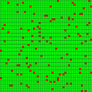
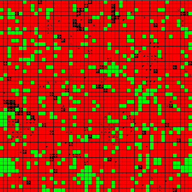
Figure 1. Example of an Initial State at t = 0 and t = 50 (Jump Mutations) - 4.23
- The landscapes created for this simulation were 50 x 50 cells, each of which could be populated by a single good cell (green) or infected cell (red). The landscape size was chosen to allow a large field of agents, so that resistance distributions would be well represented. A set of 100 "initial condition" snapshots was generated and stored for use under each experimental condition. Each snapshot was created by randomly placing a small set of initial infected cells with empty resistance repertoires, then running 50 update steps to allow for infection and pathogen mutation. Figure 1 displays an example of two snapshots, one at t=0 with few infections (left) and one at t=50 with infection growth and variations due to mutation (right). These initial steps represent the duration in which no treatments are applied, due to either diagnosis time or planning time for an intervention. The length of this initial period was intended to allow the model to approach the steady-state infected population for an untreated case. This burn-in period is also intended to form clusters of infected agents with similar resistances, representing a more realistic condition than random seeding alone.
Algorithm 1: Initial State Generation Algorithm
LET Random() generate a uniformly random number in [0,1]
LET Healthy() be a function that creates a healthy agent
LET Infected(Resistances) be a function that creates an infected agent, whose pathogens have certain set of resistances (Resistances)
LET Step(state, MI, T)be a function that generates a new landscape state, based on the current state (state), the mutation inheritance (MI), and the current treatment (T)
LET s0 be the vector of 100 landscape states
FOR state in s0:
## Randomly start with approximately 5% of infected cells
FOR cell in state:
IF Random() > 0.95:
cell = Infected(Resistances = {})
ELSE:
cell = Healthy()
## Update the landscape for 50 steps with no treatment
FOR t in [1, …, 50]:
state = Step(state, MI=0, T={}) - 4.24
- Memoryless mutation was employed to generate these initial states, as outlined in Algorithm 1. It should be noted that this method does not precisely reflect the "initial growth" of strains non-memoryless mutation (or other forms of memoryless mutation). However, the advantages of all conditions starting with the same initial states outweighed the impact of slightly more accurate initial states, since the focus of these experiments was the comparison of evolved resistances under selection pressure. For this reason, the variation and resistance drift used to generate the initial conditions was of diminished importance.
- 4.25
- The experiment consisted of eleven distinct intervention conditions, each repeated for the two distinct types of mutation (memoryless and random walk). Every combination of mutation and intervention was run for each of the 100 initial snapshots. A run consisted of a total of 500 steps, including the fifty occurring during the initial growth stage (so 450 steps during which an intervention was run). The computer cycles to simulate an individual run were dependent on the number of infected cells at each time step, making the run-time highly dependent on the nature of the intervention. Interventions that eliminated all infection proceeded much faster, as the remaining steps required minimal calculation.
Table 6: Treatment Notation Sets Bits Decimal Value {} 000 0 {0} 001 1 {1} 010 2 {2} 100 4 {0, 1} 011 3 {0, 2} 101 5 {1, 2} 110 6 {0, 1, 2} 111 7 - 4.26
- An intervention is defined as a course of treatments applied over time. Three treatment options are available in the model, which may be applied individually or simultaneously in any combination. Treatment combinations will be expressed in this context using set-wise notation, but it should be noted that the model internally represents these using bits in an unsigned integer. The total treatment combination is represented in the model as the decimal value for a three bit binary number, with each bit representing of a given treatment option is currently applied. Treatment options will be referred to by their bit position, so treatment # 0 is applied only when the zero bit is true (making the decimal value odd). For convenience, Table 6 displays the conversions for treatment notation. Let the variable T be defined as the treatment applied in the model.
Algorithm 2: Model Runs Under Interventions
LET s0 be the vector of 100 initial states
LET MI be the mutation inheritance setting for the run
LET Intervention(t)be a function that returns a treatment T as a function of the current time step (t)
LET Step(state, MI, T) be a function that generates a new landscape state, based on the current state (state), the mutation inheritance (MI), and the current treatment (T)
FOR state in s0:
FOR t in [51, 500]:
T = Intervention(t)
state = Step(state, MI, T)
- 4.27
- Each intervention was run for each of the 100 initial conditions, as described in Algorithm 2. Interventions are categorized into one of four basic types: control, single treatment, overkill, and cycling. A control intervention, with T = {} always, was run as a baseline. Single treatment interventions tested the impact of one treatment consistently applied over time. Two single treatment interventions were tested using different options to establish that no bias for a particular treatment or resistance existed. Overkill interventions consisted of any intervention where two options were applied simultaneously, for any span of time. Overkill was used to test the effect of applying either two or three treatment options simultaneously. Cycling interventions consisted of multiple treatment options alternating over the course of the run. In these models, the length of cycles was taken to be equal for each option. The set of interventions examined is contained in Table 7. For all interventions, the total time interval was between t = 50 and t = 500. In this table, the percent sign is used to represent the modulus operator.
Table 7: Intervention Types Intervention # Treatment (T) Over Time (t) Description 0 T = {} Baseline 1 T = {0} Single treatment 2 T = {1} Single treatment 3 T = {0,1} Double overkill 4 T = {0,1,2} Triple overkill 5 T = {0} when (t % 50) < 25
T = {} elseInconsistent single treatment 6 T = {0,1,2} when (t % 50) < 25
T = {} elseInconsistent overkill treatment 7 T = {0} when (t % 50) < 25
T = {1} elseCycling two options; 25 step intervals 8 T = {0} when (t % 100) < 50
T = {1} elseCycling two options; 50 step intervals 9 T = {0} when (t % 75) < 25
T = {1} when 25 <= (t % 75) < 50
T = {2} elseCycling three options; 25 step intervals 10 T = {0} when (t % 150) < 50
T = {1} when 50 <= (t % 150) < 100
T = {2} elseCycling three options; 50 step intervals 
Figure 2. Healthy Cell 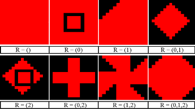
Figure 3. Infected Cell Variants - 4.28
- The PS-I landscape viewer was configured to display pathogen strains saliently, allowing for effective representation of the distribution of strains across the landscape to support the distribution data. In the PS-I landscape, a good cell is represented by a green square (Figure 2). Infected cells are represented by red squares containing various patterns which represent the set of pathogen resistances (Figure 3). Empty red squares have no resistances to treatment (R={}), while those at the bottom right are fully resistant to all three treatment options (untreatable, R={0,1,2}). The spread of untreatable resistance is a highly negative event, analogous to a staph infection that is fully resistant to antibiotics.
- 4.29
- Data was collected from 20 trials, where each trial was a unique combination of an intervention (from Table 7) and mutation inheritance (jump vs. walk). Each trial had 100 runs, where each run started from one of the initial conditions generated by Algorithm 1. For each intervention trial, the simulation script recorded a count of good cells and of each type of infected cell for each time step of each run. The code for the current treatment was also marked for each time step. This level of granularity captures the full time series of infection dynamics for the model and enables analysis of rates of resistance acquisition and aggregate infected cell populations.
- 4.30
- TCL scripts can be executed within the PS-I environment. These scripts were employed to implement Algorithm 1 generate initial state snapshots and Algorithm 2 to run the simulation under different intervention conditions. The scripts necessary to replicate this experiment are hosted with the model specification. Statistics were collected using PS-I's internal capabilities, supplemented by TCL logging.
Results: Evolution of Resistance
- 4.31
- Data analysis for this experiment focuses on the total number of infected cells on the landscape and their distribution of resistances. The focus of analysis is upon comparisons between different interventions, as the model parameters are not calibrated to match a particular real-life situation. Interventions are compared based upon their final state (t = 500) values and their rates of acquiring resistances. The length of the interventions was chosen so that the final state captures steady state values.
- 4.32
- The total set of runs for each trial was reduced to a median run and a representative run. These runs follow the same data format as a standard run, with the count of each pathogen strain listed for each time period. In the median run, the count of each type of infected cell is the median value of that strain's count for a given time step across all runs for that trial. The median run minimizes the variance of each strain for each time step. The representative run uses the full set of values from one particular run monitored for that intervention. The representative run was the run with the minimal mean variance from all other runs in the trial set. Variance between runs is calculated as the cumulative RMS difference for each strain at each time step.
Table 8: Final Infected Cell and Average Resistance Counts for Median Run (t = 500) Intervention Jump Mutations Walk Mutations # Treatments # Infected Cells Resistances Per Infected # Infected Cells Resistances Per Infected 0 Baseline: {} 2182 0.31 2182 0.49 1 Single: {0} 1361 1.09 1487 1.35 2 Single: {1} 1358 1.09 1489 1.35 3 Double: {0,1} 1339 1.92 1490 2.11 4 Triple: {0,1,2} 0 0 0 0 5 Inconsistent: {0} 2157 0.93 2170 1.35 6 Inconsistent: {0,1,2} 83 0.03 83 0 7 Cycling @25: {0},{1} 1338 1.89 1496 2.11 8 Cycling @50: {0},{1} 1354 1.87 1493 2.11 9 Cycling @25: {0},{1},{2} 0 0 913 2.98 10 Cycling @50: {0},{1},{2} 0 0 1434 2.96 - 4.33
- The model was run with a 50x50 landscape, allowing 2500 total positions. It should be noted that all positions not occupied by infected cells are occupied by good cells, so their count will not be listed, but is readily calculable. Table 8 lists the infected cell counts and resistances per infected cell at the end of the median run for each intervention. The values for the median run are close to the mean run, except for resistances when pathogens tend to be eradicated. The median values are useful in this case as they remove the noise generated by outliers, which are examined separately.
Median Run Analysis of Resistance and Infection Survival
- 4.34
- Table 8 displays the end-state of the median run for each condition, in terms of the number of infected cells present and the average number of resistances for each infected cell. The interventions were in general not very effective, due to the relatively high mutation rate of the infected population and its large initial size of over 2000 infected cells. This behavior was expected, given the parameters of the model. An infected cell population occupying more than a few dozen cells could be problematic. By these standards, only triple overkill was uniformly effective. The number of infected cells in steady state depends on model parameters, in particular the probability of a resistant cell being cleared by a treatment type that it resists. This value explains much of discrepancy between the baseline intervention when compared to the single treatment intervention (e.g., Intervention 0 vs. Intervention 1).
Emergent Natural Selection
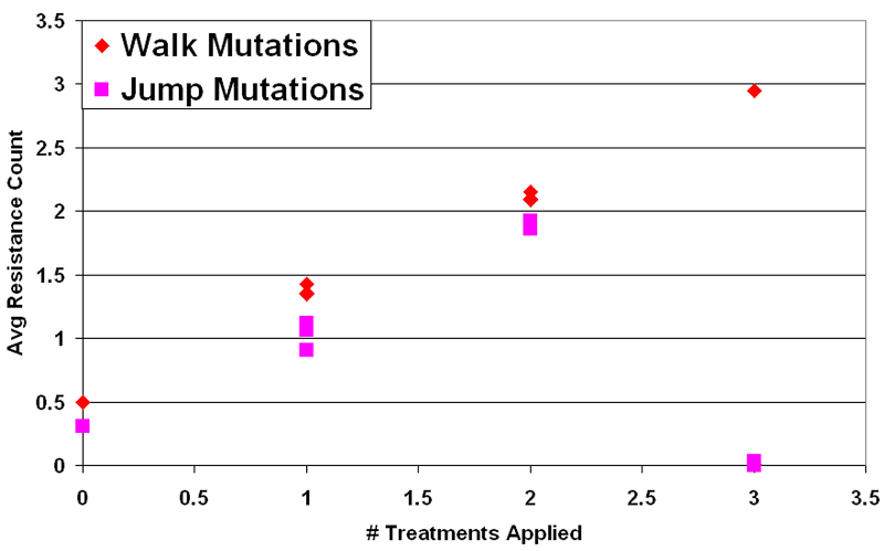
Figure 4. Mean Resistance (Median Run) vs. # Treatments in Intervention - 4.35
- The first important result is that natural selection occurs between pathogen types in this model. Any treatment option employed as a selection pressure against pathogens fosters an increased average resistance level in the population. For every trial where a selection pressure was applied, the average number of resistances in the infected population at steady state approximately matched the number of treatment options employed. This can be observed in Figure 4, where the average number of resistances per infection scales linearly (nearly one-to-one) with the number of types of treatment applied. This held for all interventions employed, except during runs where the infected cells fully recovered (N ≈ 0). This indicates that cycling does not prevent long term acquired resistance under any of these conditions. Given a selection pressure, this model's pathogens either adapt or are made extinct.
Table 9: Resistances Matching Treatments in Intervention at t = 500 (Median Run) Intervention Jump Mutations Walk Mutations # Treatments Exact Match Superset Not Resisted Exact Match Superset Not Resisted 0 Baseline: {} 0.71 0.29 - 0.59 0.41 - 1 Single: {0} 0.83 0.12 0.04 0.67 0.33 - 2 Single: {0} 0.83 0.13 0.04 0.68 0.32 0.00 3 Double: {0,1} 0.95 0.00 0.05 0.88 0.11 0.00 4 Triple: {0,1,2} - - - - - - 5 Inconsistent: {0} 0.66 0.11 0.23 0.67 0.32 0.01 6 Inconsistent: {0,1,2} 0.00 0.00 1.00 0.00 0.00 1.00 7 Cycling @25: {0},{1} 0.93 0.00 0.07 0.87 0.12 0.01 8 Cycling @50: {0},{1} 0.91 0.00 0.09 0.86 0.12 0.02 9 Cycling @25: {0},{1},{2} - - - 0.98 0.00 0.05 10 Cycling @50: {0},{1},{2} - - - 0.96 0.00 0.05 - 4.36
- As shown in Table 9, the resistances acquired matched the set of treatments applied. For a resistance to be considered an exact match, it must contain all treatments employed in the intervention. This means that a cycle of treatment 0 and treatment 1 (such as in Intervention 7) is matched exactly only by infected cells with {0,1} resistance. This means that the resistances held by infections matched the types of treatments applied, when treatments where applied. The intervention where the resistances did not match the treatments applied was the inconsistent triple overkill case. From examination of the run data, this appears to be the result of this intervention taking a long time to treat the infected cells. A longer time horizon would probably put this trial's results back in line with the general patterns of either total eradication or dominance of exact matches.
- 4.37
- Examining these trends, it can be observed that the number of resistances is a linear function of the number of treatment types applied during the intervention, provided that infected cells survive. Walk mutations tended to survive treatment more than jump mutations in general, partly due to slight differences in their drift tendencies. This difference can be measured using the baseline case, and amounts to walk mutation infected cells tending towards 0.49 resistances in the mean, a 0.18 advantage over jump mutation infected cells. Removing the points where the pathogens were wiped out, the slope for walk mutations was 0.81 and the slope for jump mutations was 0.8, effectively identical. Examining each intervention separately, simultaneous application versus cycling did not appear to have a significant impact on long term resistance acquisition when infected cells survived. This can be observed in Figure 5, where the average resistance per infection depends primarily on the intervention condition rather than the mutation style.
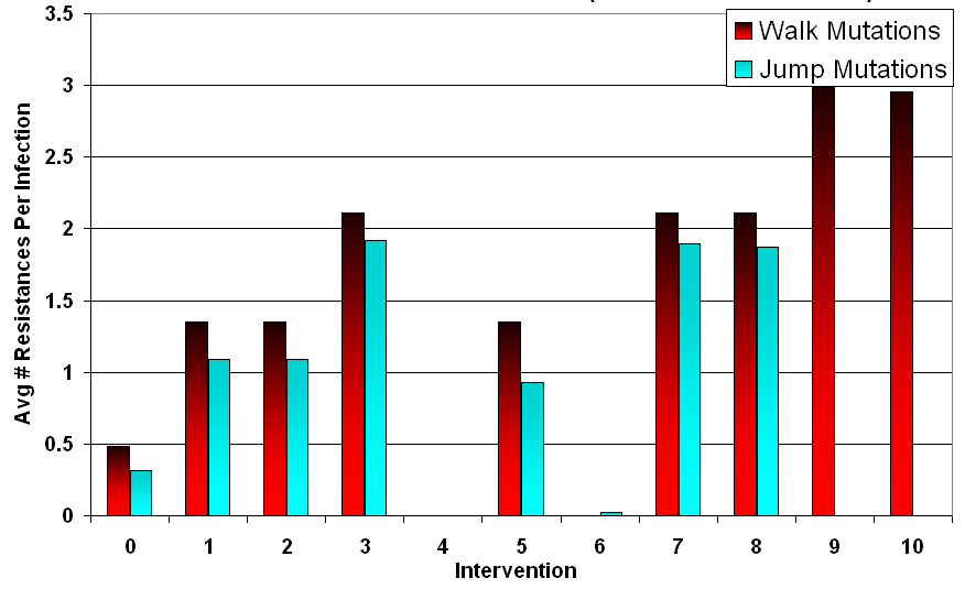
Figure 5. Average Number of Resistances at t = 500 (Median Run) Inconsistent Treatment Increases Infected Population (Including Resistant Ones)
- 4.38
- Literature states that inconsistent treatment increases the opportunities for population resistance, both for the median and in outliers. Studies of treatment to microbial pathogens have repeatedly shown this result (Wong et al. 1997;Lazarus & Sanders 2000). Breaks in treatment allow the infected population to regain numbers, giving more time for mutations to occur. After a treatment has been applied, the proportion of members resistant to that treatment will be higher with some probability. Allowing breaks in treatment increases the probability that resistance will be acquired and may increase the speed at which resistance is spread throughout the population. A slight reduction in average resistance was observed for jump mutations under intervention 5, treatment 0 applied inconsistently but this advantage was offset by a much greater average population throughout the run when compared to uninterrupted treatment (intervention 1). This meant that while the infected cells had lower average resistance, they had a greater total number of resistant members.
Cycling Ineffective Against Walk Mutations
- 4.39
- A second finding from Table 8 was that infected cells in the walk mutation condition survived treatment cycles more than those in the memoryless condition. This advantage was particularly noticeable during interventions 9 and 10, which were cycles of three different treatments. The jump mutation infected cells consistently recovered to good cells, while walk mutation infected pathogens tended to adapt and flourish instead. Since many settings involve perturbations that are not entirely memoryless, this finding indicates that care should be taken before choosing to cycle treatments.
- 4.40
- For the jump mutations, cycling does not appear useful for influencing the long term behavior on either type of mutation but performs similarly to an overkill condition with the same number of treatments. For the median case, this statement holds true. Cycling by changing treatments every 25 steps or 50 steps had no significant influence on the long term infected population or final resistance distribution. For walk mutations, cycling was noted above as being uniformly worse than a simultaneous application of treatments. For jump mutations, cycling is effective but works no better than overkill in the median. Since there may always be uncertainty as to the nature of mutation for a pathogen population, this would seem to indicate that overkill should be preferred.
Time Rates of Resistance and Infection Persistence
- 4.41
- To look more closely at the increases in resistance, the time rate of resistance acquisition was examined by finding the number of steps required for the infected population to achieve its steady state resistance value. This amount of time was dependent upon the number of treatments applied in an intervention and the sequencing of treatments. The slopes for resistance acquisition under these different conditions are calculated in Table 10. The slope of resistance acquisition was calculated from the initial value at t = 50 until the first point whose resistance was within 0.1 of the final (steady state) resistance. Entries marked with an asterisk indicate where resistance was lost due to all infected cells recovering. It should be noted that while inconsistent treatment slowed the development of resistance, it did so at the expense of maintaining a large infected population that was unlikely to be removed.
* All pathogens wiped outTable 10: Resistance Growth Slope for Representative Run (Avg. Resistance/Time Steps) # Treatments Jump Mutations Walk Mutations 0 Baseline: {} 0.0015 0.008 1 Single: {0} 0.024 0.009 2 Single: {1} 0.024 0.004 3 Double: {0,1} 0.021 0.022 4 Triple: {0,1,2} -0.001* 0.001* 5 Inconsistent: {0} 0.012 0.004 6 Inconsistent: {0,1,2} 0.001* -0.002* 7 Cycling @25: {0},{1} 0.020 0.016 8 Cycling @50: {0},{1} 0.016 0.018 9 Cycling @25: {0},{1},{2} -0.001* 0.012 10 Cycling @50: {0},{1},{2} -0.001* 0.017 - 4.42
- As shown in the table, cycling treatments seems to slow the acquisition of full resistance. Delays in acquiring resistance were observed when comparing the double overkill case versus the same treatment used in cycles for both styles of mutation. These delays are misleading, however. Figure 6 shows graphs of the median resistance over time for the double-overkill case (Intervention 3) compared to the 25 step cycling case with two treatments (Intervention 7) and the 50 step cycling case (Intervention 8). This graph is representative of the resistance curves for each type of intervention. In this graph, the resistance curve for Intervention 8 (50 step cycles) begins to plateau when resistance passes a value of 1 at t=80 but then resumes sharply at t=100 when the second type of treatment starts. This means that resistance acquisition is stalled only after full resistance to the current treatment has been completely acquired. While this delays the total acquisition of resistance, it does so at the expense of letting the infected population grow without an effective treatment being applied. In this way, the delay provided by cycling is little better than providing no treatment at all.
.png)
Figure 6. Median Resistance over Time for Step Cycling Treatments (Walk Mutations) - 4.43
- The overkill treatments had a small advantage in stalling resistance acquisition when compared with single treatment or cycling (which initially acts as a single treatment). Returning to Figure 6, double overkill causes an initial delay to the acquisition of resistance until about t=75. After this time, a rebound occurs and resistance acquisition occurs more rapidly, however. The triple overkill intervention (Intervention 4) works differently however: all pathogens are eradicated, preventing resistance. This data indicates that multiple simultaneous treatments have the best chance at working but if they fail, adaptation is accelerated.
- 4.44
- This raises the issue of outliers - what happens when overkill fails and whether cycling treatments reduces the probability of catastrophic failure (an untreatable fully resistant infected population). The importance of outliers in population resistance cannot be overstated. Many problems tend recur over time or in new settings. Through repeated runs, the probability of encountering an outlier increases vastly. Selecting interventions that avoid catastrophic outliers should be considered an important part of intervention strategies.
Outlier Analysis: Full Resistance Case
- 4.45
- For walk mutations, it has already been established that overkill is uniformly superior to cycling. As a result, the outlier analysis focuses on the outliers for jump mutations to determine if cycling has an advantage in that case also. Jump mutations always have a small probability of mutating to full resistance. In the tail cases for jump mutations, overkill results in a catastrophic failure where multiple resistances are acquired at the same time. In a majority of runs, these mutations are surrounded by enough competing infected cells to impede their spread and fizzle out. During overkill treatment, competing pathogens are removed and a fully resistant strain may spread throughout the landscape of good cells. This condition will be referred to as an overkill backlash case. The mechanics of this event follow the amplification model of population resistance (Pettersson et al 2004). A time lapse of a run where this event occurred is shown in Figure 7.

Figure 7. Fully Resistant Strain Backlash During Intervention 4 Run - 4.46
- The treatment works effectively up until approximately step 165, when a small cluster of fully resistant infected cells is left isolated due to the effectiveness of treatment on the surrounding treatment-sensitive infected cells. This small cluster infects nearby cells until infected cells cover the landscape. This event leads to a set of landscape states where it is improbable that the treatment will lead to recovery of the infected population. The difference in resistance paths displayed in Figure 8, which compares the median run of intervention 4 with the backlash case. At approximately t=100, the catastrophic failure case (red line) acquires total resistance and diverges from the median case (blue line) where all infections are wiped out.
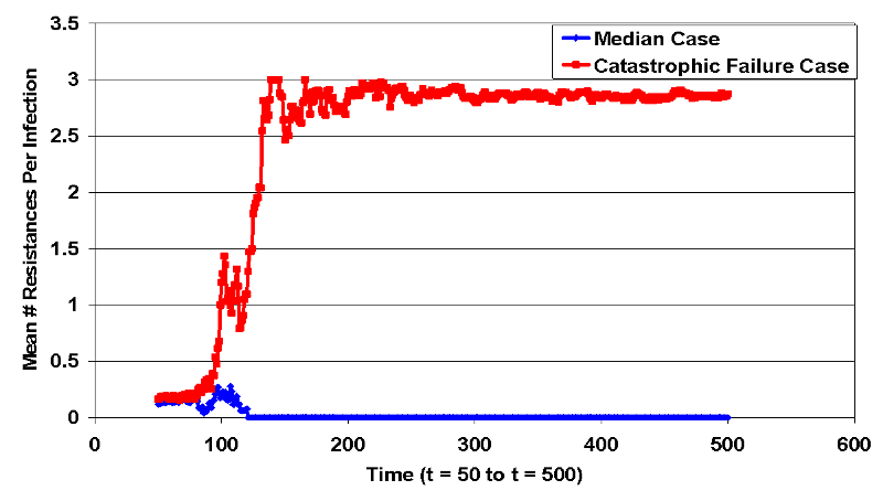
Figure 8. Bifurcation in Intervention 4 Resistances (Jump Condition) - 4.47
- The backlash event indicates a stochastic bifurcation (Song et al. 2010). Bifurcation in this context means that the Markov system contains classes of states that have limited communication (e.g., negative drift) or do not communicate. Certain initial conditions have a high probability to generate fully resistant pathogens rather than eradication. An example of this would be an initial condition where significant numbers of resistant infected cells exist at the start of treatment. Triple overkill treatment creates a bifurcation boundary that decreases the communication from states featuring fully resistant strains back to states with less resistant strains (since strains with no resistance are quickly eradicated). Cycling of multiple treatments does not maintain such a boundary, but creates a piecewise set of shifting boundaries over time. From this dynamic, it is possible that backlash outliers would not be observed during triple cycling for jump mutations.
- 4.48
- Table 11 lists the number of runs under each condition where fully-resistant strains existed at the end of the run. Based on this table, the overkill condition appears more likely to cause a fully resistant population of infected cells, since every time infected cells survived treatment 4 those infections were fully resistant. However, the cycling cases had only slightly fewer runs where fully resistant infected cells survived (10 for cycling vs. 13 for overkill out of 100 runs each). Since this difference was not statistically significant, an additional 300 supplementary runs were performed under treatment 4 (overkill) and treatment 10 (50 step treatment cycles).
Table 11: Overkill vs. Cycling on Fully Resistant Infection Survival (Jump Condition) # Treatment # Trials Where Any Infected Cells Remained # Trials Where Fully Resistant Remained 4 Triple: {0,1,2} 13 13 9 Cycling @25: {0},{1},{2} 18 10 10 Cycling @50: {0},{1},{2} 15 10 Table 12: Overkill vs. Cycling on Fully Resistant Infected Cells (Jump Cond., 400 runs) # Treatment # Trials Where Any Infected Cells Remained # Trials Where Fully Resistant Remained 4 Triple: {0,1,2} 32 32 10 Cycling @50: {0},{1},{2} 49 32 - 4.49
- Table 12 shows the results for 400 runs performed to determine if cycling reduced the incidents where fully resistant infected cells emerged. The results in Table 12 indicate that cycling was not more effective in preventing full resistance. While cycling was overall less effective and allowed less-resistant strains to survive in some cases, both treatment conditions allowed the same number runs where fully resistant infected cells survived. In both conditions, 8% of runs resulted in a fully resistant infected population. This indicates that overkill is more effective on both types of mutations. As such, this model indicates that treatment cycling should only be considered when there is a price for holding certain resistances.
Fitness Costs: Exploratory Case
- 4.50
- To examine if cycling could be more effective for the jump mutation case, this set of 400 initial states was run under different fitness cost conditions. Each initial state was run under each unique combination of values from Table 13. These parameter values were intended to replicate the interaction between the overkill intervention (4) and cycling intervention (10) under the jump mutation style, while varying the fitness costs of resistance. The resistance fitness multiplier (FR) was set between 0.05 to 1.00 in increments of 0.05. Each of these conditions was run once with per-resistance fitness enabled and once with per-resistance fitness disabled.
Table 13: Parameter Values for Fitness Cost Exploration Parameter Value Sets Description Resistance
Fitness Multiplier (FR)[0.05, 0.10, …, 1.0] Modifier on infection probability for resistant strains Per Resistance Fitness [0, 1] If 0, fitness multiplier applied once. Otherwise, compound the multiplier once per resistance.. Intervention (I) [4, 10] An intervention from Table 7, consisting of Treatments sequenced over time. - 4.51
- As in the immediately prior analysis, a count of the number of runs where fully-resistant cells remained at the end was counted for each condition. Clearly, imposing a fitness cost per resistance causes a greater total fitness cost on fully resistant strains. This causes a significant difference between the conditions, apparent in the fact that infections in the per-resistance fitness case were completely eradicated at a fitness multiplier of 0.8 rather than at 0.5 for the single-resistance case. To account for this, results were analyzed as a function of the overall fitness modifier for fully-resistant strains. For single cost resistance, the fitness cost for a fully resistant strain is equal to the fitness modifier (FR). For per-resistance fitness cost, the fitness modifier is compounded once for each of the three resistances held (FR3).
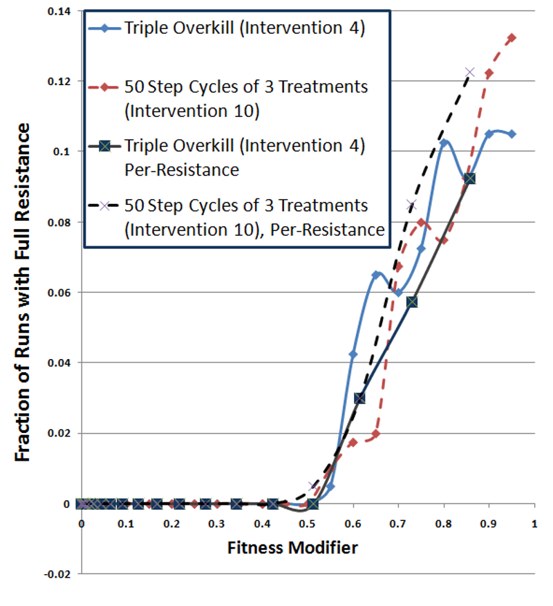
Figure 9. Fully-Resistant Survival Rate as a Function of Fully-Resistant Fitness Cost - 4.52
- Figure 9 plots the fraction of runs where a fully resistant strain survived as a function of the fitness cost for fully-resistant strains. Since these curves plot the fraction of runs where fully-resistant strains survived, larger numbers are worse. In this plot, the darker lines show per-resistance fitness cost conditions, while the lighter lines (red and blue) display single fitness cost conditions. The dashed lines represent cycling treatment and the solid lines show overkill treatment. The results for the two cycling treatments (dashed lines) track each other well, showing no major impact from per-resistance fitness. The overkill treatments also display results similar to each other. This indicates that fitness costs of fully resistant strains dominate the overall probability of a fully resistant strain surviving. This is somewhat expected, since resistance transitions are not incremental. Per-resistance fitness would have a larger impact on primarily inherited mutations (e.g., walk mutations).
- 4.53
- These results did not show an advantage for cycling, even when resistance carried fitness costs. While fitness costs hurt the overall survival rate of infections, cycling and overkill interventions performed comparably. In the single resistance cost cases (lighter lines), the only significant advantage for cycling (red dashed line) exists in Figure 9, at fitness costs of 0.6 and 0.65. However, the triple-overkill (solid blue line) alternately has the advantage elsewhere and the curves appear quite similar. The per-resistance cost curves (darker lines) show a possible advantage for overkill (solid black line) under per-resistance conditions (dashed black line), contrary to an advantage for cycling.
- 4.54
- The combined plot confirms that cycling does not demonstrate an overall advantage nor a pronounced disadvantage. Cycling and mixed strategies perform similarly, with the number of treatments being the dominant factor. Overall, this analysis finds little evidence for an advantage of cycling strategies over overkill strategies. Cycling may still have advantages where resistance carries a fitness cost under other conditions. Longer cycling periods or a mutation drift favoring loss of resistances may enable cycling strategies to outperform overkill strategies. With that said, these findings indicate overkill outperforms cycling under the conditions in this study and provides a more general and robust strategy against acquired resistance.
Conclusions and Future Directions
- 5.1
- An adaptive population will tend to overcome any finite set of treatments. This means that the effectiveness of any treatment is not just its ability to eradicate problems but also the number of uses over which it will be effective. This work extended the SIS model design to examine the relationship between anti-pathogen intervention strategies and pathogen acquired resistance to the treatments involved.
- 5.2
- A consistent finding across conditions was that the infection population would acquire the needed resistances unless they died out. A second finding was that varying the structure of the intervention (overkill, cycling, irregular) had an impact on the acquisition of resistance that was almost entirely controlled by the time of exposure to each treatment. This indicates that none of the tested methods extended the amount of effective use of a treatment within this model. The key exception to this was when the infection was eradicated, destroying the population "memory" of the selection pressure. At face this indicates that overkill has an advantage over other types of interventions.
- 5.3
- For a single trial, overkill is the most effective, having the highest likelihood of restoring all infected cells to good cells. Assuming many trials, outlier mutations are important for determining the most effective intervention. In this model and in many real life circumstances, the target population tends to adapt by a kind of greedy optimization. This greedy optimization by evolutionary processes should be containable through careful design of interventions. In such design the influence of outliers on acquired resistance cannot be understated.
- 5.4
- The probability of a resistant case spreading determines the expected number of times that a treatment can be used. Due to the relatively low probability of such a case, halving this probability could result in hundreds to millions of extra uses for a given treatment. For example, the triple treatment cycling for jump mutations was nearly as effective as the equivalent overkill at eradicating infected cells entirely. Even with a cost to resistance (e.g., a metabolic price à la Gillespie & McHugh 1997), triple cycling did not display an advantage in reducing the probability of an untreatable strain becoming dominant. However, further research exploring where cycling can outperform overkill treatments would be valuable, as only a limited number of conditions were explored in this study. Additionally, compensatory mutations that negate fitness costs for resistance were not explored in this study. The consequences of compensatory mutation are an area that warrants further study.
- 5.5
- Acquired resistance is an important dynamic of evolutionary systems, having significant repercussions on the ability to re-use the same treatments and strategies. This mechanism extends beyond traditional pathogens such as microbes and pestilence. Social harms also demonstrate acquired resistance in response to policy interventions, such as drug peddling, fraud, and terrorist cells (Murphy et al. 1990; Edelson 2003; Bell 2005; Jackson 2001). As such, acquired resistance is a significant issue in both the biological and social domains. While social issues were not focus of this examination, strategies to reduce pathogens without fostering resistance may also offer insights into their long-term management.
- 5.6
- The conclusions from this model transfer readily to a pure apprenticeship model with local duplication, which can be a useful analog for some social systems. Future work may model a resistance transmission mechanism based on communication and horizontal inheritance. This would allow the model to represent processes such as the communication of criminal practices among prison populations (Cuthbertson 2004). Such a mechanism would best be modeled on a specific context and should be considered an important piece of social models of resistance transmission. Horizontal transmission also has consequences for microbial pathogens, through mechanisms such as reassortment and recombination. Examining horizontal transmission implications and social parallels are possible future directions for this model.
- 5.7
- For many problems, completely wiping out pathogens without a chance of recurrence is a pipe dream. This makes managing adaptive resistance important: increasing the useful life of interventions makes it easier to manage recurring problems that are difficult or impossible to prevent entirely. Though the model explored is relatively simple, it captures fundamental dynamics of evolution and gives insight into the importance of outliers on the choice of interventions. This indicates a potentially fertile ground for exploration of methods to increase the expected lifespan of policies. Links between biological evolution and social adaptation afford the possibility of a common model for the study of acquired resistance. Hopefully these links will provide the basis for further research, in which agent based modeling can be a powerful tool.
References
-
ALONSO, A., Campanario, E. & Martinez, J.L. (1999). Emergence of multidrug-resistant mutants is increased under antibiotic selective pressure in Pseudomonas aeruginosa. Microbiology, 145(10), 2857-2862. [doi:10.1099/00221287-145-10-2857]
BELL, S. (2005). The martyr's oath: The apprenticeship of a homegrown terrorism. Missisauga, Ontario: Wiley.
BHATTER, P., Chatterjee, A., D'souza, D., Tolani, M. & Mistry, M. (2012). Estimating Fitness by Competition Assays between Drug Susceptible and Resistant Mycobacterium tuberculosis of Predominant Lineages in Mumbai, India. PLoS ONE 7(3): e33507. [doi:10.1371/journal.pone.0033507]
CRANDALL, K. (Ed.) (1999). The Evolution of HIV. Baltimore, MD: Johns Hopkins University Press.
CUTHBERTSON, I. (2004). Prisons and the education of terrorists. World Policy Journal, 27(3), 15-22.
DARWIN, C.R. (1859). On the origin of species by means of natural selection, or the preservation of favoured races in the struggle for life. London: John Murray.
EDELSON, E. (2003). The 419 scam: information warfare on the spam front and a proposal for local filtering. Computers & Security, 22(5), 392-401. [doi:10.1016/S0167-4048(03)00505-4]
GHEDIN, E., Sengamalay, N.A., Shumway, M., Zaborsky, J., Feldblyum, T., Subbu, V., … Salzberg, S.L. (2005) Large-scale sequencing of human influenza reveals the dynamic nature of viral genome evolution. Nature, 437(7062),1162-1166. [doi:10.1038/nature04239]
GILLESPIE, S.H., & McHugh, T.D. (1997). The biological cost of antimicrobial resistance. Trends in Microbiology, 5, 337-339. [doi:10.1016/S0966-842X(97)01101-3]
GUMBO, T., Louie, A., Deziel, M.R., Liu, W., Parsons, L.M., Salfinger, M. & Drusano, G.L. (2007). Concentration-Dependent Mycobacterium tuberculosis Killing and Prevention of Resistance by Rifampin. Antimicrobial Agents and Chemotherapy, 51(11), 3781-3788. [doi:10.1128/AAC.01533-06]
HÄGGSTRÖM, O. & Pemantle, R. (1998). First passage percolation and a model for competing spatial growth. Journal of Applied Probability, 35(3), 683-692. [doi:10.1239/jap/1032265216]
HANDEL, A., Longini, I.M. Jr. & Antia R. (2009) Antiviral resistance and the control of pandemic influenza: the roles of stochasticity, evolution and model details. Journal of Theoretical Biolology, 256(1), 117-125. [doi:10.1016/j.jtbi.2008.09.021]
JACKSON, B.J. (2001). Technology acquisition by terrorist groups: threat assessment informed by lessons from private sector technology adoption. Studies in Conflict & Terrorism, 24, 183-213. [doi:10.1080/10576100151130270]
JIANG, W., Sullivan, A.M., Su C. & Zhao, X. (2011). An agent-based model for the transmission dynamics of Toxoplasma gondii. Journal of Theoretical Biology, 293, 15-26. [doi:10.1016/j.jtbi.2011.10.006]
KERR, B., Neuhauser, C., Bohannan, B.J.M. & Dean, A.M. (2006). Local migration promotes competitive restraint in a host-pathogen 'tragedy of the commons'. Nature, 442, 75-78. [doi:10.1038/nature04864]
KLEVENS, R.M., Morrison, M.A., Nadle, J., Petit, S., Gershman, K., Ray, S., ... & Fridkin, S.K. (2007). Invasive methicillin-resistant Staphylococcus aureus infections in the United States. Journal of the American Medical Association, 298, 1763-1771. [doi:10.1001/jama.298.15.1763]
KOSHLAND, D.E. (2002). The seven pillars of life. Science, 295, 2215-2216. [doi:10.1126/science.1068489]
LAZARUS, A. & Sanders, J. (2000). Management of tuberculosis: Choosing an effective regiment and ensuring compliance. Postgraduate Medicine, 108(2), 71-84. [doi:10.3810/pgm.2000.08.1183]
LEVY, S.B., & Marshall, B. (2004). Antibacterial resistance worldwide: causes, challenges and responses. Nature Medicine, 10, S122-S129. [doi:10.1038/nm1145]
LÓPEZ-VILLAVICENCIO, M., Courjol, F., Gibson, A.K., Hood, M.E., Jonot, O., Shykoff, J.A. & Giraud T. (2011). Competition, cooperation among kin, and virulence in multiple infections. Evolution, 65(5),1357-1366. [doi:10.1111/j.1558-5646.2010.01207.x]
LUSTICK, I. (2002). PS-I: A user-friendly agent-based modeling platform for testing theories of political identity and political stability. Journal of Artificial Societies and Social Simulation, 5(3),7. Retrieved from https://www.jasss.org/5/3/7.html
MESSINGER, S.M. & Ostling, A. (2009). The consequences of spatial structure for the evolution of pathogen transmission rate and virulence. The American Naturalist, 174(4), 441-54. [doi:10.1086/605375]
MOUTOUH, L., Corbeil, J. & Richman, D.D. (1996). Recombination leads to the rapid emergence of HIV-1 dually resistant mutants under selective drug pressure. Proceedings of the National Academy of Sciences, 93, 6106-6111. [doi:10.1073/pnas.93.12.6106]
MURPHY, S., Waldorf, D. & Reinarman, C. (1993). Drifting into dealing: Becoming a cocaine seller. Qualitative Sociology, 13(4), 321-343. [doi:10.1007/BF00989408]
NACHEGA, J.B. & Chaisson, R.E. (2003). Tuberculosis Drug Resistance: A Global Threat Clinical Infectious Diseases, 36(Suppl. 1), S24-30. [doi:10.1086/344657]
ONAFUWA-NUGA, A. & Telesnitsky, A. (2009). The Remarkable Frequency of Human Immunodeficiency Virus Type 1 Genetic Recombination. Microbiology and Molecular Biology, 73(3), 451-480. [doi:10.1128/MMBR.00012-09]
PALUMBI, S.R. (2001). Humans as the world's greatest evolutionary force. Science, 293(5536), 1786-1790. [doi:10.1126/science.293.5536.1786]
PARSHANI, R., Carmi, S. & Havlin, S. (2010). Epidemic Threshold for the Susceptible-Infectious-Susceptible Model on Random Networks. Physical Review Letters 104(258701), 1-4. [doi:10.1103/physrevlett.104.258701]
PATTEN, B.C., Straskraba, M. & Jørgensen, S.E. (1997). Ecosystems emerging: 1. conservation. Ecological Modeling, 96, 221-284. [doi:10.1016/S0304-3800(96)00069-5]
PETTERSSON, M.E., Andersson, D.I., Roth, J.R. & Berg, O.G. (2005). The amplification model for adaptive mutation: Simulations and analysis. Genetics, 169, 1105-1115. [doi:10.1534/genetics.104.030338]
SONG C., Phenix, H., Abedi, V., Scott, M., Ingalls, B.P., Kaern, M. & Perkins, T.J. (2010). Estimating the stochastic bifurcation structure of cellular networks. PLoS Computational Biolology, 6(3), e1000699. [doi:10.1371/journal.pcbi.1000699]
WANG, J.Y., Lee, L.N., Lai, H.C., Hsu, H.L., Liaw, Y.S., Hsueh, P.R. & Yang, P.C. (2007). Prediction of the tuberculosis reinfection proportion from the local incidence. Journal of Infectious Diseases, 196(2), 281-288. [doi:10.1086/518898]
WANG, R.H., Jin, Z. & Liu, Q. X. (2011). The evolutionary dynamics of a spatial multi-strain host-pathogen system with cross-immunity. Nonlinear Analysis: Hybrid Systems 6, 741-753. [doi:10.1016/j.nahs.2011.05.008]
WANG, Y.C. & Lipsitch, M. (2006). Upgrading antibiotic use within a class: Tradeoff between resistance and treatment success. Proceedings of the National Academy of Sciences, 103(25), 9655-9660. [doi:10.1073/pnas.0600636103]
WONG, J.K., Gunthard, H.F., Havlir, D.V., Zhang, Z.Q., Haase, A.T., Ignacio, C.C., ... Richman, D.D. (1997). Reduction of HIV-1 in blood and lymph nodes following potent anti-retroviral therapy and the virologic correlates of treatment failure. Proceedings of the National Academy of Sciences, 94(23), 12574-12579. [doi:10.1073/pnas.94.23.12574]
ZUR WIESCH, P.A., Kouyos, R., Engelstädter, J., Regoes, R.R. & Bonhoeffer S. (2011). Population biological principles of drug-resistance evolution in infectious diseases. Lancet Infectious Diseases, 11(3), 236-247. [doi:10.1016/S1473-3099(10)70264-4]