
 Abstract
- Often new modeling and simulation software is developed from scratch with no or only little reuse. The benefits that can be gained from developing a modeling and simulation environment by using (and thus reusing components of) a general modeling and simulation framework refer to reliability and efficiency of the developed software, which eventually contributes to the quality of simulation experiments. Developing the tool Mic-Core which supports continuous-time micro modeling and simulation in demography based on the plug-in-based modeling and simulation framework JAMES II will illuminate some of these benefits of reuse. Thereby, we will focus on the development process itself and on the quality of simulation studies, e.g., by analyzing the impact of random number generators on the reliability of results and of event queues on efficiency. The "lessons learned" summary presents a couple of insights gained by using a general purpose framework for M&S as a base to create a specialized M&S software.
- Keywords:
- Continuous-Time Microsimulation, Framework, Plug-In, Demography, Modeling, Simulation
Introduction
- 1.1
- If modeling and simulation studies shall be executed, either a custom off the shelf product can be used or new software is developed to support these studies. If a new software product is needed either the new software product can be built from scratch or based on reuse.
- 1.2
- On a first glance the creation of a new software tool without too much reuse seems to be easier: one does not need to learn about the pre-built software packages to reuse, one does not need to trust the software developed by others, and considering the plethora of software products dedicated to modeling & simulation (M&S) reviewing these might get expensive. Finally, developing such a software product does not appear too difficult. However, recent literature about the quality of M&S software and studies performed warn against the dangers of this approach (Kurkowski et al. 2005; Merali 2010). Already in their technical report about SWARM, Minar et al. observe that "Unfortunately, computer modeling frequently turns good scientists into bad programmers. Most scientists are not trained as software engineers." (Minar et al. 1996, p.2). Software development involves many different tasks which need to be executed with care and which consume a considerable amount of time (Sommerville 2007). Thus developers, particularly those of smaller projects, may negate the need for (or even don't know of) proper software engineering until it is "too late" (Hannay et al. 2009). Also (Merali 2010) concludes that many problems in scientific computing can be traced back to the fact that scientists typically are neither educated nor trained as software engineers.
- 1.3
- When in the context of the project 'MicMac ( www.micmac-projections.org) - Bridging the micro-macro gap in population forecasting' a demographic microsimulation software, i.e., the Mic-Core, should be designed for being used by governmental institutions these considerations needed to be taken into account.
- 1.4
- The aim of the MicMac-project was "to develop a methodology and the associated software that offers a bridge between aggregate projections of cohorts (Mac) and projections of the life courses of individual cohort members (Mic)." (NIDI 2011). In demography aggregated projections of cohorts are the conventional way to conduct population projections. The standard methodology for this purpose are cohort component approaches (also denoted as macroprojections) (van Imhoff 1990), which commonly forecast population numbers according to age and sex categories. However, often these methods do not suffice when an adequate monitoring and forecasting of individual lifestyle and life courses is necessary to properly capture population development. Demographic microsimulation is a projection method that is suited for this objective. The idea of the MicMac project has been to run micro and macro projections in tandem, and to adjust microsimulation output relying on macroprojection output and vice versa. Our work has been focused on the Mic part of the project. Requirements for the Mic part had been: open source, easily portable, scalable, and supporting stochastic continuous-time micro models.
- 1.5
- In general, microsimulation tools are built from scratch and tailored for specific applications (such as a national tax or pension system). Exceptions are microsimulations implemented using the generic microsimulation language "ModGen" which is a shortcut for Model Generator (Statistics Canada 2011). ModGen can be used to establish microsimulation models that are variants of the Canadian microsimulation LIFEPATH (Gribble et al. 2003). However, it exhibits a few features which hampered its usage to implement the microsimulation tool of the MicMac project. It requires Visual Studio 2008 which is a commercial and complex software product, and therefore implies additional expenses. The source code of the ModGen library is not accessible. Furthermore, any new microsimulation application necessarily has to be a variant of LifePath, with all its pre-set assumptions and variables. As the MicMac microsimulation model has been conceptualized as a generic model (i.e., any kind of model parameters should be freely selectable), ModGen was not an option for the designers of the Mic-Core.
- 1.6
- Several agent-oriented modeling and simulation tools had been checked referring to their applicability building the MicMac microsimulation tool. However, the agent metaphor appeared not entirely fitting to the envisioned continuous-time micro models as the data available and the demographic simulation studies neither support nor require rich internal decision processes and sophisticated interactions between individuals. In addition, at the time of starting the project it was doubtful whether those would be sufficiently scalable to handle millions of individuals. In the meanwhile a lot of research efforts have been dedicated to address the problem of scalability in agent-oriented modeling and simulation tools, e.g., Repast (Collier & North 2011), though.
- 1.7
- For the MicMac microsimulation the conclusion was drawn to build a new software tool. Thereby, the development costs should be as low as possible - minding the fact that the potential developers are no software engineers and the research interests had not been the software as such but the insights to be gained by using the software.
- 1.8
- After a review of the state-of-the-art, JAMES II had been assessed to be appropriate for the implementation of the microsimulation tool. In contrast to libraries like SSJ a framework like JAMES II does not only provide specific functionality for reuse. It supports orchestrating the functionality to create specialized modeling and simulation tools (Himmelspach 2012).
- 1.9
- In the following we will describe experiences and results of using the M&S framework JAMES II for developing the specialized M&S tool Mic-Core. At first we motivate the development of a general framework for M&S, identify requirements and needed functionalities, and describe the plug-in based architecture of JAMES II. At second we introduce the concepts of demographic continuous-time microsimulation, which need to be implemented in a M&S tool. Thereafter, we describe the realization of this tool, i.e., Mic-Core, based on the general M&S framework JAMES II. Based on data from the Netherlands, we construct a case study. Therefore, several experiments have been conducted which illuminate reliability, scalability, and applicability of Mic-Core. Finally, we conclude with a number of lessons learned.
Background
- 2.1
- The decision to realize the microsimulation tool of the MicMac project using a M&S framework brought together researchers from two different fields: framework developers cooperated with demographers. The background section reflects these two perspectives. First, we discuss the needs for a framework for M&S and we describe our solution. Then, we detail the application side and describe the intended type of model and the usage scenario.
A framework for M&S
Software design considerations for M&S
- 2.2
- During the last decades, software development for M&S has led to a considerable number of software products. Some of these software solutions are dedicated to single modeling means (Moss et al. 1998; Klügl & Puppe 1998), others are dedicated to certain computing paradigms (Park & Fujimoto 2007), and a few more are open for alternatives (Clark et al. 2001; Lee 2003; Perumalla 2005). Thereby, independent from the concrete application domains, any software for M&S has to cope with a number of basic requirements and it has to provide a set of basic functionalities (Himmelspach 2009).
- 2.3
- Simulation studies include developing a model and executing experiments with the model. These basic tasks determine the functionality all M&S software has to offer. M&S software should provide means to support building models, e.g., by modeling editors, by composing models, or by import and export formats to model repositories.
- 2.4
- Simulation software needs to provide efficient and effective support for experimenting with these models. Experiments with a model might imply a single simulation run, multiple runs (required for stochastic models), and even multiple configurations. E.g., to search for a particular parameter configuration to fulfill a certain property, different parameter configurations have to be calculated, each of which, in the case of a stochastic model, might imply multiple replications. Single runs, multiple runs, and multiple configurations need to be analyzed. E.g., to determine whether one run has already reached steady state and thus can be stopped, to determine whether the number of replications is sufficient according to the determined confidence interval or further replications are needed, or to determine whether the found configuration sufficiently fulfills the goal function of the optimization. In most cases, the simple toy duck approach, i.e., "to wind it up and let it run", will not be sufficient, thus additional support is needed. Thus, simulation software needs to provide a suitable portfolio of diverse methods to be exploited or to allow an easy integration of new methods. In the best case they should offer both.
- 2.5
- Basic requirements that all M&S software share are ensuring repeatability of experiments and employing only thoroughly tested and highly efficient software (Himmelspach & Uhrmacher 2009).
- 2.6
- Similarly to experiments in physics and cell biology, experiments performed on a computer with a formal model should be repeatable or at least reproducible. Only this allows readers to value and interpret the achieved simulation results. This implies that experiments should be well documented. This is currently often not the case. Pawlikowski et al. (Pawlikowski et al. 2002) and Kurkowski et al. (Kurkowski et al. 2005) identified insufficient experiment documentation as the major problem of M&S studies they analyzed and one central reason for the credibility crises of M&S. Interestingly, most of the documentation Pawlikowski et al. (Pawlikowski et al. 2002) and Kurkowski et al. (Kurkowski et al. 2005) missed in the simulation studies could have been retrieved and stored automatically, e.g., the seeds for and the random number generators used.
- 2.7
- Efficiency is another requirement that might affect the quality of the simulation results achieved. E.g., in extensive experiments Galan and Izquierdo identified validity problems in a model published by Axelrod (Galan & Izquierdo 2005). At the time of Axelrod, the authors state this type of extensive experimentation would have not been possible, due to the lack of computing power. However, missing computing power is still a problem. Thus, lack of computing power or lack of efficiency might endanger the validity of simulation results as it prevents or at least discourages a thorough experimentation even nowadays. To respond to the need of thorough experimentation, software for M&S needs to be scalable (Himmelspach et al. 2010). Often one cannot predict the computational needs of a M&S study before the model is being created. Thus, the software should be sufficiently flexible to cope with the computational demands arising later on. A general domain independent approach to scalability is to involve parallel computations of models. These might be parallel computations of parameter configurations or just multiple replications in parallel. Another approach is the flexibility to replace data structures or algorithms on demand. For example, an event queue that uses only the main memory to store data can be replaced by one using the hard disc as buffer to enable the computation of models which exceed the size of the machine's main memory.
- 2.8
- When we interpret simulation results, we depend on the correct functioning of the software. However, how can we be sure that the behavior that we analyze is due to the model and its implied semantics rather than due to artifacts introduced by the used software? Software development for M&S needs to cover the steps of any software development (Ribault et al. 2009), including the definition of requirements, design decisions (architecture of the software), team formation, validation of the implementations, documentation and so on. These do not guarantee a good software product but they are steps towards improving the quality.
- 2.9
- Considering the time needed to come up with a reliable software product for M&S that offers all the needed functionalities, the question arises whether there is not a solution that saves development time and at the same time helps circumventing some of the aforementioned problems. One answer is software reuse, see, e.g., the discussion on software in science (Hannay et al. 2009; Merali 2010) and for M&S software (Ribault et al. 2009). Minar et al. (Minar et al. 1996) wrote 1996 in their technical report about SWARM: "Once a field begins to mature, collaborations between scientists and engineers lead to the development of standardized, reliable equipment (e.g., commercially produced microscopes or centrifuges), thereby allowing scientists to focus on research rather than on tool building. The use of standardized scientific apparatus is not only a convenience: it allows one to "divide through" by the common equipment, thereby aiding the production of repeatable, comparable research results." Thus, according to Minar et al. reuse is a reliable way to allow the effective production of credible M&S results.
- 2.10
- Motivated by these considerations we built a general framework for M&S, based on a flexible architecture which supports both, reuse and expendability.
Plug'n simulate - A framework for M&S: JAMES II
- 2.11
- Numerous software architectures can be used to realize M&S software (Ribault et al. 2009). We decided to realize a modeling and simulation framework (JAMES II) based on a plug-in based architecture, shortly named "plug'n simulate" (Himmelspach & Uhrmacher 2007b).
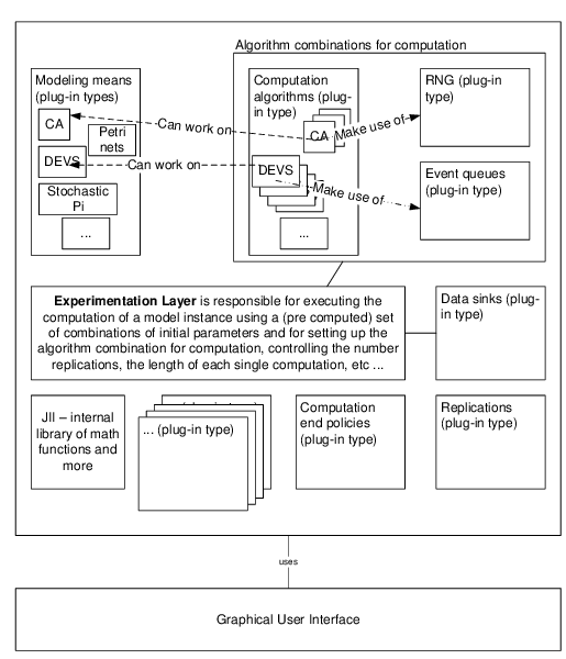
Figure 1. Overview of some of the JAMES II (JII) plug-in types and their internal interplay. The figure additionally sketches the experimentation layer of JAMES II which controls the execution of experiments making use of all the plug-ins. - 2.12
- The architecture allows to integrate any technique for M&S into the framework (and into any software built based on the framework) via so called plug-in types (extension points) which provide well defined interfaces and the means to automatically select an alternative from the list of alternatives installed for each of the techniques. Internally JAMES II integrates these extensions in control flows. Extending JAMES II by yet not supported functionality means to integrate a new plug-in type that allows including the functionality as a plug-in. Likewise, providing an alternative for any of the techniques supported can be done by adding a plug-in (Himmelspach & Uhrmacher 2007b). Any such extension can be used by any software built on using JAMES II.
- 2.13
- In Figure 1 some of the plug-in types created for JAMES II as well as their interplay are sketched. Another important part of the implementation, the experimentation layer (Himmelspach et al. 2008) allows full control over experiment types (e.g., parameter scans, optimization), and associated therewith over parameters (e.g., computation end policies, number of replications) (Ewald et al. 2010). This experimentation layer combines the diverse plug-in types (techniques) involved in simulations and can be reused for any application out of the box. At the end of 2011 already more than 600 extensions for about 80 extension points have been created. Thereby JAMES II does not enforce any reuse of its parts. Any user of the framework is free to choose which functionality he/she wants to apply.
- 2.14
- The core JAMES II framework does only depend on the Java JRE. This makes it easier to reuse the code as no further dependency needs to be taken into account.
- 2.15
- Further on its plug'n simulate architecture lends itself to experiments with algorithms. Usually algorithms under test are added as a plug-in to the system. Thus, during testing the algorithms, all alternative algorithms can be plugged in and evaluated in the same environment, e.g., (Himmelspach & Uhrmacher 2007a; Ewald et al. 2009). Thereby, trust in the correct functioning of newly developed plug-ins and insights into their performance can be gained. As the performance of algorithms depend largely on the model, to have alternative algorithms/data structures which can be used for the same tasks is mandatory for achieving "optimal" performance if the models to be computed vary (see paragraphs 4.14 - 4.19). This helps on the scalability issue and it helps to create efficient specialized M&S software based on JAMES II.
- 2.16
- JAMES II is already being used in various application areas. Specific modeling means have been developed for the different application areas and are provided as plug-ins in JAMES II. E.g., for the applications in the area of systems biology, variants of the stochastic pi formalism have been developed, e.g., (John et al. 2010), as well as rule-based languages, e.g., (Maus et al. 2011). Variable structure variants of the DEVS formalisms have been developed which are currently used for testing software in virtual environments (Steiniger et al. 2012). In all these approaches, a similar avenue has been followed: at first we identified what shall be expressed (the intended semantics), then we looked into how to express it (the syntax) and based on this, support for modeling and for computing the models have been realized in JAMES II (if no suitable modeling approaches and computation algorithms already exist in JAMES II).
- 2.17
- JAMES II can be downloaded at http://www.jamesii.org and is distributed under the JAMESLIC license which allows free reuse for commercial and non-commercial projects.
Application: demographic microsimulation
- 2.18
- The basic idea of a microsimulation is to model and simulate the behavior of micro units in order to get insights about the dynamics of a system, like a population or an economy (Orcutt 1957; Orcutt et al. 1961). In a demographic microsimulation the central micro unit is the individual life course, which is characterized by a sequence of demographic events, e.g., birth, marriage, death, and the time spans between these events. It offers the functionality to study individual behavior, inter-cohort variation, interaction among individuals, and interaction between individuals and macro units along calendar time and/or age. Despite a considerable regularity of demographic behavior, the order and age- and period-specific incidence of demographic events varies between individuals. Therefore, individual life courses are appropriately modeled by stochastic processes (Bartholomew 1973; Mayer & Tuma 1990).
- 2.19
- In microsimulations time can be treated differently, either as being discrete (usually in units of years or months) or as being continuous. In discrete-time microsimulations, time advances in discrete steps, i.e., the time axis is discretized. At each step individual attributes and behavior are updated. In contrast, a continuous-time microsimulation features a continuous time scale, along which events occur, i.e., an event can occur at any instant in time. Pros and cons of both approaches are discussed in (Galler 1997) and (Zinn et al. 2009). For the MicMac project the continuous-time approach was considered to be the appropriate choice.
- 2.20
- Each demographic microsimulation comprises a virtual population and a stochastic model of individual behavior (Willekens 2009). The virtual population consists of individuals that are distributed over the attribute categories of the model (sex, marital status, educational attainment, for example) and across ages (commonly given in single years of age). This model population evolves over time, individuals experience demographic events based on the stochastic model over their lifetimes. A standard approach to describe in a continuous-time microsimulation setting individual behavior is using a continuous-time multi-state model (Bartholomew 1973; Andersen & Keiding 2002; Gampe & Zinn 2007). The model state space ψ is a set of states that the individuals of the virtual population can occupy.
- 2.21
- The state space is determined by the problem to be studied and contains the relevant demographic states that need to be considered. An obligatory part of the state space is "dead", a risk to which each individual is always exposed to. Any demographic event, like getting divorced or childbirth, changes an individual's state.
- 2.22
- Three different options exist for an individual to enter the model population: (1) being member of the initial population, (2) birth, or (3) immigration. An initial population contains the distribution of population members according to the states that they occupy at simulation starting time. Individuals leave the population either by death or by emigration.
- 2.23
- In a continuous-time multi-state model, each individual life course is formulated as a trajectory of a non-homogeneous continuous-time Markov Chain (NHCTMC) Z(t), t ≥ 0, where t maps the time span over which we "observe" an individual life-course. The time t is set to zero when an individual enters the virtual population. As long as the individual is part of the virtual population, t evolves along the individual life time.
- 2.24
- Each NHCTMC is fully defined by the two-dimension process (Jn,Tn)n∈N0. Here (Jn)n∈N0 is a Markov Chain that maps all states that an individual occupies and (Tn)n∈N0 reports the sequence of the corresponding transition times. The waiting time that an individual remains in a state Jn is then determined by Wn = Tn+1 - Tn.
- 2.25
- Distinct from the process time Tn are calendar time and age. Depending on the application at hand, process time (indicated by the transition times of the process) can be mapped into age and calendar time: The function A(Tn) maps the age at Tn and the function C(Tn) the calendar time at Tn.
- 2.26
- The propensity of an individual to change his/her current state si at model time Tn, age a and calendar time x is given by the transition rate (or hazard rate) λsi,sj(x,a), si,sj ∈ ψ, x,a ∈ R0+, associated with process Z(t):

(1) - 2.27
- If the transition rates of the process are known, the distribution functions of the waiting times can be derived. Assumed an individual enters at calendar time x and age a a state si that is not the death or the emigration state then the individual will eventually experience a further transition in the future. Then the waiting time in state si until moving to another state sj can be simulated using the inversion theorem (Rubinstein & Kroese 2008). We denote a variate of a standard uniform distribution by u. A random waiting time wsi,sj from the correct distribution can be obtained by
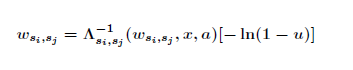
(2) where si,sj ∈ ψ, si≠sj and
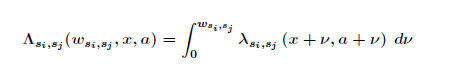
(3) is the so called integrated hazard. According to a competing risk setting (Wolf 1986; Galler 1997), we compute for all possible destination states waiting times and pick the shortest one wsi,sj* to state j*. Consequently the individual under consideration experiences his/ her next state transition to j* at age a + wsi,sj* and calendar time x + wsi,sj*. This computation of the "shortest" waiting times is repeated for each individual of the model population until the simulation stop time has been reached or all individuals have left the population (due to death or emigration).
- 2.28
- In order to forecast population numbers using the presented approach, the user has to provide an initial population and transition rates for all feasible transitions that individuals may experience during their lives. Commonly, for their estimation statistical methods of event history analysis are applied to retrospective or prospective life histories reconstructed from longitudinal data and/or vital statistics. Assumptions about future rates/probabilities then define the projection scenarios. More details of how to employ a continuous-time multi-state model in order to describe a microsimulation are given in (Gampe & Zinn 2007; Zinn et al. 2009).
Realization of the microsimulation based on JAMES II
-
Implementation
- 3.1
- Whenever JAMES II shall be used as a base for new M&S software a number of decisions have to be made in the beginning:
- Can any of the existing modeling means be reused or does a new one has to be integrated?
- Is a specialized user interface needed?
- 3.2
- If none of the existing modeling means suffices, at least an "executable model" and a "computation algorithm" have to be provided as plug-ins installed for the corresponding plug-in extension points. In JAMES II "executable models" are efficient classes that hold a parameterized instance of a model to be computed. The "computation algorithm" is the algorithm which computes the model. For the Mic-Core, we had to integrate these two parts because JAMES II did not provide support for modeling means that capture the intended semantics as described in paragraphs 2.18 - 2.28 so far. In addition, the decision was made to build a new, specialized and thus simpler user interface than the one that JAMES II provides. The experiment environment, data sinks, data storages, and basic M&S functionality are already available in JAMES II and ready for reuse.
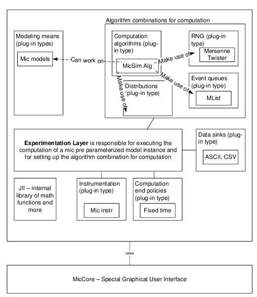
Figure 2. Overview of some JAMES II functionality that the Mic-Core software applies. - 3.3
- As a result, the Mic-Core consists of two plug-ins: an executable modeling plug-in (see Figure 2, "modeling means"), and a computation algorithm plug-in (see Figure 2, "algorithm combinations for computation").
- 3.4
- A model based on the Mic-Core modeling plug-in consists of two entity types: the population which comprises a set of individuals. Both are represented as interface and as class((I)Population, (I)Individual). This allows employing alternative implementations of the interfaces at later stages, e.g., if models cannot be completely held in the memory of the computer used or if alternative implementations promise a speed-up.
The algorithm to compute the model is based on the classical "hold" loop. In an event queue all scheduled events for the individuals are hold (at most one event per individual). The template for simulation algorithms in JAMES II requires implementing this functionality in the nextStep method (see Algorithm 1). This method computes the next state of the model - thereby the step can be the next integration point, the next step in discrete stepwise model, or the next event to compute in a discrete event based model. Everything else, i.e., run control (start, stop, pause), looping (including computation end condition evaluation), a.s.o. is automatically handled by corresponding "computation algorithm" classes in JAMES II.
public void nextStep() {
  Event event = eventQueue.dequeue();
  List newEvents = computeTransition (event);
  for each newEvent in newEvents do
    eventQueue.enqueue (newEvent);
  }
}
Algorithm 1. A step from the main loop of the computation algorithm comprises event fetching, execution of the transition, scheduling of new events. This refers to the classical "hold" operation in discrete event based computations. - 3.5
- In each step we have to dequeue the event with the minimal time stamp, compute the next state transition of the related individual, and enqueue the new events. The computeTransition method determines the new events to be scheduled based on the continuous-time multi-state model described in paragraph 2.18 - 2.28. During simulation individuals might be added or be removed from the population (due to birth, death, or migration). Hence, if individuals are added more than one new event might be returned, or none, if an individual is removed. A simulation run is completed when either all individuals are removed from the model population (the event queue is empty) or a pre-set simulation stopping time or condition has been reached. Subsequently, after a completed computation, for further analysis the simulation output can be stored using an adequate data sink plug-in that is provided by JAMES II.
- 3.6
- Instrumenters are responsible for selecting the data to be observed and to be recorded. Thus, not all data are necessarily stored. Data recording is done with the CSV-file based data recording mechanism provided by JAMES II.
- 3.7
- A more detailed description of the implementation of the Mic-Core and its workflow is given in Zinn et al. (2009). The Mic-Core and related material such as a manual and data examples can be downloaded at http://www.demogr.mpg.de/cgi-bin/micmac/login.plx. It is available as free software but comes with a license that fixes its usage for non-commercial purposes only.
Model specification
- 3.8
- Before performing an actual simulation run, the microsimulation model has to be specified. For this purpose, the Mic-Core requests
- the age range, over which the population shall be considered, and for which age-specific transition rates have to be provided,
- the period over which the simulation should be run, i.e., the starting year and the end-year for the simulation run,
- the age- and time-specific transition rates for all possible transitions in the model,
- the initial population, that is, the number of individuals in the different states of the model, classified by age, at the starting point of the simulation, and finally,
- the sex ratio (proportion of females to total number) that shall be applied to determine the sex of a newborn.
- 3.9
- The age- and time-specific transition rates and the initial population have to be provided via two input files. The consideration of immigration flows demands two further input files: one file comprising the numbers of immigrants given according to immigration date, age at immigration, and attributes of immigrants. The other file contains transition rates describing the behavior of immigrants once they have entered the population. A comprehensive description of the structure and the content of these files can be found in Zinn & Gampe (2011). Here, also detailed information on the kind of the input data required by the Mic-Core is given. Using R we have implemented procedures that allow deriving the empirical input data for the simulation and to construct the input files. (R is an up-to-date software environment for statistical computing. It is free and open-source and can be downloaded at http://cran.r-project.org/.) These procedures have been set up in the so called pre-processor of the Mic-Core (Gampe et al. 2010). (The pre-processor and a corresponding manual can freely be downloaded at http://www.demogr.mpg.de/cgi-bin/micmac/login.plx.) By means of a simple GUI the Mic-Core asks for the age range, the simulation time horizon, the sex ratio, and where to find the required input files.
- 3.10
- An instance of the model reading mechanism of JAMES II is used to read the input data, and to instantiate the model. Thus, the model to be experimented with can be exchanged without the need to modify in the Mic-Core any line of code.
Experiment setup
- 3.11
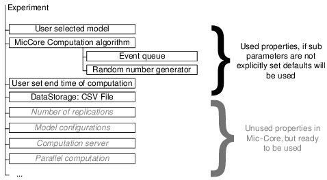
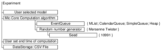
- JAMES II provides an experimentation layer which allows to setup and to control experiments (Himmelspach et al. 2008). Figure 3 shows a number of parameters of experiments in JAMES II as well as a small example to see what needs to be done to alter any of the parameters. For example, the Mic-Core uses parameters to specify a stop criterion, a data base to read input data from, a data storage for storing simulation output, an event queue, and a random number generator. All parameters set in JAMES II (pre-defined or computed on the fly) are handed over to a sequential or parallel computation task executor. Such proceeding facilitates the reuse of an experiment definition on single core machines as well as on machines containing more cores or even on distributed setups. The length of a simulation run can be determined by specifying either a simulation stopping time or conditions e.g., reaching the steady state.
- 3.12
- The number of replications can be defined in advance or it can be made dependent on certain characteristics of the simulation results achieved so far, e.g., by using a confidence interval. JAMES II's experimentation layer allows setting for each model parameter combination a different number of replications.
- 3.13
- Experimenting with the Mic-Core requires a rather simplistic experiment setup: it suffices to specify only a single parameter set, namely transition rates and an initial population. Running a microsimulation does not change any parameters of this set. Hence, replicating microsimulation runs with identical parameter settings only renders the derivation of the Monte Carlo variation in the microsimulation results. Changing, however, between microsimulation runs sub and input parameters allows to profit from the functionality of JAMES II's experimentation layer, and to evaluate different simulation setups. Generally, a microsimulation run stops if a pre-defined simulation end date has been reached.
Example of how to set a parameter of the experiment:

  // Data Storage
  exp.setDataStorageFactory(new FileDataStorageAttributeFactory());
  exp.setDataStorageParameters((new
ParameterBlock()).addSubBl(FileDataStorageAttributeFactory.PARAM_PATH, "./results"));
Figure 3. Setting experiment parameters. The figure shows a number of control parameters of experiments in JAMES II. Currently the Mic-Core computation algorithm uses two sub parameters: one to set an event queue and one to define a random number generator. The parameters in italics are currently unused but are ready for Mic-Core extensions. In addition, a code snippet (Java) is given showing what needs to be done to alter the experiment definition: Here we select a file based data storage for storing the simulation output.
Experiments
- 4.1
- To illustrate the capabilities of the Mic-Core and to highlight some of the benefits of using a framework regarding validation and efficiency, we describe in this section three different experiments. The first experiment explores whether the random number generator used introduces a bias into the results, and the second experiment deals with performance issues on computing the model, and the third experiment is about a demographic microsimulation using the Mic-Core. The first and second experiments are seen as examples for an additional potential of using a framework as a base for new software instead of a completely self-made software tool: alternatives being available and easily usable.
Demographic microsimulation: data and scenario
- 4.2
- To test different implementations in the Mic-Core we use data of a synthetic population that resembles the Dutch population. Here synthetic population means a population that evolves from a starting population built from different data sources, but still mimics reported attributes of the real Dutch population. In our experiments, starting at January 1, 2008, life courses of five cohorts are generated: individuals born in 1960, 1970, 1980, 1990, and 2000. The related total population numbers have been taken from EuroStat (EuroStat 2012):
born in 2000 born in 1990 born in 1980 born in 1970 born in 1960 total females 100946 99892 100843 129992 123748 555421 males 105151 105077 101407 131719 125923 569277 total 206097 204969 202250 261711 249671 1124698 - 4.3
- We simulate synthetic cohorts that correspond to one, two, ten, twenty, fifty, and one hundred percent of the number of actual individuals. The simulation starting time is January, 1, 2008, and the simulation stops at December 31, 2050. Individuals who belong to the cohort born in 1960 are 47 years and individuals born in 2000 are 7 years old at simulation starting time. In this example we focus on fertility behavior and changes in the marital status/living arrangement. As at older ages the marital and fertility history is usually completed, we consider life courses only until age 63. The state space of the considered model comprises the following individual attributes:
State variable Possible values sex female, sex educational attainment only primary school, lower secondary school, upper secondary or tertiary education marital status & living arrangement single, cohabiting, married fertility status up to four children mortality alive, dead 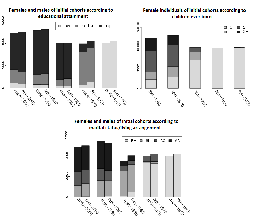
Figure 4. We consider five cohorts: individuals born in 1960, 1970, 1980, 1990, and 2000. The graphs depict the distribution of the five initial cohorts at simulation starting time. The graph on the top left shows the cohorts according to educational attainment; coding: low (only primary school), medium (lower secondary school), high (upper secondary or tertiary education). The top right graph shows the females of the initial cohorts according to children ever born. Cohort numbers according to marital status/living arrangement are given in the lower graph; coding: PH (living at parental home), SI (living alone), CO (cohabiting), MA (being married). - 4.4
- For each initial cohort, we have estimated population numbers cross-classified by sex, educational attainment, marital status/living arrangement, and fertility status using the method of iterative proportional fitting. The marginal distributions required for this purpose have been taken from the Family and Fertility Survey of the Netherlands (FFS_NL) and from EuroStat (EuroStat 2012). Figure 4 shows the respective distribution. During simulation women can become mothers. Both men and women might increase their educational level, or experience changes in their marital status. Individuals can leave the parental home, marry, cohabitate, become single, etc. The assumed transition pattern concerning changes in the marital status/living arrangement is given in Figure 5.
- 4.5
- All individuals are always exposed to death. For estimating fertility rates and transition rates of changing the marital status/the living arrangement, we have applied MAPLES. This method estimates age profiles from longitudinal survey data and had been developed during the MicMac project (Impicciatore & Billari 2011). The FFS_NL has served as data basis. Estimated fertility rates and rates of changing the marital status/living arrangement vary with age, but are hold constant over calendar time, using the year 2003 as reference year. Mortality rates have been taken from EuroStat2008 projections for the Netherlands (baseline scenario). They vary with age and calendar time. To quantify an individual's propensity of changing his/her educational attainment, we have used data provided in (KC et al. 2010). For readability, all applied transition rates are given in the appendix. Generally the Mic-Core allows the consideration of migration, however, for reasons of simplicity we only concentrate on persons who were born in the Netherlands.
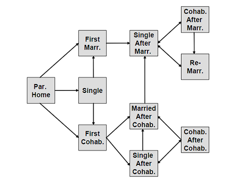
Figure 5. Transition pattern concerning changes in the marital status. Conducting experiments with a stochastic model
- 4.6
- The repeatability of simulation results on different machines and with different implementations has been recognized as sine qua non for the reliability of simulation models (Edmonds & Hales 2003). If the model to be computed or the computation algorithm contains stochastics one has to take special care of the pseudo random number generator (PRNG). Starting from a pre-specified seed, a PRNG produces always the same sequence of pseudo random numbers. The period is the maximum length of that sequence before the PRNG begins to repeat numbers. Therefore, the period length p of a PRNG is crucial for its applicability. Many different PRNG have been invented so far and often they have been considered to be faulty after a while, e.g., because of unwanted correlation patterns between random number variates. For example, the linear congruental generators (LCG) cause serial correlation between successive random number variates, and it is recommended to no longer use those (Press et al. 2007). Despite of their deficiencies, these days LCG are still rather popular because they are very efficient in terms of speed, easy to implement, and, correspondingly, portable code, parameters, and test toolkits are available. Many versions and enhancements have been done to counter the unwanted features of LCGs: The order of recursion has been increased from order one to a higher order, the length of periods has been enlarged, different types of PRNG have been combined, etc.
- 4.7
- To generally avoid any regularities in the pattern of the employed pseudo-random numbers, (L'Ecuyer & Hellekalek 1998) suggest drawing less than √p pseudo-random numbers. That is, if an application requires drawing many more random numbers than the square root of the period of the used PRNG is long, simulation results might be distorted. Commonly, however, no general statement can be made about the quality of a PRNG, as its suitability depends on structure of a particular problem. Minding this fact, we have checked whether different PRNGs have any influence on the results computed in the described use case. We have tested the following three PRNGs:
- RANDU which is an outdated LCG with a period of 231 ( √p ≈ 46341),
- Java random number generator which is a LCG with a period of approximately 248 (√p ≈ 16777216),
- Mersenne Twister which is based on a matrix linear recurrence over a finite binary field, and in its commonly used variant, MT19937, it has a period of 219937 - 1 (29968 < √p < 29969).
- 4.8
- To facilitate comparability each PRNG has been initialized with the same (arbitrarily chosen) seed. Considering our example, the average number of random numbers that have to be drawn can be computed as the product of the average number of individuals n that are considered during simulation, the average number of events e that they will experience over their life-course, and the average number c of competing risks per state transition. For different values of n, e and c, the table below gives an estimation of the amount of random numbers needed:
Size of initial population c = 3, e = 3 c = 3, e = 5 100% : n0 = 1124698 10122282 16870470 10% : n0 = 112470 1012230 1687050 1% : n0 = 11247 101223 168705 - 4.9
- In the table the size of the initial population n0 has been chosen as a lower bound of the average population size, i.e., individuals that enter the population during simulation are not counted in.
- 4.10
- All the numbers in the table are remarkably higher than the square root of the period of RANDU. On the contrary, the square roots of the periods of the java random number generator and of the Mersenne Twister exceed in almost all cases the required amount of random number variates. We are aware of the fact that taking n0 = 1124698 and c = 3, e = 5 yields an amount of needed random variates that is close to the square root of the period of the java random number generator. Notwithstanding, for our example, we expect overall no significant differences between the results that are obtained using the java random and the Mersenne Twister generator. The situation differs in case of RANDU: here a tuple of three in series drawn random number variates is always highly correlated (Marsaglia 1968; Hellekalek 1998), and this defect might bias the simulation results.
- 4.11
- All the listed generators are available as plug-ins in JAMES II; thus corresponding experiments can easily be done. The random number generator to be used is simply handed over to the computation from the experimentation layer.
- 4.12
- We run the Netherlands example using ten percent of the total size of the five cohorts and three different random number generators. Each experiment has been executed three times. As seeds we have (arbitrarily) chosen 213423, 5689, and 628164. That is, in total we have conducted nine simulation runs: one run per seed and studied PRNG. The average of random number variates produced per run was 1817524 numbers. Between different runs we could not make any significant differences in the amount of computed random numbers.
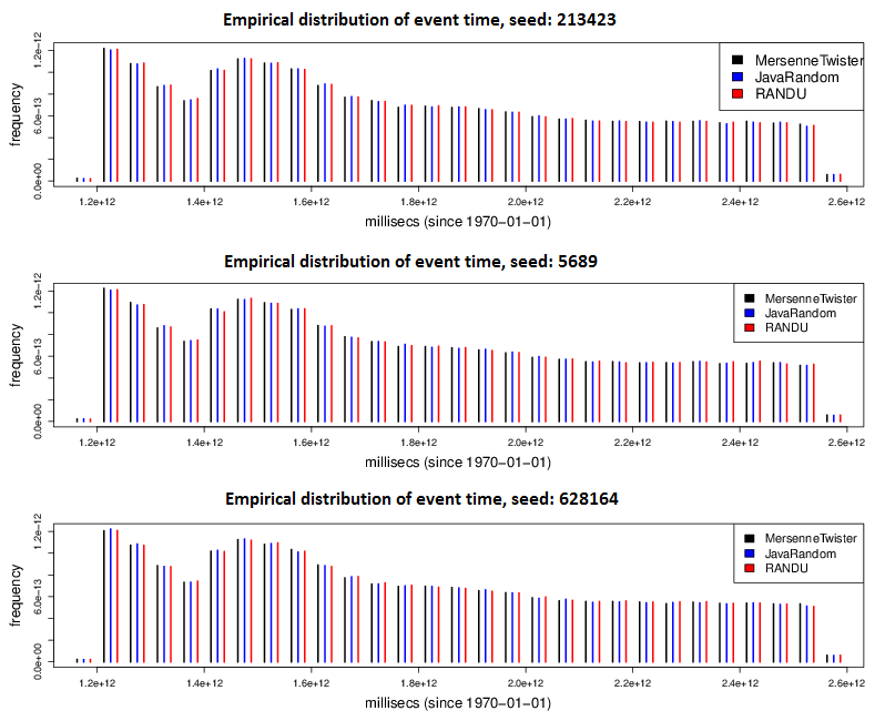
Figure 6. Comparison of empirical event time distributions. - 4.13
- To find out whether potential regularities in the pattern of drawn random variates bias the simulation outcome, we have analyzed the empirical distributions of all events that have occurred within the simulation period. Empirical event distributions have been computed for each random number generator and each selected seed separately. Figure 6 shows the results. In summary, a comparison of the empirical event distributions achieved using the three different PRNGs does not reveal any remarkable differences in the simulation results.
Performance issues
- 4.14
- The performance of M&S software depends on a variety of factors. In this section we focus on the impact of a single sub data structure used by the computation algorithm. Primarily the model is crucial: depending on its structure different data structures or algorithms perform better than others (Jeschke & Ewald 2008). In the subsequent, for our example setting we analyze how well event handling is managed by different data structures. The continuous-time microsimulation models are essentially discrete event models whose computation is based on event queues (see Algorithm 1). In the Mic-Core the event queue is integrated into the computation algorithm using the plug-in mechanism of JAMES II. Therefore, event queues can easily be exchanged for each new computation without the need to modify any code. JAMES II comprises several event queue realizations (Himmelspach & Uhrmacher 2007a). As in our application events have only to be enqueued into and dequeued from an event queue, our review does not comprise any event queue extensions that include requeue operations (which allow to update the time of an already enqueued event). For our experiments we have selected the following four implementations of event queues from JAMES II:
- MList,
- CalendarQueue,
- Heap based, and
- SimpleQueue.
- 4.15
- The MList, the calendar queue, and the heap queue are well-known event queues and are comprehensively described in literature (Brown 1988; Goh & Thng 2003; van Emde Boas et al. 1977). The simple event queue is a data structure that employs an unsorted list to maintain events. In our study it serves as a reference to evaluate the performance of the other queue implementations considered. By experimental evaluation supported by JAMES II we have analyzed which of the listed queues performs best for the example scenario. Figure 7 illustrates the corresponding experiment specification in JAMES II.
- 4.16
- We have executed the experiments on a desktop workstation equipped with two Xeon quad core CPUs, activated hyper threading, deactivated automated CPU overclocking, equipped with 32GB of RAM achieving a Windows Experience index of 7.8 for CPU and memory and Java Sci mark (using Java VM 1.6.0 (64 bit)). We have run each experiment four times to eliminate the impact of further concurrent processes on the machine. In the Mic-Core data collection is done using a file based storage. Any outcome data is kept in memory, and to avoid any side effects, written after a simulation run has been finished. In our experiments we have used the Mersenne Twister as PRNG, initialized with seed 10991.
Example of how to set the MList event queue and the Mersenne Twister PRNG with the seed 10991:

  exp.getParameters().getParameterBlock()
   .addSubBl(ProcessorFactory.class.getName(),
     new ParameterBlock("MicCoreProcessorFactory").
       addSubBl("eventqueue", "MListFactory").
       addSubBlock("RNGGenerator", "MersenneTwisterGeneratorFactory").
         addSubBl("seed", 10991)));
Figure 7. Example of setting experiment parameters. In this exercise the performance of different event queue implementations (MList, CalendarQueue, SimpleQueue, and heap based queue) has been studied. The schema and the code snippet (Java) illustrate how the accordant experiment has been specified. - 4.17
- The subsequent table shows the mean execution times (in seconds) of our experiment setup.
Population size
Event Queue1% 2% 20% 100% MList 4.06 (0.17) 5.17 (0.27) 29.50 (2.59) 134.32 (4.53) HeapEventQueue 4.12 (0.30) 5.32 (0.47) 30.25 (2.08) 145.24 (6.23) CalendarQueue 4.40 (0.31) 6.42 (0.48) 135.66 (1.92) 4101.41 (329.99) SimpleEventQueue 12.60 (0.72) 2210.34 (142.96) NaN NaN - 4.18
- Each experiment has been executed four times. In brackets the standard deviation is given. All values have been rounded to two digits after the decimal comma. The "NaN" notation shows that corresponding runs have been interrupted because of enormously long run times. The times clearly show that the event queue implementation has a considerable impact on the overall runtime. That is, using the "wrong" queue results in a remarkable performance loss. In our setting, the simple event queue performs particularly poor. For the Mic-Core we deem the MList event queue as being the most efficient choice.
- 4.19
- As our experiments have been executed with one model only, we redid experiments with two further models and those confirmed our conclusion.
Demographic microsimulation: some results
- 4.20
- In this section we present only very few findings which can be gained from our example. That is, the analysis conducted from the microsimulation results is far from being exhaustive. The purpose is to give a flavor of the variety of questions and implications that can be studied by means of a demographic microsimulation. A more extensive illustration of the capacities of the Mic-Core can be found elsewhere (Zinn et al. 2009; Ogurtsova et al. 2010). To demonstrate Mic-Core's capabilities we use ten percent of the initial Dutch cohorts. The Mersenne Twister random number generator, initialized with seed 10911, has served as PRNG. Further, we have used the MList event queue to collect events and event times. After a simulation run is completed, Mic-Core stores the information on the simulated life courses in two files: an ASCII file containing the birth dates of all simulated individuals, and an ASCII file containing the dates of transitions and the corresponding destination states for all simulated individuals. These files have a well-defined format, which can be accessed and managed further by arbitrary tools. The format of the output files is comprehensively described in the manual of the Mic-Core (Zinn & Gampe 2011). We have implemented in the statistical environment R a comprehensive palette of instruments in order to evaluate and illustrate the output of a microsimulation run. We call this palette the "post-processor" of the Mic-Core. The post-processor and a corresponding manual can be downloaded at http://www.demogr.mpg.de/cgi-bin/micmac/login.plx. It is freely available.
- 4.21
- At first we use the post-processor to convert the microsimulation output into a format resembling event history data. This format eases further computation. In Figure 8, typical life-courses of four simulated individuals are given, already transformed by the post-processor. Each record describes one event that an individual has experienced during simulation. A record gives an individual's identification number and his/her birth time, the transition date, the transition age, and the state to which the individual has made a transition. The first transition date of individuals who are part of the initial cohorts corresponds to the simulation starting time, and the state to which an individual moves in this case is the initial state. Likewise, the first transition time of a newborn corresponds to his/her birth date and the state to which a newborn moves is the state that he/she occupies at birth. (The assignment of newborns to the state space is comprehensively described in the manual of the Mic-Core.)
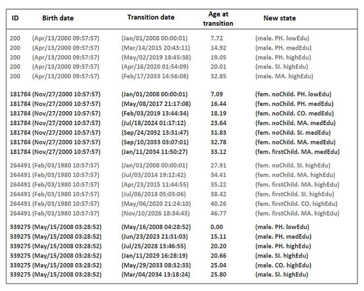
Figure 8. The simulated life-courses of four individuals. The column 'Birth date' gives the birth dates of the individuals, 'Transition date' contains the transition dates, and 'Age at transition' the corresponding transition ages. 'New state' gives the states that individuals enter when they undergo an event; coding: male (male), fem (female), PH (living at parental home), SI (living alone), MA (married), CO (cohabiting), noChild (childess), firstChild (mother of one child), lowEdu (primary school), medEdu (lower secondary school), highEdu (upper secondary or tertiary education). - 4.22
- Using the microsimulation data converted in this way allows easily studying individual life courses. An example is the analysis of life courses that were simulated most frequently. Figure 9 shows the distribution of the transition ages in the most frequently simulated life courses of individuals born in 2000.
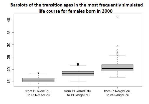
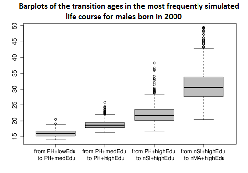
Figure 9. Distribution of the transition ages in the most frequently simulated life course of individuals born in 2000. Females are depicted in the left graph and males are shown in the right graph. The most frequently simulated life course of females and males, respectively, involves that living at parental home (PH) females/males undergo education until reaching the highest level (from 'lowEdu' over 'medEdu' to 'highEdu'). Subsequently, they leave parental home to live alone (nSI). Males continue by marrying for the first time (nMA), while females more frequently stay single. - 4.23
- We find that the life course that ranges on the second position of the list of the most frequently simulated life courses concerns individuals with only primary school education (see Figure 10): after having finished primary school ('lowEdu'), these individuals leave the parental home ('PH') to stay alone ('SI'), and to marry ('MA') after a short while. After having married, females quickly start their fertility carrier ('firstChild','secondChild').
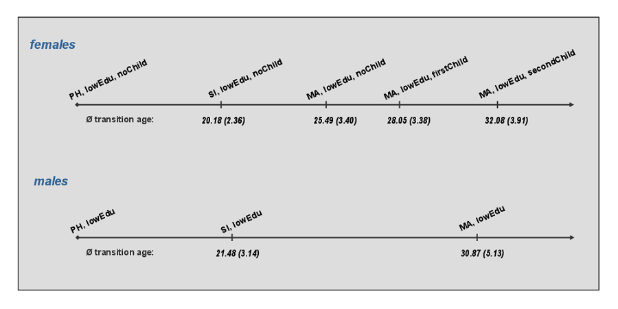
Figure 10. Life-courses that range on the second position of the most frequently simulated life-courses for females and males. The average age of each event is given below the respective event (the corresponding standard derivations are added in parenthesis); coding: PH (living at parental home), SI (living alone), MA (married), lowEdu (primary school), noChild (childess), firstChild (mother of one child), secondChild (mother of two children). - 4.24
- In a further step, we analyze the frequency distribution of the states that individuals who are born in 1980 occupy at the beginning of each calendar year. We are interested how this frequency distribution changes over time. Figure 11 depicts the results of our analysis. At first glance it might be surprising that over simulation time many women marry, either after having been single before or subsequent to cohabitation. If we mind that at simulation starting time the women who are born in 1980 are between 27 and 28 years old, the result is not very surprising. The males who are born in 1980 show a similar behavior.
- 4.25
- A highly topical research question that could be studied with our setting is the question of mechanisms behind male and female family differences and their future implications for society. This is particularly interesting with respect to the availability of informal carers to take on a caring role at older ages or in case of disability. We find that men seem mostly to stay with their first marriage, while women undergo more often higher order marriages (second, third, etc. marriages). This result suggests that women tend to have wider access to informal carers than men.
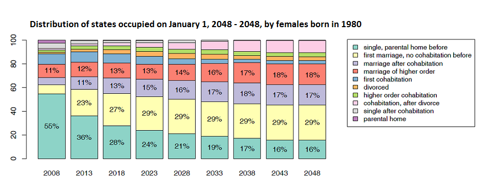
Figure 11. Frequency distribution of states that individuals who are born in 1980 occupy at the beginning of each fifth calendar year.
Summary: Lessons learned
- 5.1
- The development team of the Mic-Core consisted of two persons: one acting as the chief developer (P1) of the Mic-Core and the other one being the assistant with in depth knowledge about JAMES II (P2). Due to the close partnership and the usage of a common repository for exchange any problems encountered have been resolved in a relatively short time (often in less than an hour and at most a day). Using a library or a framework always imposes some overhead: the user has to understand the way the designers of the library/framework built it and how he/she can make use of the functionality provided in there. This discrepancy between the functionality wanted and the functionality provided by JAMES II had been the major problem in the beginning of the project. In line therewith, in the early development stages of the Mic-Core the designer P1 faced the challenge to overview and to comprehend this extensive set of functionality. The extensive usage of interfaces and the consequent employment of the plug-in concept throughout the framework make the learning curve quite steep: once the user understands how it works, it is the same for all the rest.
- 5.2
- The core development of the Mic-Core was done after twenty weeks - ending with fully-fledged M&S software - principally supporting the principles and techniques described in (Himmelspach 2009). During the main realization phase of the Mic-Core, P1 has learned to appreciate the benefits of using a framework. One example is the possibility to try alternative event queue implementations. In summary, for the Mic-Core the following functionalities provided by JAMES II have been reused so far:
- the experimentation layer (experiment definition and automated execution; replications),
- the data sinks (storages),
- random number generation/distributions,
- random sampling methods,
- the event queues, and
- some further utility methods.
- 5.3
- For the designers of the Mic-Core using JAMES II meant to considerably save development costs because there was no need to build existing functionalities newly. They could profit from the high expert M&S knowledge that is included in JAMES II, and implementation work done by others.
- 5.4
- In addition, due to the huge number of state transitions to be recorded while the simulation is being executed, it turned out that besides efficient data structures and algorithms the need for efficient data sinks (and alternative storages) is very high. In the beginning of the project the data sinks had not been optimized sufficiently and caused a significant slowdown of the computation. This insight started new research on further optimizations of the data recording process (Himmelspach et al. 2010).
- 5.5
- The experiences we made during this endeavor are presented in the subsequent summary.
P1 P2 The development of Mic-Core was possible in a relatively short time. Good documentation needed - otherwise "too" many problems will prevent usage. Not all software development needs had been known in advance. Framework had been usable as expected. The requirements of the project have been fulfilled. Framework provided more than needed/wanted but some of these things proved to be beneficial later on. Potential impacts of implementations can be checked which otherwise would have (most likely) remained unexplored. Good argumentation for solutions required (e.g., why strict separation of concerns). It was worth investing the time to get acquainted with JAMES II. Release management required to decouple development of the framework from the development of software based on it. To use a framework helps to stay up to date - improvements of algorithms/data structures used come for free. Usage scenario: Framework (software based on it) as tool in a pipes and filter chain. Using a framework was helpful as more time was available for validation. Data sinks can make up a huge part of the overall runtime. Differing definitions of basic terms - barrier for reuse. - 5.6
- We can state that using a framework for M&S software to build new M&S software products can significantly ease the development. Such processing reduces the costs and makes it much easier to get a mature software product providing support for a variety of state of the art techniques in the end. The time to be invested to get in touch with the framework seems to be more than compensated, if we account for the benefit that we take from reusing well-tested software components. In conclusion, we deem it not being advisable to start the development of software products for M&S from scratch. Too many M&S techniques might be required. In the beginning developers might not even be aware of all functionality needed, which might lead to intensive refactorings of the software developed so far later on. Finally, software validation and maintenance seems to be intractable for small teams.
Outlook
- 6.1
- The modeling and simulation framework JAMES II offers several features that are useful for further developments of the MicMac microsimulation tool and to build up extensions of it. JAMES II provides workflow support for executing more sophisticated experiments than the ones described, like optimization experiments (Himmelspach et al. 2010). Furthermore, to borrow functionality from other software JAMES II permits interfaces, e.g., to the statistical environment R. It allows different parameterizations of the data sinks used/usable, and the GUI of JAMES II can be used as a framework for the creation of a more specialized GUI. JAMES II's toolbox holds techniques for automated algorithm selection, parallel jobs, and parallel replications. For example, the costs for adding support for parallel replications in Mic-Core are very low: just a single parameter has to be exchanged in the experimentation layer used. Filling a second parameter, a so called master server can be used to execute the parallel replications on remote computers. Also in another direction JAMES II's experimentation layer offers a considerable facilitation: For population projections, assumptions about (possible) prospective developments have to be made. One way to describe such developments is the use of if-then scenarios, which allow demonstrating the consequences of hypothetical conditions, such as different policies. To obtain a comprehensive picture of possible future population dynamics, a microsimulation has to be parameterized accordingly; i.e., for each envisaged "if-then scenario" a set of prospective transition rates has to be prepared. It is challenging, however, to formulate options about changes in the future as changes of particular model parameters. Usually, experts asked for their assessment estimate prospective parameter values only roughly (Lutz 2009). That is, modelers are often confronted with statements like: in 2050 the total fertility rate in Germany ranges between 1.2 and 1.5. Such statements require running a huge number of microsimulation models and to evaluate an immense amount of microsimulation output. The experimentation layer of JAMES II allows automatically performing such an endeavor.
- 6.2
- When performing population projections, simulated population totals are often claimed to match benchmark values of official statistics (Harding 2007). That is, microsimulation output has to be aligned to external projections of aggregated or group variables. This claim usually requires to adapt the specification of the considered microsimulation model, for example, to adapt the input transition rates. The Mic-Core does not account for this need. JAMES II can be applied to overcome this drawback: it allows to thoroughly exploring huge parameter spaces in short time, e.g., by using concepts of experimental model validation (Leye & Uhrmacher 2012).
- 6.3
- Currently, the Mic-Core produces synthetic life courses of all members of a virtual population which can later be analyzed by using, e.g., the post-processor of the MicMac software (Gampe & Zinn 2011). Recently, an instrumentation language has been integrated into JAMES II that allows specifying declaratively what information about simulation runs shall be collected (Helms et al. 2012). By using the language, instrumenters are assigned to models and specific variables of a model can be observed. Depending on certain properties, variable values can be sampled according to certain temporal patterns. Aggregates can be calculated on the fly. Such functionality allows for example to only observe population subgroups of interest (such as childless women or people older than sixty). Storing synthetic life courses of all population members is not any longer necessary. Consequently, the overall amount of memory required to store the microsimulation output can be reduced. Furthermore, using such a language makes parts of any microsimulation post-processing software obsolete.
- 6.4
- Simulating individual life courses independently is the usual starting point for demographic microsimulations, but realistic population modeling cannot get away from considering so called 'linked lives'. People cohabit or marry, have children and live in families; and this environment has an impact on their demographic behavior. This implies that some individual demographic events require that other individuals are linked to a person, and the relationship between linked individuals may modify their future behavior (i.e., the behavioral model describing concordant life-courses). Due to its rigid structure the Mic-Core implementation referred to here, however, hampers extending the MicMac microsimulation accordingly. Therefore, using JAMES II for the MicMac microsimulation also a DEVS (discrete event specification) model has been specified and implemented (Zinn et al. 2010). The DEVS formalism offers all the functionalities that are necessary to formulate population dynamics in the required way. First steps towards the inclusion of linked lives have already been performed (Zinn 2012).
- 6.5
- As soon as a micro model accounts for interaction and linkage patterns between individuals - besides the micro level of a population - also a group level becomes emergent, the meso level. Here interacting individuals are grouped according to the type of interaction, e.g, into households, families, firms, or even party membership. Generally, complex dynamic systems, like populations, can be specified at three different structural levels: micro, meso, and macro. The latter gives the conditions under which the target system is considered: If a human population is studied, macro conditions are, e.g., the political and the economic system, distinct policies, the taxation and benefit system, the environmental conditions etc. In conjunction with microsimulations the concept of meso levels has de facto never been described as such. Also the dynamics of macro structures, like a changing political system, are not modeled - usually the macro-level is measured as aggregates of individual attributes (Gilbert & Troitzsch 2008). A feedback from the individual behavior on the macro condition is hence not foreseen. In order to make a step towards a multi-level approach, a set of challenges have to be met to specify and implement a demographic microsimulation that allows interaction among individuals, and between individuals and their environment. In particular, a suitable and approachable simulation development bench is needed. JAMES II fulfills these requirements. It exhibits a highly perspicuous work bench; new models and simulators can be implemented on a plug-in basis, and therefore be easily re-used and exchanged. A multi-level simulation very likely becomes a very complex system requiring extensive facilities for data storage, statistical analysis, and visualization modules. In this direction JAMES II offers many useful features.
Appendix: Transition rates used to specify the model
- 7.1
- In paragraphs 4.1 - 4.25 we describe an application for a population which closely resembles the contemporary Netherlands. In this appendix we present the age-profiles of the transition rates used in this application.
- 7.2
- Transition rates related to changes in living arrangement and marital status are given in Figures 12, 13, 14, 15, 16 (for females), and also in Figures 19, 20, and 21 (for males). Figure 17 and Figure 18 top show the birth rates of females. While we assume that during simulation transition rates for changing the marital status and parity vary with age, they are held constant over calendar time. Figure 18 bottom shows the transition rates of females to a higher level of educational attainment, while Figure 21 bottom shows the corresponding rates for males. Furthermore, the following assumptions were made to simplify the model and to reduce the number of required transition rates.
- For both sexes the rates to leave parental home do not depend on the presence of children.
- Additionally, for males the transition rates to leave parental home because of marriage are independent of their educational attainment.
- Divorce rates are independent of the marriage order.
- Females move into cohabitation after living alone, once they have left parental home, independent of the presence of children.
- For both sexes the transition rates from cohabitation to marriage do not depend on the partnership order.
- The propensity to move into cohabitation after a previous partnership is independent of the type of the former partnership (marriage or cohabitation).
- For both sexes the risk to split up is independent of the partnership order and the presence of children.
- Rates that describe a transition to parity three or more do not depend on the marital status or the living arrangement of the woman.
- The probability to change the educational attainment is independent of marital status and living arrangement, and also of the presence of children.
- 7.3
- Mortality rates are given in Figure 22.
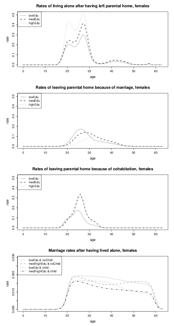
Figure 12. Transition rates of females who leave parental home and marriage rates of females (by educational attainment); lowEdu: only primary school, medEdu: lower secondary school, highEdu: upper 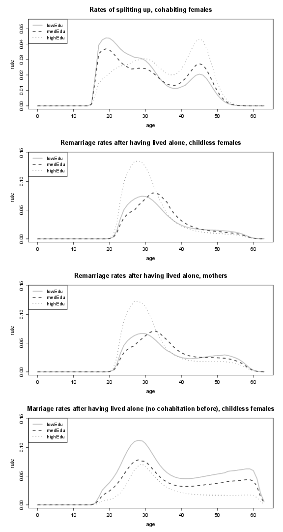
Figure 13. Rates of splitting up, marriage and remarriage rates of females (by educational attainment); lowEdu: only primary school, medEdu: lower secondary school, highEdu: upper secondary or tertiary education. 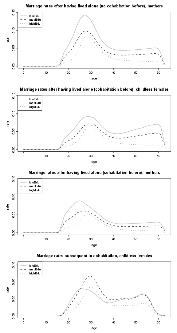
Figure 14. Marriage rates of females (by educational attainment); lowEdu: only primary school, medEdu: lower secondary school, highEdu: upper secondary or tertiary education. 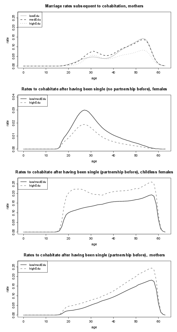
Figure 15. Marriage rates of females (by educational attainment), part 2; lowEdu: only primary school, medEdu: lower secondary school, highEdu: upper secondary or tertiary education. 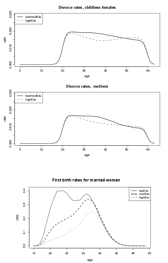
Figure 16. Divorce rates of females, and birth rates (by educational attainment); lowEdu (only primary school), medEdu (lower secondary school), highEdu (upper secondary or tertiary education). 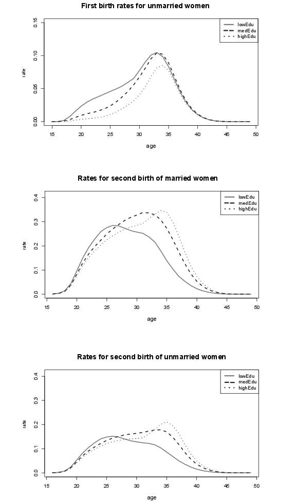
Figure 17. Birth rates by educational attainment; lowEdu: only primary school, medEdu: lower secondary school, highEdu: upper secondary or tertiary education. 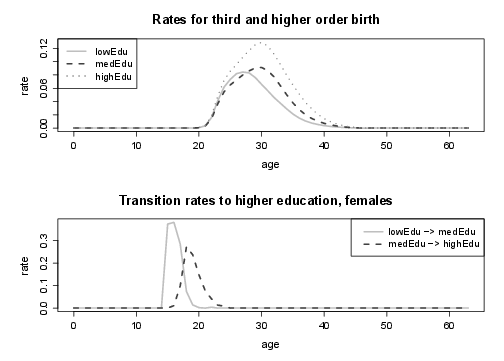
Figure 18. Birth rates by educational attainment and transition rates to higher educational attainment; lowEdu: only primary school, medEdu: lower secondary school, highEdu: upper secondary or tertiary education. 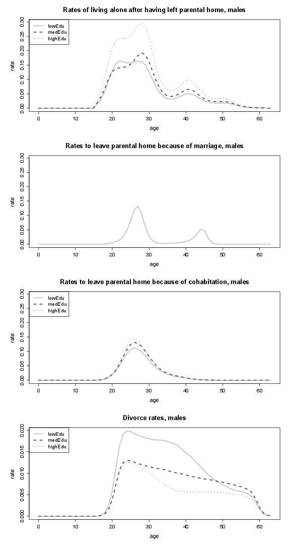
Figure 19. Rates to leave parental home and divorce rates of males (by educational attainment); lowEdu: only primary school, medEdu: lower secondary school, highEdu: upper secondary or tertiary education. 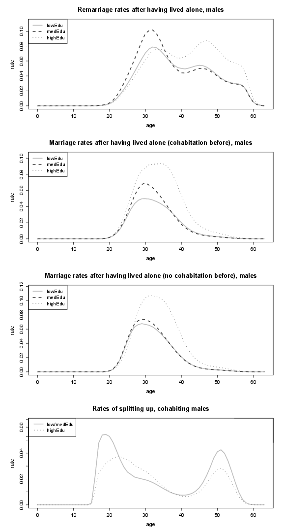
Figure 20. Marriage and remarriage rates of males, and rates of splitting up (by educational attainment); lowEdu: only primary school, medEdu: lower secondary school, highEdu: upper secondary or tertiary education. 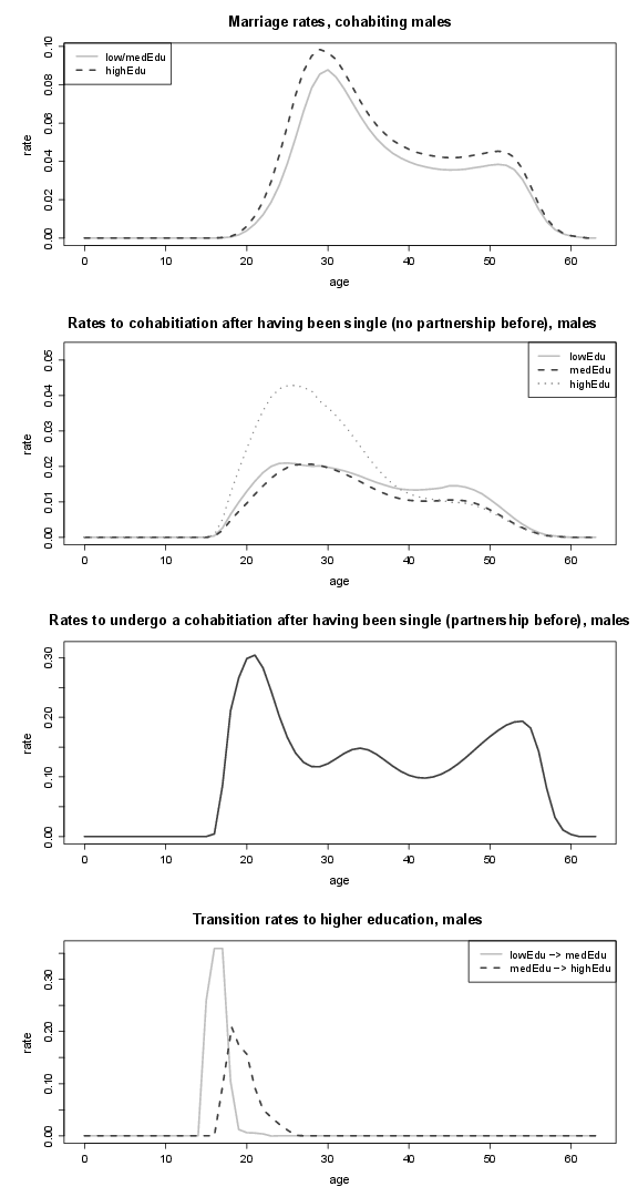
Figure 21. Marriage rates of males and rates of males to cohabitation (by educational attainment), as well as transition rates to higher educational attainment; lowEdu: only primary school, medEdu: lower secondary school, highEdu: upper secondary or tertiary education. 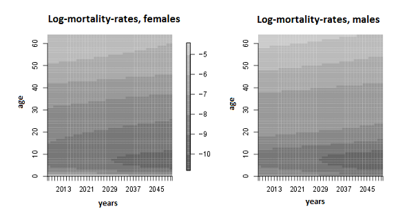
Figure 22. Image plot of log-mortality rates of females and males.
Acknowledgements
- This research has been founded by the EU project MicMac and is based upon the CoSA project supported by the DFG (German Research Foundation).
References
-
ANDERSEN, P. & Keiding, N. (2002). Multi-state models for event history analysis. Statistical Methods in Medical Research, 11(2), 91-115. [doi:10.1191/0962280202SM276ra]
BARTHOLOMEW, D. J. (1973). Stochastic Models for Social Processes. John Wiley & Sons, 2nd ed.
BROWN, R. (1988). Calendar queues: a fast 0(1) priority queue implementation for the simulation event set problem. Commun. ACM, 31(10), 1220-1227. [doi:10.1145/63039.63045]
CLARK, G., Courtney, T., Daly, D., Deavours, D., Derisavi, S., Doyle, J., Sanders, W. & Webster, P. (2001). The Möbius modeling tool. In 9th international Workshop on Petri Nets and Performance Models (PNPM'01). IEEE. [doi:10.1109/PNPM.2001.953373]
COLLIER, N. & North, M. (2011). Repast sc++: A platform for large-scale agent-based modeling. In W. Dubitzky, K. Kurowski & B. Schott (Eds.), Large-Scale Computing Techniques for Complex System Simulations. Wiley.
EDMONDS, B. & Hales, D. (2003). Replication, replication and replication: some hard lessons from model alignment. Journal of Artificial Societies and Social Simulation, 6(4) 11. https://www.jasss.org/6/4/11.html
EUROSTAT (2012). http://epp.eurostat.ec.europa.eu/portal/page/portal/statistics/ (accessed September 2012).
EWALD, R., Himmelspach, J., Jeschke, M., Leye, S. & Uhrmacher, A. (2010). Flexible experimentation in the modeling and simulation framework JAMES II - implications for computational systems biology. Briefings in Bioinformatics, 11(3), 290-300. [doi:10.1093/bib/bbp067]
EWALD, R., Himmelspach, J., Jeschke, M., Leye, S. & Uhrmacher, A. M. (2009). Performance issues in evaluating models and designing simulation algorithms. In Proceedings of the 2009 International Workshop on High Performance Computational Systems Biology. IEEE CPS. [doi:10.1109/HiBi.2009.16]
GALAN, J. & Izquierdo, L. (2005). Appearances can be deceiving: lessons learned re-implementing Axelrod's 'evolutionary approach to norms' Journal of Artificial Societies and Social Simulation, 8(3) 2. https://www.jasss.org/8/3/2.html.
GALLER, H. (1997). Discrete-time and continuous-time approaches to dynamic microsimulation (reconsidered). Tech. rep., NATSEM - National Centre for Social and Economic Modelling, Faculty of Management, University of Canberra.
GAMPE, J., Ogurtsova, E. & Zinn, S. (2010). The MicMac Pre-Processor. MPIDR, Rostock. http://www.demogr.mpg.de/cgi-bin/micmac/login.plx.
GAMPE, J. & Zinn, S. (2007). Description of the microsimulation model. Technical report, MicMac project, MPIDR, Rostock. http://www.nidi.nl/Content/NIDI/output/micmac/micmac-d8b.pdf. Archived at: http://www.webcitation.org/6Cf1UNmEs.
GAMPE, J. & Zinn, S. (2011). The MicMac Post-Processor. MPIDR, Rostock. http://www.demogr.mpg.de/cgi-bin/micmac/login.plx.
GILBERT, N. & Troitzsch, K. (2008). Simulation for the Social Scientist, chap. Multilevel simulation models. Open University Press, pp. 100-129.
GOH, R. & Thng, I.-J. (2003). MList: An efficient pending event set structure for discrete event simulation. International Journal of Simulation - Systems, Science & Technology, 4(5-6), 66-77.
GRIBBLE, S., Hicks, C. & Rowe, G. (2003). The LifePaths microsimulation model. Paper presented at the International Microsimulation Conference on Population Ageing and Health: Modelling Our Future, Canberra, 7-12 December. Available at: www.natsem.canberra.edu.au.
HANNAY, J., Langtangen, H., MacLeod, C., Pfahl, D., Singer, J. & Wilson, G. (2009). How do scientists develop and use scientific software? In Proceedings of the SECSE. IEEE. [doi:10.1109/secse.2009.5069155]
HARDING, A. (2007). Challenges and opportunities of dynamic microsimulation modelling. Plenary paper presented to the 1st General Conference of the International Microsimulation Association, Vienna, 21 August 2007.
HELLEKALEK, P. (1998). Good random number generators are (not so) easy to find. Mathematics and Computers in Simulation, 46, 485-505. [doi:10.1016/S0378-4754(98)00078-0]
HELMS, T., Himmelspach, J., Maus, C., Röwer, O., Schützel, J. & Uhrmacher, A. (2012). Toward a language for the flexible observation of simulations. In C. Laroque, J. Himmelspach, R. Pasupathy, O. Rose, & A. M. Uhrmacher (Eds.), Proceedings of the 2012 Winter Simulation Conference. Piscataway, New Jersey: Institute of Electrical and Electronics Engineers, Inc. [doi:10.1109/WSC.2012.6465073]
HIMMELSPACH, J. (2009). Toward a collection of principles, techniques, and elements of simulation tools. In: Proceedings of the First International Conference on Advances in System Simulation (SIMUL 2009), Porto, Portugal. IEEE Computer Society. [doi:10.1109/SIMUL.2009.19]
HIMMELSPACH, J. (2012). Tutorial on how to build M&S software based on reuse. In C. Laroque, J. Himmelspach, R. Pasupathy, O. Rose, & A. M. Uhrmacher (Eds.), Proceedings of the 2012 Winter Simulation Conference. Piscataway, New Jersey: Institute of Electrical and Electronics Engineers, Inc. [doi:10.1109/WSC.2012.6465306]
HIMMELSPACH, J., Ewald, R., Leye, S. & Uhrmacher, A. (2010). Enhancing the scalability of simulations by embracing multiple levels of parallelization. In Proceedings of the 2010 International Workshop on High Performance Computational Systems Biology. IEEE CPS. [doi:10.1109/pdmc-hibi.2010.17]
HIMMELSPACH, J., Ewald, R. & Uhrmacher, A. (2008). A flexible and scalable experimentation layer for JAMES II. In: S. Mason, R. Hill, L. Moench, O. Rose, T. Jefferson & J. W. Fowler (Eds.), Proceedings of the 2008 Winter Simulation Conference. Piscataway, New Jersey: Institute of Electrical and Electronics Engineers, Inc. http://www.informs-sim.org/wsc08papers/099.pdf. [doi:10.1109/WSC.2008.4736146]
HIMMELSPACH, J. & Uhrmacher, A. (2007a). The event queue problem and PDEVS. In Proceedings of the DEVS Integrated M&S Symposium. Norfolk, VA: SCS.
HIMMELSPACH, J. & Uhrmacher, A. (2007b). Plug'n simulate. In Proceedings of the 40th Annual Simulation Symposium. IEEE Computer Society. [doi:10.1109/anss.2007.34]
HIMMELSPACH, J. & Uhrmacher, A. (2009). What contributes to the quality of simulation results? In L. H. Lee, M. E. Kuhl, J. W. Fowler & S. Robinson (Eds.), Proceedings of the 2009 INFORMS Simulation Society Research Workshop. University of Warwick, Coventry, U.K.: INFORMS Simulation Society.
IMPICCIATORE, R. & Billari, F. (2011). MAPLES: A general method for the estimation of age profiles from standard demographic surveys (with an application to fertility). De, 24(29), 719-748. [doi:10.4054/demres.2011.24.29]
JESCHKE, M. & Ewald, R. (2008). Large-scale design space exploration of SSA. In Computational Methods in Systems Biology, International Conference, CMSB 2008, Rostock, Germany, October 12-15, 2008, Proceedings, vol. 5307 of Lecture Notes in Computer Science. Berlin/Heidelberg: Springer. [doi:10.1007/978-3-540-88562-7_17]
JOHN, M., Lhoussaine, C., Niehren, J. & Uhrmacher, A. (2010). The attributed pi-calculus with priorities. In Transactions on Computational Systems Biology XII (pp. 13-76), vol. 5945 of Lecture Notes in Computer Science. Berlin/Heidelberg: Springer.
KC, S., Barakat, B., Goujon, A., Skirbekk, V. & Lutz, W. (2010). Projection of populations by level of educational attainment, age and sex for 120 countries for 2005-2050. Demographic Research, 22(15), 383-472. [doi:10.4054/DemRes.2010.22.15]
KLÜGL, F. & Puppe, F. (1998). The multi-agent simulation environment SeSAm. In H. K. Büning (Ed.), Proceedings des Workshops Simulation in Knowledge-based Systems, vol. tr-ri-98-194 of Reihe Informatik. Paderborn: Universität Paderborn.
KURKOWSKI, S., Camp, T. & Colagrosso, M. (2005). MANET simulation studies: The incredibles. ACM SIGMOBILE Mobile Computing and Communications Review, 9(4), 50-61. [doi:10.1145/1096166.1096174]
L'ECUYER, P. & Hellekalek, P. (1998). Random number generators: Selection criteria and testing. In Random and Quasi-Random Point Sets (pp. 223-266), vol. 138 of Lecture Notes in Statistics. Berlin/Heidelberg: Springer.
LEE, E. (2003). Overview of the ptolemy project. Technical Memorandum UCB/ERL M03/25, University of California, Berkeley, CA, 94720, USA.
LEYE, S. & Uhrmacher, A. (2012). A flexible and extensible architecture for experimental model validation. In 3rd International ICST Conference on Simulation Tools and Techniques, vol. 65. Malaga, Spain: ICST/IEEE.
LUTZ, W. (2009). Toward a systematic, argument-based approach to defining assumptions for population projections. Interim Report IR-09-037, International Institute for Applied Systems Analysis, Austria.
MARSAGLIA, G. (1968). Random numbers fall mainly in the planes. Proceedings of the National Academy of Science, 61(1), 25-28. [doi:10.1073/pnas.61.1.25]
MAUS, C., Rybacki, S. & Uhrmacher, A. (2011). Rule-based multi-level modeling of cell biological systems. BMC Systems Biology, 5(166). [doi:10.1186/1752-0509-5-166]
MAYER, K. & Tuma, N. (eds.) (1990). Event History Analysis in Life Course Research. University of Wisconsin Press.
MERALI, Z. (2010). … why scientific programming does not compute. Nature, 467, 775-777. [doi:10.1038/467775a]
MINAR, N., Burkhart, R., Langton, C. & Askenazi, M. (1996). The SWARM simulation system: A toolkit for building multi-agent simulations. Technical report, Santa Fe Institute.
MOSS, S., Gaylard, H., Wallis, S. & Edmonds, B. (1998). SDML: a multi-agent language for organizational modelling. Computational and Mathematical Organization Theory, 4(1), 43-69. [doi:10.1023/A:1009600530279]
NIDI (2011). MicMac homepage. http://www.nidi.nl/smartsite.dws?lang=UK&ch=NID&id=25014. Archived at: http://www.webcitation.org/6Cf4eJuiF.
OGURTSOVA, E., Gampe, J. & Zinn, S. (2010). Practical population forecasting by microsimulation: application of the MICMAC software. In Conference of European Statisticians, Joint Eurostat/UNECE Work Session on Demographic Projections (28-30 April 2010, Lisbon, Portugal), Item 12 - Stochastic techniques for demographic projections. United Nations Statistical Commission and Economic Comission for Europe, Statistical Office of the European Union (EUROSTAT).
ORCUTT, G. (1957). A new type of socio-economic system. Review of Economics and Statistics, 39(2), 116-123. [doi:10.2307/1928528]
ORCUTT, G., Greenberger, M., Korbel, J. & Rivlin, A. (1961). Microanalysis of Socioeconomic Systems: A Simulation Study. New York: Harper & Row.
PARK, A. & Fujimoto, R. (2007). A scalable framework for parallel discrete event simulations on desktop grids. In: Proceeding GRID '07 Proceedings of the 8th IEEE/ACM International Conference on Grid Computing, IEEE Computer Society Washington, 185-192. [doi:10.1109/grid.2007.4354132]
PAWLIKOWSKI, K., Jeong, H.-D. & Lee, J.-S. (2002). On credibility of simulation studies of telecommunication networks. Communications Magazine, IEEE, 40(1), 132-139. [doi:10.1109/35.978060]
PERUMALLA, K. (2005). μsik: a micro-kernel for parallel/distributed simulation systems. In ACM/IEEE/SCS Workshop on Parallel and Distributed Simulation (PADS). Monterey, CA: IEEE Computer Society Press.
PRESS, W., Teukolsky, S., Vetterling, W. & Flannery, B. (2007). Numerical Recipes - The Art of Scientifc Computing. Cambridge University Press, 3rd ed.
RIBAULT, J., Dalle, O. & Himmelspach, J. (2009). Design considerations for M&S software. In M. D. Rossetti, R. R. Hill, B. Johansson, A. Dunkin & R. G. Ingalls (Eds.), Proceedings of the 2009 Winter Simulation Conference. IEEE Computer Society. Invited paper.
RUBINSTEIN, R. & Kroese, D. (2008). Simulation and the Monte Carlo Method. Series in Probability and Statistics. Wiley, 2nd ed.
SOMMERVILLE, I. (2007). Software Engineering. Addison-Wesley, 8th ed.
STATISTICS CANADA (2011). Modgen version 9.0.10: Developer's guide. http://www.statcan.gc.ca/microsimulation/modgen/modgen-eng.htm (accessed September 2012).
STEINIGER, A., Krüger, F. & Uhrmacher, A. M. (2012). Modeling and simulation of agents and their environment using multi-level-devs. In C. Laroque, J. Himmelspach, R. Pasupathy, O. Rose, & A. M. Uhrmacher (Eds.), Proceedings of the 2012 Winter Simulation Conference. Piscataway, New Jersey: Institute of Electrical and Electronics Engineers, Inc. [doi:10.1109/WSC.2012.6465113]
VAN EMDE BOAS, P., Kaas, R. & Zijlstra, E. (1977). Design and implementation of an efficient priority queue. Mathematic Systems Theory, 10, 99-127. [doi:10.1007/BF01683268]
VAN IMHOFF, E. (1990). The exponential multidimensional demographic projection model. Mathematical Population Studies, 2(3), 171-181. [doi:10.1080/08898489009525305]
WILLEKENS, F. (2009). Continuous-time microsimulation in longitudinal analysis. In A. Zaidi, A. Harding & P. Williamson (Eds.), New Frontiers in Microsimulation Modelling (pp. 353-376). Ashgate, Farnham, Surrey, UK. (Book released during 2nd International Microsimulation Conference, Ottawa, June 2009).
WOLF, D. (1986). Simulation methods for analyzing continuous-time event-history models. Sociological Methodology, 16, 283-308. [doi:10.2307/270926]
ZINN, S. (2012). A mate-matching algorithm for continuous-time microsimulation models. International Journal of Microsimulation, 5(1), 31-51.
ZINN, S. & Gampe, J. (2011). The MicMacCore. MPIDR, Rostock. http://www.demogr.mpg.de/cgi-bin/micmac/login.plx.
ZINN, S., Gampe, J., Himmelspach, J. & Uhrmacher, A. (2010). A DEVS model for demographic microsimulation. In: Spring Simulation Multi-Conference - Symposium on Theory of Modeling & Simulation - DEVS Integrative M&S Symposium (DEVS). San Diego: SCS Publishing House. [doi:10.1145/1878537.1878689]
ZINN, S., Himmelspach, J., Gampe, J. & Uhrmacher, A. (2009). Mic-Core: A tool for microsimulation. In M. D. Rosetti, R. R. Hill, B. Johansson, A. Dunkin & R. G. Ingalls (Eds.), Proceedings of the 2009 Winter Simulation Conference. Piscataway, NJ: IEEE. [doi:10.1109/WSC.2009.5429424]