
 Abstract
- Export firms have better performance than firms that do not export, the so-called exporter premia: exporters are larger, they are relatively more capital and skill intensive, exporters have higher productivity (Bernard et al. 2007a; Bernard et al. 2005). The better performance of exporters may be the result of a self-selection effect: only the most competitive firms are able to enter foreign markets (ex-ante self-selection). On the other hand, exporting may improve firm performance (ex-post effect). Differences between exporters and non-exporters may have a significant impact on aggregate welfare and growth; in particular, disentangling the importance of the ex-ante effect from the ex-post effect may be useful for designing public policies (Bernard & Jensen 1999). The economic approach based on the Melitz (2003) model analyzes the exporter premia using monopolistic competition markets with firm heterogeneity in terms of a given distribution of firm productivity. This paper presents an agent based simulation of a monopolistic competition market in which firm heterogeneity is an emerging pattern of firms' choices and interactions, conceiving productivity growth as the results of firms' individual innovative efforts. The model is able to replicate the better performance of exporters, stressing the importance of decision-making processes and learning capabilities of firms in determining both the ex-ante and the ex-post effects.
- Keywords:
- International Trade, Agent Based Model, Firm Heterogeneity
Introduction
- 1.1
-
There is strong empirical evidence that export firms have a better performance than firms that do not export (exporter premia): exporters are larger, they are relatively more capital and skill intensive, they present higher total factor productivity and higher value added per worker (Feenstra 2003; Bernard et al. 2007a; Bernard et al. 2005).
The exporter premia may be the result of a self-selection effect: only the most competitive firms are able to export because only these firms can overcome fixed costs to enter foreign market (building a commercial network abroad, adapting goods and services to foreign standard and tastes etc..) and variable costs of exporting as transport costs and travel assurance expenditures (Roberts & Tybout 1997; Bernard & Jensen 2004).
On the other hand, exporting may improve firm performance for multiple reasons: firms may access foreign knowledge and technologies (technological spillovers), exporting may increase sales opportunities and, therefore, disposable resources. Moreover, export firms may become more innovative in order to sustain international competition (Aw et al. 2000).
- 1.2
-
Differences between exporters and non-exporters may affect welfare from both static and dynamic perspectives. For instance, if exporters have higher productivity, liberalization measures may increase the aggregate level of productivity because export firms (from the home country and from abroad) may reduce the market share of less competitive firms which do not export. Moreover, higher aggregate productivity may be translated into lower average prices for consumers. Furthermore, if productivity increases when a firm becomes an exporter (ex-post effect), fostering firms to enter foreign markets may be a valid public policy (Acemoglu 2009). However, if the exporter premia is almost exclusively the result of a self-selection effect, public measures that foster exporting may be ineffective and even dangerous (Bernard & Jensen 1999).
Several empirical studies have tried to disentangle the ex-ante self-selection effect from the ex-post effect, they have found robust evidence of the presence of
the self-selection effect while the ex-post effect is less evident.1
- 1.3
-
The economic theory approach based on the Melitz (2003) model analyzes the differences between exporters and non-exporters using a monopolistic competition model with firm heterogeneity in terms of productivity differences among firms, according to a given distribution of firm productivity.2Assuming the presence of (sunk) fixed and variable costs of exporting, the Melitz (2003) model is able to reproduce the exporter premia through the ex-ante self-selection effect: firms with high productivity are able to pay the fixed and variable costs of exporting and, thus, they enter the foreign market. Considering a given distribution of firm productivity the Melitz (2003) model can not deal with the ex-post effect. In fact, the ex-post effect implies productivity growth for firms that enter the foreign market, leading to changes of the firm productivity distribution through time, which may be analyzed by means of a dynamic approach, treating productivity improvements as endogenous.
Starting from a given ex-ante distribution of productivity, the Costantini & Melitz (2007), Bustos (2011) and Burstein & Melitz (2011) models endogenize technological dynamics into the Melitz (2003) framework. These two models are able to analyze the interaction between export decisions and innovative choices in different international trade scenarios.
For instance, on the other hand, in a static framework the Manasse & Turrini (2001) and
the Yeaple (2005) model derive the heterogeneity of the productivity level of firms from the heterogeneity of workers' skills or entrepreneurial ability.
- 1.4
-
The model presented in this paper aims
at analyzing firm heterogeneity as an emergent result of the dynamic combination of exporting and innovation decisions. At the beginning
of the simulations firms have the same level of productivity and size, firms choices
and interactions lead to the differentiation of productivity levels.
The model is based on a two country monopolistic competition market, with initial fixed cost and constant unit cost of exporting. Firms are profit oriented and their choices are the result of a bounded rationality decision process, following a basic reinforcement learning algorithm (Tesfatsion 2005; Roth & Erev 1993) for making choices regarding: selling prices, production capacity, investment in research (for process innovations to increase productivity) and the decision to export or not.
- 1.5
-
The model is able to replicate the better performance of exporters, reproducing both the ex-ante self-selection and the ex-post effects. The results of the simulations suggest that the fixed cost of exporting and the firms' reinforcement learning process lead to the emergence of the ex-post effects, without assuming the presence of higher knowledge spillovers for exporters. In fact, the ex-post effect might be partly related to the firms' learning process: firms that implemented better investment and price strategies are those firms that could be able to enter the foreign market. After starting to export, thanks also to the increased market opportunities, firms might continue to follow the virtuous competitive strategies which allowed them to become exporters, increasing the performance gap with firms that do not export.
- 1.6
-
According to the results of the simulations, the post-entry effect could emerge without any assumption on increasing knowledge spillovers for exporters, therefore exploiting post-entry spillovers may be just a partial argument in favor of policies that incentivize firms to enter foreign markets. Moreover, in the simulations
with zero cost of exporting, on average firms may reach higher productivity because, without the cost of exporting, there is tougher international competition, which causes the reduction of the market shares of less innovative firms.
- 1.7
-
The text is structured as follows. The first part describes the model, with particular reference to consumers and firms, the technology characteristics and the firms' decision-making algorithm. The second part analyzes simulated data: a simple econometric analysis of the ex-ante self-selection effect, the post-entry effect and some welfare insights. The third part concludes.
The Model
- 2.1
-
The agent based model reproduces a monopolistic competition international market: firms in two countries compete producing different varieties of the same good, which are provided to a fixed number of consumers equally distributed in the two countries. Firms that export sell their product in their home country and in the other one.
- 2.2
-
Agent based modeling may be an effective approach in the analysis of monopolistic competition markets with firm heterogeneity because, in first instance, firms' competition with a large number of market participants with bounded rationality could not be easily represented using standard economic methods. Through agent based modeling it is possible to design simple decision processes for firms with bounded rationality (Simon 1979) and basic interaction mechanisms among firms and between firms and consumers (Gilbert & Terna 2000). Moreover, the monopolistic competition demand is usually modeled through a representative consumer with a 'preference for variety' utility function, leading to the preference for the consumption of several varieties at the same time. In an agent based simulation
with consumer heterogeneity it is easier to derive the aggregate 'preference for variety' result, avoiding the representative agent limits but still permitting micro-founded analysis (Kirman 2011). Furthermore, agent based modeling gives the possibility of representing firm heterogeneity as the emergent consequence of competition, innovation and learning processes in an environment that is strongly characterized by disequilibrium and path dependence (Arthur et al. 1997).
- 2.3
-
The model is based on the SLAPP-python protocol (Terna 2011) and the firms' decision process follows the Tesfatsion (2005) reinforcement learning algorithm.
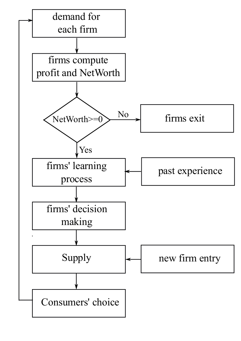
Simulations start with homogeneous firms producing several varieties of the same good. Afterward, firms' decisions and their interactions lead to the emergence of firms' performance differentiation.
Firms' interactions are indirect, deriving essentially from competition for market shares. In fact, in each cycle consumers express their demand, determining firms' profits and their net-worth. Firms with negative net-worth exit from the market, while a new firm enters in both countries each cycle.
According to the learning process, firms that survive take operative decisions regarding the following: investment in productive capacity, research effort, export choice, selling price. Afterward, each firm provides a supply and a new cycle starts.
The model is synthetically described in the following sections, considering the agents (consumers and firms), the stylized assumptions with regard to technological dynamic and the firms' decision process.
Consumers
In the model there are two types of agents: consumers and firms. Consumers have 'ideal variety' preferences, while firms are profit oriented. Consumers and firms are located in two countries; only export firms can sell their product to consumers in both countries, paying an initial fixed cost to enter the foreign market and variable costs of exporting. Consumers and firms are located in cells of two symmetric toroidal spaces (a never ending surface) associated to the two countries. In the toroids the distance between each firm and each consumer represents the difference between consumer's tastes and firm's products characteristics: the shorter the distance, the higher the conformity of the good characteristics to the consumer's preferences. - 2.4
-
Consumers are uniformly distributed in the two toroidal spaces while firms are randomly distributed; at the beginning firms occupy the same positions in the two toroids. Therefore, in the first cycle firm and consumer distributions are identical in the two countries (the two toroids). Firms and consumers can not change their positions, but firms exit from the market when they fail. Moreover when a new firm enters the market its position is assigned randomly. Consequently, the distribution of firms in the two toroids changes in relation to the dynamic of enter and exit of firms.
Firms that choose to export sell their products in the country where they are located (home country or home toroid) and in the other country (the foreign country), while firms that do not export sell only to consumers in the home country.
The position of the good exported in the foreign country is the same position
as the position of the firm in the home country (the two toroids are symmetrical), because each firm produces a specific variety which is the same for the domestic and the foreign countries.
- 2.5
-
Each consumer can buy just one unit of the good produced by the firms. A consumer will not buy any good if there are not enough goods in the market (because of shortage in the supply). Moreover, a consumer does not buy a good if its price is higher than a maximum price (consumer's reserve price) or if the distance between the consumer and the firm that provides the good is too high (consumer's reserve distance). Consumers' preference are ordered according to:
CP = (1/p  )(1/var
 )
)(1)
- 2.6
-
where p is the price of the good and var the square distance between the consumer and the firm that produces the specific good. The coefficients (
 and
and  ) give the relative importance of price and variety in the consumers' preferences and change between consumers. Differences in the distance between firms and consumers gives in aggregate the 'preference for variety' result, which is reinforced by differences in the coefficients of consumers' preferences (in the simulations
 {0.2, 0.5, 0.8}; = 2; 0<var<10; and the reserve price is equal to 17).
Firms
Firms produce a single variety of the market good. They try to increase their profits and, as a simplifying assumption, produce at the maximum of their productive capacity. In the initial cycle all firms have the same characteristics. Production costs are given by a fixed cost (F), plus variable costs measured as unit cost (uc) multiplied by the firm's productive capacity (Cap), plus the unit cost (wa) of research efforts in process innovation multiplied by the amount of investment in research (KA) (in the simulations F=20, wa=1, initial uc=10):C = F + ucCap + waKA (2)
- 2.7
-
Each cycle firms try to sell their product fixing a unit price p; h is the quantity sold that could be equal or less than the quantity produced, in any case costs are computed on the quantity produced. Profit is given by the value of good sold and the production cost (
 =ph - C).
If a firm has a negative net-worth, this firm exits from the market. The net-worth (NW) is given by:
=ph - C).
If a firm has a negative net-worth, this firm exits from the market. The net-worth (NW) is given by:
NW =  +
+  Cap +
Cap +  KA + Mon
(3)
- 2.8
-
where
 ,
,  are, respectively, the productive capacity price and the innovation capital price, Mon is the firm liquidity reserve
(in the simulation ==10, initial liquidity Mon=100, initial productive capacity Cap=10 and initial KA=0).
are, respectively, the productive capacity price and the innovation capital price, Mon is the firm liquidity reserve
(in the simulation ==10, initial liquidity Mon=100, initial productive capacity Cap=10 and initial KA=0).
- 2.9
-
Export firms can not differentiate the product characteristics in the two markets (arbitrage condition):
for each exporter the price and the variety offered are the same in the domestic and in the export markets.
When a firm starts to export it has to pay an initial fixed cost of exporting (Fext). Moreover, exporters pay slightly higher variable costs (iceberg cost
 ) on all the unit of the good they produce (for simplicity if a firm chooses to be an exporter even the units sold on the domestic market are charged by , in simulations =0.05). Therefore, the cost function in the first cycle when a firm enters the foreign market becomes:
C = Fext + F + (uc +  )Cap + waKA
(4)
- 2.10
-
In the following cycles export firms do not have to pay the initial fixed cost of exporting:
C = F + (uc + )Cap + waKA(5)
Technology
Firms are able to make incremental process innovations, which reduce the unit cost (uc). In each cycle, firms choose whether or not to invest in innovation. When firms invest in innovation they pay to buy a single unit of capital needed for innovating (KA=1), for simplicity firms can not accumulate innovative capital.3 Furthermore, firms have to pay the cost (wa) of the workforce employed in research.
The probability to innovate (p(x)) is given by (in the simulations,
to buy a single unit of capital needed for innovating (KA=1), for simplicity firms can not accumulate innovative capital.3 Furthermore, firms have to pay the cost (wa) of the workforce employed in research.
The probability to innovate (p(x)) is given by (in the simulations,  =0.8 and
KA {0, 1}):
=0.8 and
KA {0, 1}):
p(x) =  KA
KA(6)
- 2.11
-
When an innovation occurs the technological capability of the innovating firm (A) increases by one (At=At-1 + 1) and
the associated production cost is given by:
uc = k -  A
A
(7)
- 2.12
-
where k is the starting productivity level, when firms have not introduced any innovation,
and
 an innovation strength parameter (in the simulations k=10 and =0.01).
The Decision Process of Firms
- 2.13
-
In each cycle firms choose:
the selling price, the innovative effort, the size of the productive capacity and whether or not to export.
Firms' choices are independent and are based on a simple reinforcement learning algorithm (Tesfatsion 2005);
in parentheses the value of the parameters used in the simulations).
The results of the different decisions are evaluated according to specific basic
goal functions (according to the profit orientation of firms), which give a real number as response (res).
The probability p(ai) of taking a particular action ai from the set of possible actions is computed using an exponential function to avoid negative values (with 0<
 <1 and 0<ra<1, =0.5 and ra=0.4 for all the choices except for prices where =1.0 to reduce volatility)4:
q(ai)t = (1 - ra)q(ai)t-1 + res(ai)t-1 (8) p(ai) = 
(9)
- 2.14
-
Moreover, each cycle qa(t) is reduced by a small percentage (=0.05) as forgetting and, to allow a continuous exploration of the action space, there is a little probability (
 =0.05) that choices do not depend on past experience.
- 2.15
-
Firms can choose from a limited set of prices (
p {0.5, 1.0, 1.5,...17}): firms can not fix a price that is higher than the consumers' reserve price
(consumers' reserve price is equal to 17) and, given this upper-bound, firms can not set a price that is lower than the marginal cost (no dumping condition).5
- 2.16
-
Firms can increase or decrease their productive capacity (Cap) by only one unit each cycle; furthermore firms
can raise their productive capacity only if they have enough liquidity (
Mon
 , no credit market assumption).
The capital goal function is given by the profit variation which followed the investment choice computed at fixed prices and without fixed cost. In this way, firms may evaluate the effect of a change in the capital stock eliminating price movements and fixed costs; the latter depending on export choices.6
, no credit market assumption).
The capital goal function is given by the profit variation which followed the investment choice computed at fixed prices and without fixed cost. In this way, firms may evaluate the effect of a change in the capital stock eliminating price movements and fixed costs; the latter depending on export choices.6
- 2.17
-
In each cycle, if a firm has enough resources, it may choose whether or not to invest in innovative effort, buying a unit of KA at price and paying a variable cost (wa). The innovative effort is evaluated considering the difference between the productivity improvement effect of the innovative effort (if any) and its cost. 7
- 2.18
-
Firms that enter the foreign market pay an initial fixed sunk cost, therefore:
firms will enter the foreign market only if the difference between expected profits exporting and expected profits just selling domestically are at least equal to or higher than the fixed cost of exporting. However, the learning algorithm is essentially based on past experience, consequently the export choice is modeled in a particular way: when a firm chooses to become an exporter it is forced to stay in the foreign market
for a fixed period of time (as a trial period, e.g. Freund & Pierola,
2010; Eaton et al., 2011). After this period, export firms may be able to compare the profit flows when they export with the ones when they are solely domestic sellers.
In fact, when the trial period ends, export firms will choose whether or not to export: if they choose to continue to export they do not have to pay the fixed cost of exporting; in the next cycle they will choose again. However, if export firms choose to exit the foreign market they become domestic producers; to export again, they have to pay the fixed cost of exporting and they have to enter the trial period.
The trial period might be seen as the consequence of a medium-long run firm's decision as the choice to become an exporter in presence
of fixed cost of exporting (in simulations the trial period is equal to 10 cycles).8Besides, a firm can not become an exporter if it has insufficient liquidity to pay
the initial fixed cost of exporting.
- 2.19
-
Finally, to test the importance of the learning process of firms, simulations in which firms have zero intelligence (Terna 2000) have been run.9
Simulation Results
- 3.1
-
The results of simulations with different cost of exporting are analyzed (Fext is the initial fixed cost of exporting and is the constant variable cost of exporting): Zero Export Costs (ZEC: Fext=0, =0), Medium Export Costs (MEC: Fext=500, =0.05), High Export Costs (HEC: Fext=1000, =0.05).
Simulations with firms that make decisions through the reinforcement learning algorithm (RL) are used to analyze both the ex-ante self-selection and ex-post effects. While to test the importance of the learning process of firms, simulations with zero intelligence firms (ZI) have been run (Terna 2000). Simulation results are analyzed using simple empirical techniques adopted to study export decisions (e.g., Serti & Tomasi 2008, Castellani et al. 2009).
- 3.2
-
From different simulation runs with the same parameters a panel of firms is isolated, comprising all the firms in the last cycles of each simulation, when the number of firms in the market starts to stabilize, conceiving this period as a quasi-equilibrium one.
A panel (just the last 20 cycles of the simulation, 480<cycles<500) is used to have some insights about macro welfare results. While,
to deal with individual firms' characteristics, a longer panel (400 < cycles < 500) is used.
The empirical results are described in the following subsections, which are aimed at dealing with: the better performance of exporters, the ex-ante self-selection effect,
the ex-post effect and some welfare insights.
The Better Performance of Exporters
Simulation data are analyzed implementing pooled and fixed effects regressions, these regressions do not provide any causal explanation, they just attempt to determine whether export firms have a better performance than firms that do not export. Regressions have performance measures as dependent variables: unit cost (the inverse of productivity), production capacity, sales, profit. They have as independent variable a dummy variable that distinguishes between exporters and firms that do not export (Exp). As control (con) there are variables time (cycle) dummies, to avoid system variability and unbalanced panel cohort effects, and dummies for the different simulation runs (Castellani et al. 2009; Bernard et al. 2007a; Serti & Tomasi 2008).10 - 3.3
-
The fixed effects regressions, eliminating every constant individual characteristic, consider only the firms that change their openness status: they become exporter or they leave the export market. Therefore, in fixed effects regressions the export dummy parameters might be interpreted as an approximate measure of performance improvements of the firms that become exporters. In the case of pooled regressions and fixed effects regressions respectively:
yit =  +
+  Expit +
  conit + eit
(14) yit = + Expit + conit +  + eit
+ eit(15)
Table 1: ZI, Exporter Premia: (Pooled (pr) and fixed effects (fe) regressions) ZEC(pr) ZEC(fe) MEC(pr) MEC(fe) HEC(pr) HEC(fe) Unit cost 0.01** 0.001 -0.27** 0.001 -0.29** 0.001 (0.001) (0.001) (0.005) (0.001) (0.005) (0.001) Prod. Cap -0.06** -0.001 9.94** 0.76** 17.61** 1.17** (0.014) (0.005) (0.093) (0.017) (0.149) (0.027) Sales 0.29** 0.35** 10.19** 0.95** 17.88** 1.26** (0.017) (0.011) (0.092) (0.019) (0.149) (0.029) Profit 4.75** 5.08** -12.87** -56.16** -46.61** -124.92** (0.195) (0.184) (0.474) (0.230) (0.809) (0.438) n. firms 12,860 12,910 12,970 Note: Standard error in parentheses below the coefficients. Asterisks denote significance levels (**: p < 5%; *: p < 10%). Regressions include time (cycle) and simulation run dummies.
- 3.4
-
In simulations with zero intelligence firms (ZI), pooled regressions (table 1) show that with cost of exporting (MEC and HEC) export firms present: lower unit costs (higher productivity), higher productive capacity, higher sales, but lower profit. Meanwhile, in zero export cost simulations (ZEC), exporters have slightly lower productivity and lower productive capacity, but higher profits. In all the regressions the coefficients of sales are positive and significant: sales are higher for exporters because market opportunities rise when firms export. Therefore, the high productive capacity is likely to increase the survival possibilities of export firms compensating for export costs.
- 3.5
-
In fixed effects regressions, which could give some insight into the consequences of the choice to export, there is no significant relationship between exporting and productivity (unit cost). Thus, with zero intelligence exporting might not result in any significant improvement in productivity. Consequently, with costs of exporting, the lower level of unit cost registered in pooled regressions may be
just the result of the ex-ante self-selection effect: firms with low unit cost (high productivity) could make high profit and accumulate large liquidity, allowing them to pay the initial fixed cost of exporting needed to enter the foreign market.
Note: Standard error in parentheses below the coefficients. Asterisks denote significance levels (**: p < 5%; *: p < 10%). All regressions include time (cycle) and simulation run dummies.Table 2: RL, Exporter Premia, (Pooled (pr) and fixed effects (fe) regressions) ZEC(pr) ZEC(fe) MEC(pr) MEC(fe) HEC(pr) HEC(fe) Unit cost 0.04** 0.01** -0.66** -0.01** -0.67** -0.01** (0.009) (0.001) (0.011) (0.001) (0.010) (0.001) Prod. Cap. 13.23** 2.32** 24.97** 4.23** 28.47** 6.58** (0.321) (0.104) (0.356) (0.116) (0.355) (0.136) Sales 15.52** 6.53** 25.84** 7.50** 28.72** 9.68** (0.334) (0.130) (0.351) (0.129) (0.338) (0.139) Profit 129.83** 81.98** 198.73** 39.29** 202.96** 22.58** (2.872) (1.510) (3.052) (1.582) (3.106) (1.818) n. firms 9,598 10,951 12,378
- 3.6
-
Data from simulations (table 2) with costs of exporting and reinforcement learning (RL) show the better performance of exporters in all the dimensions taken into consideration, in accordance with the empirical evidence.
- 3.7
-
Profit is higher for exporters in reinforcement learning simulations (RL) than in ZI ones. In fact, in zero intelligence simulations (ZI),
firms choose randomly to become or to remain exporters; therefore, even if exporting lead to higher profits, export firms might choose (randomly) to exit from the foreign market.
- 3.8
-
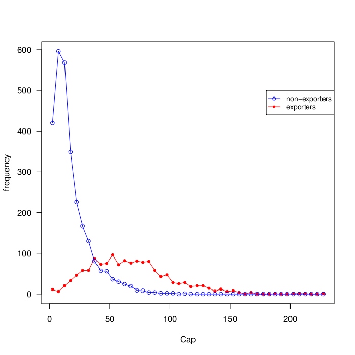
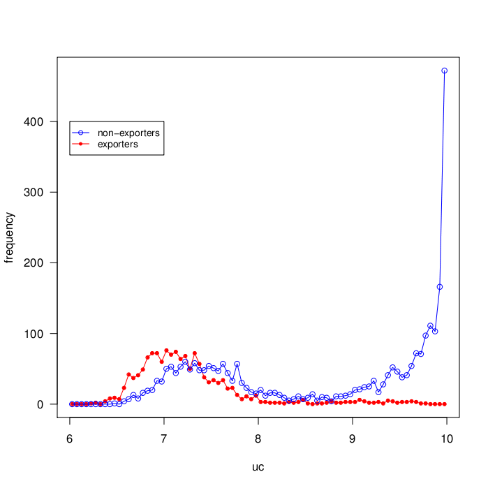
In reinforcement learning simulations (RL), the relative performance of export firms is better in the high export cost simulations (HEC). 11 With zero export costs (ZEC) sales, profit and the productive capacity rise when a firm exports because entering the foreign market increases firms' selling opportunities. However, in ZEC the unit cost of exporters is slightly higher, while in HEC and MEC the unit cost of exporters is considerably lower. In fact, the fixed cost of exporting represents an obstacle to exploiting
foreign market opportunities, which only firms that are large or have high productivity can overcome (ex-ante self-selection effect). Moreover, considering fixed effects regressions, simulations with costs of exporting show lower unit cost for exporters: becoming an exporter
may lead to productivity growth. Therefore, in simulations with reinforcement learning and costs of exporting (MEC, HEC) the ex-post effect may also emerge as a determinant of the better performance of exporters.
(The distribution of the size of the firms in terms of productive capacity
and the distribution of unit costs in MEC simulations are reported
in figure 2 and 3 respectively)
- 3.9
-
Considering MEC simulations with reinforcement learning and examining micro properties to illustrate market results,
it is possible to run regressions to test the relationships between firm characteristics (Unit cost: uc; price: p; profit and productive capacity: Cap) and dummies for exporting (Exp). As controls (con) there are time (cycle) and run dummies. Implementing pooled and fixed effects regressions:
yit = + Expit + Capit +  pit +
pit +  conit + eit
(16) yit = + Expit + Capit + pit + conit + + eit(17)
Note: Standard error in parentheses below the coefficients. Asterisks denote significance levels (**: p < 5%; *: p < 10%). All regressions include time (cycles) and simulation run dummies, R2 of fixed effects regressions are just the R2 of transformed data regressions.Table 3: Micro Properties (Pooled (pr) and fixed effects (fe) regressions) uc(pr) uc(fe) p(pr) p(fe) profit(pr) profit(fe) Exp -0.411** -0.004** 0.338** 0.241** 3.270** 4.454** (0.0088) (0.0004) (0.0109) (0.0072) (1.4357) (1.3691) Prod. Cap. -0.010** -0.001** -0.016** -0.012** 6.833** 6.865** (0.0001) (0.0001) (0.0003) (0.0003) (0.0579) (0.0523) Unit cost -0.676** 1.478** -17.568** -58.491** (0.0112) (0.0880) (0.6384) (7.6027) Price 33.918** 29.953** (0.3959) (0.3828) R2 0.22 0.93 0.18 0.03 0.72 0.33 firms 10,951
- 3.10
-
The lower unit cost for exporters is evident even when controlling for the productive capacity (table 3).
Additionally, exporters could fix higher prices, because they have a larger selling market. Both lower unit costs and higher prices, considering also the higher productive capacity (table 2), lead to higher profits for exporters.
Ex-ante Self-Selection Effect
- 3.11
-
In order to deal with the dynamic of different firm performance dimensions in relation to export decisions, a subset of firms
in reinforcement learning simulations is isolated: this subset is composed of firms that start to export during the panel time span and the never exporting firms are used as control group.
A simple regression is used to evaluate ex-ante differences in t - periods before entering, with a dummy variable which distinguishes between entering and non-entering firms to foreign market (Ent) in the cycle t,
and controls (con) of simulation runs and time (cycles) (Castellani et al. 2009; Serti & Tomasi 2008; Bernard et al. 2007a):
yi(t-  ) = + Enti + conit + eit
(18)
Note: Standard error in parentheses below the coefficients. Asterisks denote significance levels (**: p < 5%; *: p < 10%). All regressions include time (cycle) and simulation run dummies.Table 4: RL MEC, Ex-Ante Performance (Pooled regressions) Unit Cost Prod. Cap. Sales Profit t-25 -1.86** 18.5** 17.1** 155.8** (0.053) (1.367) (1.248) (10.70) t-20 -1.86** 18.3** 17.1** 172.5** (0.053) (1.298) (1.203) (9.88) t-15 -1.87** 17.5** 15.9** 176.4** (0.053) (1.243) (1.148) (9.67) t-10 -1.88** 17.6** 16.6** 189.7** (0.053) (1.235) (1.129) ( 9.20) t-5 -1.88** 18.3** 16.4** 184.7** (0.053) (1.238) (1.075) (8.77) t -1.89** 19.8 18.6** -272.7** (0.053) (1.249) (1.219) (11.02)
- 3.12
-
Considering only the MEC simulations (table 4), the coefficients confirm the presence of the ex-ante self-selection effect. The ex-ante effect is reinforced when the entering lag is reduced, while in time (cycle) t there is a significant profit decrease
for entering firms because they have to sustain the initial fixed cost of exporting.
Looking at the other simulation specifications (table 5), there is no ex-ante self-selection with zero cost of exporting (ZEC). Self-selection is higher in simulations with high costs of exporting (HEC): the higher the obstacle to enter the foreign market, the higher
the pre-entering productivity needed to overcome it.
Note: Standard error in parentheses below the coefficients. Asterisks denote significance levels (**: p < 5%; *: p < 10%). All regressions include time (cycle) and simulation run dummies.Table 5: Ex-ante Unit Costs, (Pooled regressions) Zero EC Medium EC High EC t-25 -0.06 -1.86** -2.13** (0.836) (0.053) (0.035) t-20 -0.06 -1.86** -2.13** (0.845) (0.053) (0.035) t-15 -0.06 -1.87** -2.14** (0.853) (0.053) (0.035) t-10 -0.07 -1.88** -2.15** (0.858) (0.053) (0.035) t-5 -0.07 -1.88** -2.15** (0.862) (0.053) (0.035) t -0.07 -1.89** -2.16** (0.866) (0.053) (0.035)
Ex-Post Effect
- 3.13
-
To test the importance of the ex-post effect, fixed effects regressions have been implemented, controlling for invariable firms' characteristics. These regressions have as dependent variable the performance measures. As independent variables dummies (Dkit) refer to pre-entering periods if k is negative and post-entering periods if k is positive, Dkit dummies are equal to one if firms enter the foreign market in the period t. As controls, there are time (cycle) dummies (Serti & Tomasi 2008; Jacobson et al. 1993).
In this way, it is in part possible to isolate the dynamic of productivity (inverse of the unit cost) for entrants from the overall sample, controlling also
for idiosyncratic characteristics of firms.
yit = +  Dkit + cont + + eit
(19)
Note: Standard error in parentheses below the coefficients. Asterisks denote significance levels (**: p < 5%; *: p < 10%). All regressions include time (cycle) and simulation run dummies.Table 6: Ex-ante and Ex-Post Performance, (fixed effects regressions) Unit Cost Prod. Cap. Sales Profit t-25 -0.001** 0.35** 0.11 0.8 (0.0003) (0.051) (0.240) (3.57) t-20 -0.006** 2.13** 2.47** 21.7** (0.0012) (0.300) (0.390) (5.27) t-10 -0.024** 6.28** 6.47** 52.3** (0.0024) (0.609) (0.589) (5.96) t-1 -0.042** 9.59** 2.84** -69.0** (0.0034) (0.802) (1.040) (13.94) t -0.044** 9.98** 9.99** -404.6** (0.0035) (0.811) (0.849) (10.06) t+10 -0.065** 14.39** 15.75** 135.5** (0.0044) (0.972) (0.909) (10.24) t+20 -0.089** 18.65** 20.00** 171.8** (0.0050) (1.249) (1.160) (10.99) t+25 -0.101** 20.31** 21.46** 185.35** (0.0053) (1.317) (1.317) (12.45)
- 3.14
-
In MEC simulations (table 6), regressions show that, in all the dimensions, the exporter premia tends to increase over time (cycle).
Profit is relatively reduced in the year before entering the foreign market, because it is likely that
a firm chooses to change its selling strategy, becoming an exporter, as a reaction to a negative shock which led to negative profit. Negative shocks
are the result of firms interactions; for instance, a firm might be hit by a negative shock if its market share is reduced because competitors that have
invested in research are able to reduce unit costs and, thus, prices.
Moreover, in the first cycle after entering the foreign market, profits are severely reduced by the fixed cost of exporting. Considering the zero cost of exporting specification (ZEC), unit costs are higher but
after entering they are not significant, while unit costs are lower for entrant firms in MEC and HEC (table 7).
Note: Standard error in parentheses below the coefficients. Asterisks denote significance levels (**: p < 5%; *: p < 10%). All regressions include time (cycle) and simulation run dummies.Table 7: Ex-Ante and Ex-Post Unit Costs (fixed effects regressions) Zero EC Medium EC High EC t-25 -0.001 -0.001** -0.001** (0.0010) (0.0003) (0.0003) t-20 0.003* -0.006** -0.006** (0.0019) (0.0012) (0.0010) t-10 0.010** -0.024** -0.018** (0.0042) (0.0024) (0.0022) t-1 0.013** -0.042** -0.034** (0.0065) (0.0034) (0.0028) t 0.013** -0.044** -0.036** (0.0065) (0.0035) (0.0029) t+10 0.016* -0.065** -0.056** (0.0088) (0.0044) (0.0034) t+20 0.015 -0.089** -0.077** (0.0106) (0.0050) (0.0038) t+25 0.013 -0.101** -0.089** (0.0115) (0.0053) (0.0040)
- 3.15
-
To have some insight into the unit cost dynamic it is also possible to consider the unit cost growth rates using a simple regression:
yi(t- )/yi(t--k) = + Enti + conit + eit(20)
Note: Standard error in parentheses below the coefficients. Asterisks denote significance levels (**: p < 5%; *: p < 10%). All regressions include time (cycle) and simulation run dummies.Table 8: Growth Rates of Unit Costs (Pooled regressions) Zero EC Medium EC High EC (t-20)/t-25) 0.0009 -0.0013** -0.0015** (0.0016) (0.0001) (0.0001) (t-15)/(t-20) -0.0006 -0.0017** -0.0016** (0.0016) (0.0001) (0.0001) (t-10)/(t-15) -0.0009 -0.0013** -0.0014** (0.0013) (0.0001) (0.0001) (t-5)/(t-10) -0.0001 -0.0013** -0.0014** (0.0012) (0.0001) (0.0001) t/(t-5) -0.0002 -0.0015** -0.0015** (0.0009) (0.0001) (0.0001) (t+5)/t 0.0003 -0.0016** -0.0015** (0.0007) (0.0001) (0.0001) (t+10)/(t+5) 0.0003 -0.0018** -0.0018** (0.0009) (0.0001) (0.0001) (t+15)/(t+10) -0.0018** -0.0020** -0.0019** (0.0009) (0.0001) (0.0001) (t+20)/(t+15) -0.0007 -0.0020** -0.0017** (0.0005) (0.0001) (0.0001) (t+25)/(t+20) 0.0009 -0.0022** -0.0021** (0.0008) (0.0001) (0.0001)
- 3.16
-
In MEC and HEC, the firms' growth rates of productivity accelerate after entering the foreign market, while growth
rates are not significant in ZEC (table 8).
- 3.17
-
The ex-post effect emerges in simulations with firms' reinforcement learning
solely as a consequence of the initial fixed cost of exporting. In fact, without any assumptions about increasing technological spillovers for exporters, the ex-post effect may be interpreted as a dynamic consequence of the self-selection effect caused by fixed cost of exporting: firms that have good performance (high productivity, high sales) are able to overcome the fixed cost of exporting, as these firms have taken good competitive decisions in their past and, through reinforcement learning, they will make good decisions in future. Moreover, when firms start exporting they can exploit larger market opportunities, which augment their capacity to sustain innovative efforts. Therefore, assuming that, at least in part firms make decisions following reinforcement learning mechanisms, it seems possible that, to some extent, the post-entry effect shown by empirical researches may be the result of a virtuous learning process derived from the initial fixed cost of exporting, combined with greater selling opportunities.
Welfare Insights
- 3.18
-
To have some insight into the effects of export costs on welfare, the data from simulations of the three export cost specifications (ZEC, MEC, HEC) with reinforcement learning (RL) are merged, averaging the last 20 cycles' values for all firms. This dataset is analyzed implementing regressions with unit cost, price and profit as dependent variables. As independent variables dummies for the export cost specifications (medium cost DM, high cost DH and zero cost of exporting DZ) are used. As control variables (con) there are firms characteristics interacting with the export cost specifications dummies: the productive capacity (CapZ, CapM, CapH), exporter dummy (ExpZ, ExpM, ExpH) and unit cost (UcZ, UcM, UcH).12
Interactions with the dummies of the export cost specifications are necessary because data coming from different simulation specifications are merged,
leading to structural breaks.
yi = + MECi + HECi + coni + ei(21)
Note: Standard error in parentheses below the coefficients. Asterisks denote significance levels (**: p < 5%; *: p < 10%). Coefficients and standard errors are rounded.Table 9: Welfare Insights, (OLS regressions) Unit cost Price Profit DM 0.52** 2.03** -95.97** (0.037) (0.159) (11.838) DH 0.27** 2.34** -148.09** (0.035) (0.162) (11.069) CapZ -0.017** -0.015** 6.00** (0.0003) (0.0005) (0.078) CapM -0.008** -0.016** 6.60** (0.0003) (0.0004) (0.087) CapH -0.005** -0.016** 6.21** (0.0003) (0.0004) (0.095) ExpZ 0.52** -0.017** 25.50** (0.041) (0.051) (3.705) ExpM -1.15** 0.48** 28.82** (0.032) (0.037) (3.929) ExpH -1.09** 0.69** 52.71** (0.025) (0.036) (4.403) UcZ -0.39** 6.00** (0.015) (0.0780) UcM -0.58** 6.60** (0.012) (0.0873) UcH -0.63** 6.21** (0.013) (0.095) R2 0.28 0.30 0.87 n. firms 25.297
- 3.19
-
Without costs of exporting the market environment is more competitive, thus at the end of the simulations the number of firms operating is
lower with respect to medium and high cost specifications (the average number of firms in ZEC is 369, in MEC: 420.6, in HEC: 475.35), but at the same time the smaller number of firms is compensated by a higher share of export firms (the average share of export firms in ZEC: 0.64, in MEC: 0.42, in HEC: 0.32).
In the zero cost of exporting environment controlling for firms characteristics, on average firms reach higher productivity (lower unit cost), lower prices and also higher profit. Therefore, in the zero cost of exporting specification tougher competition might lead to higher welfare for consumers, thanks to more varieties available due to the higher number of exporters and thanks to lower unit costs and lower prices controlling for firms characteristics.
Conclusions
- 4.1
-
This agent based model is, in part, an attempt to analyze the better performance of exporters deriving firm heterogeneity as the emergent result of
firms' choices and interactions. The model is limited by the simplicity of the firms' decision- making algorithm, which is based on a basic reinforcement learning algorithm (Tesfatsion 2005; Roth & Erev 1993). Moreover, the model's parametric space is large and only the most important parameters have been explored. Besides, several structural changes can be implemented, for instance modifying starting conditions, temporal and spatial dimensions, technological development characteristics, arbitrage conditions, etc...
- 4.2
-
On the other hand, the agent based
model presents some advantages: the possibility to model bounded rationality in firm choices, conceiving firm heterogeneity as an emerging result of endogenous technological change, dealing with dynamic and path dependent processes. Moreover, the simplicity of the firms decision-making algorithm could be seen as a benchmark, giving robust results and transparency to individual firms' choice processes.
- 4.3
-
The simulation model is able to replicate the better performance of export firms, reproducing both the ex-ante self-selection and the ex-post effects. In the agent based model, the firm productivity distribution is endogenous, being the result of firms' choices determined by learning processes. Consequently, in the simulations the export premia emerges because firms that have better performance are able to overcome the fixed cost of exporting (the self-selection effect) and export firms increase their performance with respect to non-exporters (ex-post effect). The ex-post effect is the result of the increasing market opportunities for the exporter and, at the same time, the consequence of the dynamic characteristics of the learning process: firms that are able to overcome the initial fixed cost of exporting are those firms that have made good choices in their past and are likely to continue to make good choices in their future.
- 4.4
-
If the ex-post effect derives from increasing knowledge spill-over for exporters, encouraging firms to export could result in increasing aggregate efficiency.
However, simulations reproduce the ex-post effect without assuming the presence of any knowledge spillover, thus the model empathizes the importance of firms' learning processes and costs of exporting in determining the ex-post improvement effect. For these reasons, greater attention might be given to the incentives that lead firms to make virtuous reinforcing competitive choices which allow them to enter foreign markets. Moreover, according to the simulation results, at aggregate level, reducing the cost of exporting raises competition, which leads to higher levels of productivity and lower prices,
improving consumers' welfare.
- 4.5
-
Finally, this model could be adapted to study other connected international trade topics, for instance the aggregate welfare effects of changes in costs of exporting in the case of non-homogeneous countries with differences in technological capabilities or endowments. It could also be possible to enlarge the model to deal with international production fragmentation and, therefore, sourcing and foreign investment choices.
Notes
- 1
- Some empirical research: Clerides et al. (1998); Bernard & Jensen (1999); Castellani et al. (2009); Serti & Tomasi (2008); Alvarez & Lopez (2005); Aw et al. (2000).
- 2
- Some of the models that follow the Melitz (2003) approach are: Helpman et al. (2008); Bernard et al. (2007b); Helpman et al. (2004); Antras & Helpman (2004). The Melitz & Ottaviano (2008) model does not assume the presence of fixed costs of exporting and is based on a quasi-linear utility function for the representative consumer. An alternative approach is Bernard et al. (2003), which assumes Bertrand competition.
- 3
- Each cycle after the innovative research is accomplished, whether or not it leads at an innovation, the innovative capital KA is sold at price . This simplification is useful, from one side, to treat KA and Cap as similar entities and, from the other side, for firms to easily understand the real benefit of the innovative effort, which otherwise could be obscured by the accumulation of KA. In any case, specifications of the model with the possibility of accumulating KA do not lead to structurally different results in terms of differences between exporters and not exporters.
- 4
- It is important to reduce price choice volatility, because firms may have to choose among a relatively high number of prices and prices have strong effects on firms'results.
- 5
-
The goal function of price setting is given by:
res(t-1) = p(t-1)(1 - 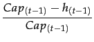 )
)(10)
where p(t-1) is the price chosen in t-1. Cap(t-1) is the productive capacity and h(t-1) is the number of goods sold ( h(t-1) Cap(t-1)). Thus, res is given by the returns weighted by sales on total productive capacity, because increasing prices, from one hand, has the effect of rising
returns on each good but, from the other hand, might reduce the total amount of goods sold.
Cap(t-1)). Thus, res is given by the returns weighted by sales on total productive capacity, because increasing prices, from one hand, has the effect of rising
returns on each good but, from the other hand, might reduce the total amount of goods sold.
- 6
- The goal function for capital investment is given by differences in net revenues NR, conceived as profit at fixed prices without fixed costs:
res(t-1) = NR(t-1) - NR(t-2) (11)
- 7
- The goal function of the investment in research choice is given by:
res(t-1) =  (-
(-  uc(t-1))Cap(t-1) - waKA/
(12)
( - uc(t-1)) is the productivity improvement effect and
waKA/
uc(t-1)) is the productivity improvement effect and
waKA/ is the relative cost of the innovative effort.
(
is the relative cost of the innovative effort.
( =10 and =125, the value of and parameters are chosen to let the expected value of the innovative choice to be positive
in the first cycle, assuming for learning purposes that at the beginning of the simulations innovating might be seen as a good choice for firms).
=10 and =125, the value of and parameters are chosen to let the expected value of the innovative choice to be positive
in the first cycle, assuming for learning purposes that at the beginning of the simulations innovating might be seen as a good choice for firms).
- 8
- The export goal function is given by profit:
res(t-1) = 
(13)
- 9
- Simulations have been run with different knowledge parameters in particular considering different levels of the learning parameter (ra) , they produce results that are not sensibly different from the ones deriving from the parameters used in the model except when ra=1 or ra=0.
- 10
- Regressions with unit cost as dependent variable, using productive capacity as control, have also been run but they do not lead to significant differences. Controlling for the productive capacity may be necessary in the hypothesis that productivity depends on the production scale, but it is not the case in this model.
- 11
- To have an idea of the coefficient dimensions, the unit cost level varies between 1 and 10.
- 12
- The productive capacity dummies: CapZ= Cap . DZ, CapM= Cap . DM, CapH= Cap . DH, the exporter dummies: ExpZ= Exp . DZ, ExpM= Exp . DM, ExpH= Exp . DH, and unit cost dummies: UcZ= Uc . DZ, UcM= Uc . DM, UcH= Uc . DH.
References
-
ACEMOGLU, D. (2009).
Introduction to Modern Economic Growth.
Princeton University Press.
ALVAREZ, R. & LOPEZ, R. (2005). Exporting and performance: Evidence from Chilean plant. Canadian Journal of Economics 4(38). [doi:10.1111/j.0008-4085.2005.00329.x]
ANTRAS, P. & HELPMAN, E. (2004). Global sourcing. Journal of Political Economy 112(3). [doi:10.1086/383099]
ARTHUR, B. W., DURLAUF, S. & LANE, D. (1997). Introduction: Process and emergence in the economy. In: The Economy as an Evolving Complex System II (ARTHUR, B. W., DURLAUF, S. & LANE, D., eds.). Addison-Wesley. [doi:10.1017/cbo9781139174596.003]
AW, B. Y., CHUNG, S. & ROBERTS, M. J. (2000). Productivity and turnover in the export market: Micro-level evidence from the Republic of Korea and Taiwan (China). World Bank Economic Review 14(1). [doi:10.1093/wber/14.1.65]
BERNARD, A. B., EATON, J., JENSEN, J. B. & KORTUM, S. (2003). Plants and productivity in international trade. American Economic Review 39(4). [doi:10.1257/000282803769206296]
BERNARD, A. B., JENSEN, B. J., REDDING, S. J. & SCHOTT, P. K. (2007a). Firms in international trade. Journal of Economic Perspectives 21(3). [doi:10.1257/jep.21.3.105]
BERNARD, A. B., JENSEN, B. J. & SCHOTT, P. K. (2007b). Comparative advantage and heterogeneous firms. Review of Economic Studies 74(1). [doi:10.1111/j.1467-937X.2007.00413.x]
BERNARD, A. B. & JENSEN, J. B. (1999). Exceptional exporter performance: cause, effect, or both? Journal of International Economics 47(1). [doi:10.1016/S0022-1996(98)00027-0]
BERNARD, A. B. & JENSEN, J. B. (2004). Why some firms export. The Review of Economics and Statistics 86(2). [doi:10.1162/003465304323031111]
BERNARD, J., JENSEN, J. B. & SCHOTT, P. (2005). Importers, exporters, and multinationals: A portrait of firms in the U.S. that trade goods. Center for Economic Studies, U.S. Census Bureau (05-20).
BURSTEIN, A. & MELITZ, M. J. (2011). Trade liberalization and firm dynamics. NBER Working Papers 16960, National Bureau of Economic Research, Inc.
BUSTOS, P. (2011). Trade liberalization, exports, and technology upgrading: Evidence on the impact of Mercosur on Argentinian firms. American Economic Review 101(1), 304–40. [doi:10.1257/aer.101.1.304]
CASTELLANI, D., SERTI, F. & TOMASI, C. (2009). Firms in international trade: Importers and exporters heterogeneity in the Italian manufacturing industry. The World Economy (33).
CLERIDES, S., LACH, S. & TYBOUT, J. (1998). Is learning by exporting important? Micro-dynamic evidence from Colombia, Mexico, and Morocco. Quarterly Journal of Economic 113(3). [doi:10.1162/003355398555784]
COSTANTINI, J. & MELITZ, M. J. (2007). The dynamics of firm-level adjustment to trade liberalization. In: The Organization of Firms in a Global Economy (HELPMAN, E., MARIN, D. & VERDIER, T., eds.). Cambridge: Harvard University Press.
EATON, J., Eslava, M., Krizan, C. J., Kugler, M. & Tybout, J. (2011). A search and learning model of export dynamics. Mimeo, Pennsylvania State University.
FEENSTRA, C. R. (2003). Advanced International Trade: Theory and Evidence. Princeton University Press.
FREUND, C. & Pierola, M. D. (2010). Export entrepreneurs : evidence from Peru. Policy Research Working Paper Series 5407, The World Bank. [doi:10.1596/1813-9450-5407]
GILBERT, N. & TERNA, P. (2000). How to build and use agent-based models in social science. Mind & Society: Cognitive Studies in Economics and Social Sciences 1(1).
HELPMAN, E. H., MELITZ, M. J. & RUBINSTEIN, Y. (2008). Estimating trade flows: Trading partners and trading volumes. Quarterly Journal of Economics 123(2). [doi:10.1162/qjec.2008.123.2.441]
HELPMAN, E. H., MELITZ, M. J. & YEAPLE, S. R. (2004). Export. versus FDI with heterogeneous firms. American Economic Review. 1(94). [doi:10.1257/000282804322970814]
JACOBSON, L., LALONDE, R. & SULLINVAN, D. (1993). Earnings losses of displaced workers. American Economic Review 4(8).
KIRMAN, A. (2011). Learning in agent based models. Eastern Economic Journal 37(1). [doi:10.1057/eej.2010.60]
MANASSE, P. & TURRINI, A. (2001). Trade, wages, and 'superstars'. Journal of International Economics 54(1), 97-117. [doi:10.1016/S0022-1996(00)00090-8]
MELITZ, M. J. (2003). The impact of trade on intra-industry reallocations and aggregate industry productivity. Econometrica 6(71). [doi:10.1111/1468-0262.00467]
MELITZ, M. J. & OTTAVIANO, G. (2008). Market size, trade, and productivity. Review of Economic Studies 75(1). [doi:10.1111/j.1467-937X.2007.00463.x]
ROBERTS, M. J. & TYBOUT, J. R. (1997). The decision to export in colombia: An empirical model of entry with sunk costs. The American Economic Review 87(4).
ROTH, A. E. & EREV, I. (1993). Learning in extensive form games: experimental data and simple dynamic models in the intermediate term. Games and Economic Behaviour (8).
SERTI, F. & TOMASI, C. (2008). Self selection and post-entry effects of exports. evidence from Italian manufacturing firms. Review of World Economics 4(144). [doi:10.1007/s10290-008-0165-9]
SIMON, H. A. (1979). Rational decision making in business organizations. American Economic Review 69(4).
TERNA, P. (2000). The "mind or no mind" dilemma in agents behaving in a market. In: Applications of Simulation to Social Sciences (BALLOT, G. & WEISBUCH, G., eds.). Hermes Science. [doi:10.1142/s0219525900000194]
TERNA, P. (2011). Slapp-python protocol. http://eco83.econ.unito.it/terna/slapp/.
TESFATSION, L. (2005). Agent-based computational economics: a constructive approach to economic theory. In: Handbook of Computational Economics 2 (TESTFATSION, L. & JUDD, K. L., eds.). North-Holland.
YEAPLE, S. R. (2005). A simple model of firm heterogeneity, international trade, and wages. Journal of International Economics 65(1). [doi:10.1016/j.jinteco.2004.01.001]