
 Abstract
- This paper illustrates the use of the nonparametric Wald-Wolfowitz test to detect stationarity and ergodicity in agent-based models. A nonparametric test is needed due to the practical impossibility to understand how the random component influences the emergent properties of the model in many agent-based models. Nonparametric tests on real data often lack power and this problem is addressed by applying the Wald-Wolfowitz test to the simulated data. The performance of the tests is evaluated using Monte Carlo simulations of a stochastic process with known properties. It is shown that with appropriate settings the tests can detect non-stationarity and non-ergodicity. Knowing whether a model is ergodic and stationary is essential in order to understand its behavior and the real system it is intended to represent; quantitative analysis of the artificial data helps to acquire such knowledge.
- Keywords:
- Statistical Test, Stationarity, Ergodicity, Agent-Based, Simulations
Introduction
- 1.1
- The aim of this paper is to present a set of nonparametric tools to perform a quantitative analysis of the emergent properties of an agent-based model, in particular to assess stationarity and ergodicity. Modeling a system by using an agent-based model implies assuming that no explicit mathematical form can explain the behavior of the system. The impossibility of having an analytical form of the data generator process and the difficulty in understanding how the random component influences the process, require—besides the traditional parametric tools—nonparametric statistics and tests. The choice of a nonparametric test instead of the traditional parametric tests derives from the particular problem faced. As stated by Siegel (1957, p. 14): "By a criterion of generality, the nonparametric tests are preferable to the parametric. By the single criterion of power, however, the parametric tests are superior, precisely for the strength of their assumptions". Any conclusion derived from using parametric tests is valid only if the underlying assumptions are valid. Since the objective is to analyze the behavior of the model, the test can be performed on the artificial data. By construction the stochastic behavior of the model is unknown, while the power problem of nonparametric tests can easily be solved by increasing the number of observations; in that way nonparametric tests are perfectly suited for testing agent-based models. By considering the agent-based model as a good approximation of the real data generator process, the tests on artificial data can also be used to make inferences on the real data generator process.
- 1.2
- Knowledge of the basic properties of the artificial time series is essential to reach a correct interpretation of the information which can be extracted from the model. To acquire such knowledge it is important to perform statistical testing of the properties of the artificial data (Leombruni and Richiardi 2005; Richiardi et al. 2006). Supposing that an agent-based model has a statistical equilibrium, defined as a state where some relevant statistics of the system are stationary (Richiardi et al. 2006) the stationarity test can help in detecting it. The ergodicity test helps in understanding whether the statistical equilibrium is unique (conditional to the parameters of the model) regardless of the initial conditions. Whether the aim is to compare the moments of the agent-based model with different parameter settings with observed data or to estimate the structural parameters, it is necessary to know if the model produces stationary and ergodic series. If the artificial data are stationary and ergodic, a different emphasis can be given to the theoretical and empirical results of the model and artificial and real data can be compared to estimate the structural parameters (Gilli and Winker 2003; Grazzini 2011a). One aim of the paper is to underline the importance of statistical tests for stationarity and ergodicity as complementary tools in addition to sensitivity analysis and other quantitative studies over the behavior of the agent-based model to have a deeper understanding of the model itself. Another aim of the paper is to describe nonparametric tests for stationarity and ergodicity easy to use and to apply to agent-based models. The stationarity test is described in section 2 and the ergodicity test is described in section 3. Performance of the tests has been evaluated using the Monte Carlo method[1] and applied to a simple agent-based model in section 4.
Stationarity
- 2.1
- Stationarity is the property of a process necessary to estimate consistently the moments using the observations of the time series. The properties of a strictly stationary data generator process are constant in time. This implies that each observation can be considered as an extraction from the same probability distribution and that each observation carries information about the constant properties of the observed realization of the data generator process[2]. In agent-based models the stationarity test is important to know whether the model reaches a statistical equilibrium state. Given a stochastic process {Xt} t=1,2,…., {Xt} is strictly stationary if Xt has the same distribution for every t, and the joint distribution of (Xt,Xt1,Xt2,…,Xtn) depends only on t1-t,t2-t,… and not on t. A less demanding definition of stationarity is the covariance stationarity. A stochastic process is covariance stationary if E(Xt)=μ is independent of t, and if the covariance Cov(Xt,Xt-j) depends only on j. An example of a strictly stationary process is the white noise, with xt=ut where ut is i.i.d. Examples of non-stationary series are the returns in a stock market, where there is clustered volatility (the variance changes during the series) and GDP time series exhibiting time trends like most aggregate time series (Hayashi 2000).
- 2.2
- Stationarity is a very important property of time series since it has both theoretical and practical implications. For this reason there is a wide variety of tests to verify the stationarity of time series (see Phillips and Xiao 1998 for a survey). Dickey-Fuller tests (Dickey and Fuller 1979; 1981) are unit root tests (the null-hypothesis is nonstationarity) based on an autoregressive process of known order with independent and identical distributed (iid) errors, ut. The test needs quite strong hypotheses: the knowledge of the model producing the time series and the assumptions on the error term. An important extension of the test was proposed by Said and Dickey (1984) where it is shown that the original Dickey-Fuller procedure is valid also for a more general ARIMA(p,1, q) in which p and q are unknown. The extension allows using the test in the presence of a serial correlated error term. Adding lags to the autocorrelation allows the elimination of the effect of serial correlation on the test statistics (Phillips and Xiao 1998). An alternative procedure was proposed by Phillips (1987) using a semi-parametric test (Phillips and Xiao 1998) allowing the error term to be weakly dependent and heterogeneously distributed (Phillips 1987; Phillips and Perron 1988). Another test proposed as complementary to the unit root tests is the KPSS test (Kwiatkowski, Phillips, Schmidt and Shin 1991) in which the null-hypothesis instead of being nonstationarity is stationarity. Note that all the tests described above are parametric in the sense that they need assumptions about the stochastic process generating the tested time series. In a framework where the complexity of the model is such that an analytical form has been regarded as not able to represent the system, such assumptions over the data generator process may be too restrictive. Therefore, in addition to the parametric tests, it can be interesting to perform a nonparametric test that does not need any assumption over the data generator process. As noted in the introduction, the problem with parametric tests is the power of the test. Fewer assumptions imply the need for more information thus more observations. Given that the test will be made on the artificial data, the power of the test is not a problem since the number of available observations can be increased at will with virtually no costs. Our interest is to understand how a given set of moments of the simulated time series behaves. If we want to test the equilibrium properties of the model, if we want to compare observed and simulated moments or if we want to understand the effect of a given policy or change in the model, we are interested in the stationarity and the ergodicity of a given set of moments. The test which is described in the next section will test whether a given moment is constant during the time series, using as the only information the agent-based model. The nonparametric test used is an application of the Wald-Wolfowitz test (Wald and Wolfowitz 1940). As it will be shown the Wald-Wolfowitz test is suited for the type of nonparametric test needed and is easy to implement on any statistical or numerical software since the asymptotic distribution of its test statistic is a Normal distribution.
Stationarity Test
- 2.3
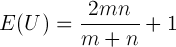
- The test which will be used to check stationarity is the Runs Test (or Wald-Wolfowitz test). The Runs Test was developed by Wald and Wolfowitz (1940) to test the hypothesis that two samples come from the same population (see paragraph about ergodicity below). Particularly the extension that uses the Runs Test to test the fitness of a given function will be employed (Gibbons 1985). Given a time series and a function that is meant to explain the time series, the observations should be randomly distributed above and below the function if the function fits the time series, regardless of the distribution of errors. The Runs Test tests whether the null hypothesis of randomness can be rejected or not. Given the estimated function, a 1 is assigned to the observations above the fitted line, and a 0 to the observations below the fitted line (where 1 and 0 are considered as symbols). Supposing that the unknown probability distribution is continuous, probability will be 0 that a point lies exactly on the fitted line (if this occurs that point should be disregarded). The outcome of the described process is the sequence of ones and zeros that represents the sequence of observations above and below the fitted line. The statistics used to test the null hypothesis is the number of runs, where a run is defined as "a succession of one or more identical symbols which are followed and preceded by a different symbol or no symbol at all" (Gibbons 1985). For example in the sequence 1,0,0,1,1,1,0 there are 4 runs ({1},{0,0},{1,1,1} and {0}). The number of runs, too many or too few runs, may reflect the existence of non-randomness in the sequence. The Runs Test can be used with either one or two sided alternatives[3] (Gibbons 1985). In the latter case the alternative is simply non-randomness, while the former (with left tail alternative) is more appropriate in the presence of trend alternatives and situations of clustered symbols, which are reflected by an unusually small number of runs. Following Wald and Wolfowitz's notation (1940), the U-statistic is defined as the number of runs, m as the number of points above the fitted function and n as the points below the fitted function. The mean and variance of the U-statistic under the null-hypothesis are
(1) 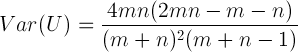
(2) The asymptotic null-distribution of U, as m and n tend to infinity (i.e. as the number of observations tends to infinity) is a normal distribution with an asymptotic mean and asymptotic variance. In the implementation of the test, exact mean and variance (1) and (2) are used to achieve better results with few observations and equivalent results with many observations. The derivation of the finite sample properties and of the asymptotic distribution of U is reported in the literature (Wald and Wolfowitz 1940; Gibbons 1985). To conclude, the Runs Test tests the null-hypothesis that a given set of observations is randomly distributed around a given fitted function; it tests whether the fitted function gives a good explanation of the observations.
- 2.4
- The idea is to use the test described above to check the stationarity of a time series. Defining the moment of order k as the non-centered moment of order k:
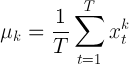
(3) and supposing that we have an agent-based model, we want to test the stationarity of a given set of moments of the artificial time series. We may be interested in the behavior of the moments to compare them to some real data, or we may use the moments to analyze the behavior of the model under different conditions. In any case it is necessary to know whether the estimation of the artificial moment of order k is consistent (i.e. if it reflects the behavior of the model). In order to check whether a moment is stationary, we have to check whether the moment is constant in time. The first step is to divide a time series produced with the model into w windows (sub-time series). Then the moment of order k for each window is computed. If the moment of order k is constant, the "window moments" are well explained by the moment of the same order computed over the whole time series ("overall moment"). To test the hypothesis of stationarity the Runs Test is used: if the sample moments are fitted by the "overall moment" (i.e. if the sample moments are randomly distributed around the overall moment), it is concluded that the hypothesis of stationarity for the tested moment cannot be rejected. A strictly stationary process will have all stationary moments, while a stationary process of order k in this framework means that the first k non-centered moments are constant.
- 2.5
- To run the test, the length of the time series and the length of the windows must be decided. Under the null hypothesis, longer windows imply a better estimation of the subsample moments, but at the same time they imply fewer windows (given the length of the time series) and a worse approximation of the distribution of runs toward the normal distribution. The trade off can be solved by using long series and long windows. In the following, Monte Carlo experiments will be made to check the performance of the test; in particular a time series of 100000 observations will be used, and the performance of the test on 100 processes will be checked. The following window lengths will be used[4]: 1, 10, 50, 100, 500, 1000, 5000, 10000. By changing the length of the windows the number of samples is changed (since the length of the time series is fixed). The experiments will check the stationarity of the moment of order 1 (mean) of an autoregressive function of the first order:
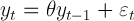
(4) with θ=0 (strictly stationary), θ=0.99 (stationary), and θ=1(non-stationary), and εt a random error with uniform distribution U(-1,1). The experiments have been carried out using the two-tail test. In figure 1 is shown an example of a strictly stationary process (θ=0) with the overall mean and the window means (the window length is 10). In figure 2 an example of a nonstationary process (θ=1) is shown together with its overall and window means. The different behavior of the first moment in the two different processes is clear. The test assigns a 0 to the window moments below the overall moment and a 1 to the window moments above the overall moment. The different behavior of the two processes is detected by the test from the different number of Runs. In figure 1 the overall mean is a good estimator of the window means (and the null-hypothesis cannot be rejected), in figure 2 the overall mean is not a good estimator of the window means (the null-hypothesis is rejected).
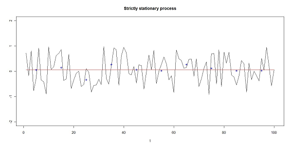
Figure 1. An example of the process (4) with θ=0 and y0=0. The black line is the time series, the red line is the overall mean, the blue dots are the window means (shown in the middle of the windows, the window length is 10). In a stationary series the window moments are randomly distributed around the overall moment. 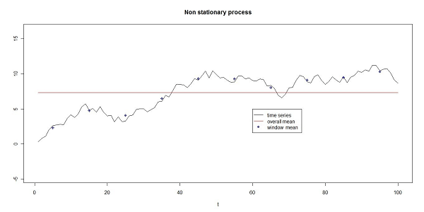
Figure 2. An example of the process (4) with θ =1 and y0=0. The black line is the time series, the red line is the overall mean, the blue dots are the window means (shown in the middle of the windows, the window length is 10). The overall mean is not a good estimator of the window means, the test detects non-stationarity due to the small number of runs (the number of runs defined on the window moments is only 2 in this example). 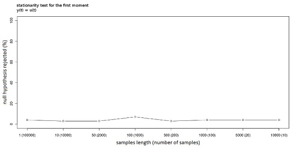
Figure 3. Stationarity null-hypothesis rejected (%) with different window lengths. The process is stationary. 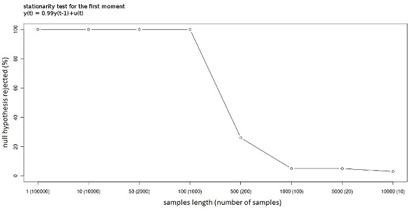
Figure 4. Stationarity null-hypothesis rejected (%) with different window lengths. The process is stationary. 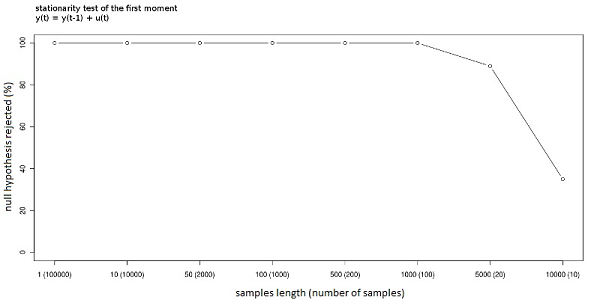
Figure 5. Stationarity null-hypothesis rejected (%) with different window lengths. The process is non stationary. - 2.6
- Figures 3, 4 and 5 show the result of Monte Carlo simulations of the test on the first moment using the process defined in (4) with different values of θ. The null hypothesis is that the first moment is constant, and in turn that the sub-time series of moments are fitted by the overall first moment. Since a type-I error[5] equal to 0.05 is being used, we will find that the null hypothesis is rejected when the null is true in 5% of the cases; this occurs with both θ= 0 and θ = 0.99. It is interesting to note that the length of the windows has no influence when the process is strictly stationary. Particularly, if every observation has the same distribution, the stationarity can be detected even when the window length is equal to 1. However, if θ=0.99, longer windows are needed to detect the stationarity property in order to allow the sub-time series to converge toward the overall mean; in other words more observations are needed to obtain a good estimation of the subsample moments. Non-stationarity is also simple to detect; the test has full power (it can always reject the null when the null is false) for all the window lengths except the ones that reduce the number of windows under the threshold of good approximation of the normal distribution (the test has power 1 as long as the number of samples is more than 50). According to the experiments, the best option seems to be a window of length 1000 (given the length of the whole time series) that permits both the estimation of the subsample moments and at the same time the convergence of the distribution of the runs toward the normal distribution. The test has to be repeated for every needed moment. Figure 6 shows how the first and second window moments (the dots) behave in a time series produced by a process as described in (4) with θ=0 and with an error term that has a distribution of U(-1,1) in the first part of the time series and a distribution of U(-8,8) in the second part. The test outcome is (correctly) stationarity of the first moment and non-stationarity of the second moment. The "overall second moment" does in fact not fit the subsample second moments, and the test can detect this lack of fit caused by the limited number of runs (only two in this case).
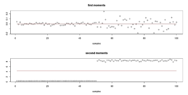
Figure 6. The dots are the window moments, the line is the overall moment. The first moments are randomly distributed around the overall mean (above). The second moments are not randomly distributed around the overall moments (below). - 2.7
- The experiment shows the flexibility and the limits of the test: we can—and must—test the moments we need. If the length of the time series and the number of windows are properly set, the result stating stationarity for the tested moment is reliable, i.e. the power of the test approaches 1, while the actual type-I error is around 5%. If non-stationarity is found, the traditional methods may be used to transform the series into stationary (for example detrending or differentiating the series) and the nonparametric test can then be used on the transformed series.
Ergodicity
- 3.1
- Ergodicity, together with stationarity, is a fundamental property of a data generator process. Hayashi (2000) gives the following formal definition of ergodicity: a stationary process {yt} is said to be ergodic if for any two bounded functions f:Rk → R and g:Rl →
R,

(5) Heuristically, this means that a process is ergodic if it is asymptotically independent: two distant observations are almost independently distributed. If the process is stationary and ergodic the observation of a single sufficiently long sample provides information that can be used to infer about the true data generator process and the sample moments converge almost surely to the population moments as the number of observations tend to infinity (see the Ergodic Theorem in Hayashi 2000, p. 101). Ergodic processes with different initial conditions (and in agent-based models, with different random seeds) will thus have asymptotically convergent properties, since the process will eventually "forget" the past.
- 3.2
- Ergodicity is crucial to understanding the agent-based model which is being analyzed. If the stationarity test reveals the convergence of the model toward a statistical equilibrium state, the ergodicity test can tell whether such equilibrium is unique. Supposing that we want to know the properties of a model with a given set of parameters, if the model is ergodic (and stationary) the properties can be analyzed by using just one long time series. If the model is non-ergodic it is necessary to analyze the properties over a set of time series produced by the same model with the same set of parameters but with different random seeds (that is with a different sequence of random numbers). It is even more important to take ergodicity into consideration if the model is compared with real data. If the data generator process is non-ergodic, the moments computed over real data cannot be used as a consistent estimation of the real moments, simply because they are just one realization of the data generator process, and the data generator process produces different results in different situations. A typical example of a stationary non-ergodic process is the constant series. Supposing for example that a process consists of the drawing of a number y1 from a given probability distribution, and that the time series is yt = y1 for every t. The process is stationary and non-ergodic. Any observation of a given realization of the process provides information only on that particular process and not on the data generator process. Despite the importance of the ergodicity hypothesis in the analysis of time series, the literature about ergodicity tests is scarce. Domowitz and El-Gamal (1993; 2001) describe a set of algorithms for testing ergodicity of a Markovian process. The main intuition behind the test is the same as the one used in this paper: if a data generator process is ergodic it means that the properties of the produced time series (as the number of observations goes to infinity) is invariant with respect to the initial conditions. The test described below is different from the one described by Domowitz and El-Gamal (1993) since it involves different algorithms, uses a different nonparametric test and is intended to be used directly on any computational model (an example of application to a simple agent-based model will be shown in section 4). The algorithm basically creates two samples representing the behavior of the agent-based model with different random seeds and compares the two samples using the Wald-Wolfowitz test (Wald and Wolfowitz 1940). There are a number of alternative nonparametric tests that could have been used such as the Kolmogorov-Smirnov test (used by Domowitz and El-Gamal 1993) and the Cramer-Von Mises test (for references about nonparametric tests see for example Darling 1957, Gibbons 1985 and Gibbons and Chakraborti 2003). The Wald-Wolfowitz test was chosen due to its simplicity and to the fact that under the null-hypothesis the test statistic is asymptotically distributed as a Normal, which implies an easy implementation with most statistical and numerical software and libraries (in this paper the Rpy library for Python was used).
- 3.3
- The test described below is a test of ergodicity of the moment of order k; it tests the invariance of the moment of order k between different processes produced by the same data generator process with different random seeds. The ergodicity test says if the first moments (for example) of a series can be used as the estimation of the true moment of the data generator process. It is necessary to replicate the test for every moment required.
Ergodicity Test
- 3.4
- To test the ergodic property of a process, the Run Test is used again, but this time in the original version presented by Wald and Wolfowitz (1940) to test whether two samples come from the same population. Wald and Wolfowitz's notation is used supposing that there are two samples {xt} and {yt}, and supposing that they come from the continuous distribution f(x) and g(x). Z is the set formed by the union of {xt} and {yt} and the Z set is arranged in ascending order of magnitude. Eventually, the V set is created, i.e. a sequence defined as follows: vi=0 if zi ∈{xt} and vi=1 if zi∈{yt}. A run is defined as in the previous section and the number of runs in V, the U-statistic, is used to test our null hypothesis f(x)=g(x). In the event that null is true, the distribution of U is independent of f(x) (and g(x)). A difference between g(x) and f(x) will tend to decrease U. If m is defined as the number of elements coming from the sample {xt} (number of zeros in V) and n as the number of elements in Z coming from the sample {yt} (number of ones in V), m+n is by definition the total number of observations. The mean and the variance of the U-statistics are (1) and (2). If m and n are large, the asymptotic distribution of U is a Normal distribution with the asymptotic mean and the asymptotic variance (as in the stationarity test, the exact mean and variance to implement the test are used). Given the actual number of runs, U, the null hypothesis is rejected if U is too low (U is tested against its null distribution with the left one-tailed test). In this case the aim is to use this test as an ergodicity test supposing that the stationarity test has not rejected the null hypothesis of stationarity. Under the null hypothesis of ergodicity, the sample of moments computed over the sub-samples of one time series has to come from the same distribution of the moments computed on many processes of the same length as the sub-samples. To test ergodicity of the first moment (or moments of higher order) one random long time series is created and divided into sub-samples. As shown in the previous paragraph, in order to have a good estimate of the sample moments 100000 observations can be used and divided into 100 sub-samples of 1000 observations each. The first sample (e.g. {xt} ) is formed by the moments of the first order of the 100 sub-samples. To create the second sample (e.g. {yt} ) 100 random time series are created (with different random seeds) of 1000 observations each, and the moment of the first order of each process is computed. Given the two samples the Runs Test can be used as described above. Under the null hypothesis, sample {xt} and sample {yt} have the same distribution. The moments of the two samples have to be computed over time series of the same length (in this case 1000). Under the null hypothesis, the variance of the moments depends on the number of observations used to compute the moments. For example, the use of very long time series to build the second sample would produce a sample of moments with a lower variance, and the Runs Test would consider the two samples as coming from different distributions.
- 3.5
- As regards the implementation of the test, it is worth noticing the case in which the time series converges during the simulation toward a long run equilibrium. If the number of observations is sufficiently long the stationarity test will correctly deem the process as stationary, whereas the ergodicity test will yield a non-ergodic outcome even if the process is ergodic. This result is due to the way the samples are produced. In figure 7 it is possible to see what happens; it shows the long process, the short process and the set of moments computed from the 100 sub-samples of the long time series (dots) and the moments computed over 100 different processes (squares). The need to keep the number of observations equal in the sub-samples and in the short processes creates the "convergence problem". Since the small processes used to build the second sample of moments do not have the time to reach the long run mean, the ergodicity test will detect non-ergodicity: it will find significant differences between the two samples.
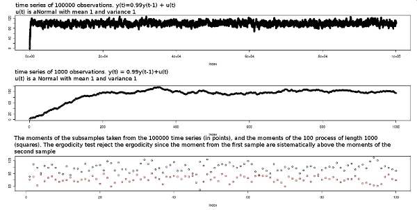
Figure 7. The long process (above), a short process (middle) and the moments computed from the subsamples of the long process (points) and the moments computed from the short processes (squares). The process used in figure 7 is yt=0.99yt-1+ut where ut ∼ N(1,1) and y0=0. The process is stationary and ergodic; it starts from zero and converges toward the asymptotic mean E(yt)=100. The ergodicity test will fail, since the two samples are clearly different (see bottom of figure 7). A strategy to solve this problem is to select a set of observations of the length of the sub-samples in a region where the time series has already converged to the long run mean. For example, to build the second sample a set of time series with 2000 observations can be created and the moments using the last 1000 observations can be computed.
- 3.6
- To check the performances of the test a Monte Carlo simulation testing the ergodicity of the first moment is performed using the following process[6]:
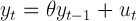
(6) where ut ∼ N(l,1) and l is a random variable distributed as U(-5,5). At the beginning of the process a draw of l will determine the expected value of ut for the whole process. If the process (6) is stationary, i.e. |θ|< 1, the value of l determines the equilibrium state of the process. The stationarity test on the first moment would, in this case, detect the presence of an equilibrium state, while the ergodicity test on the first moment will detect whether the equilibrium is unique (given θ). Figure 8 shows different examples of the process (6) with different values of l, with y0=0 and θ = 0.9. It is clear that the process converges toward a different equilibrium state depending on the value of l.
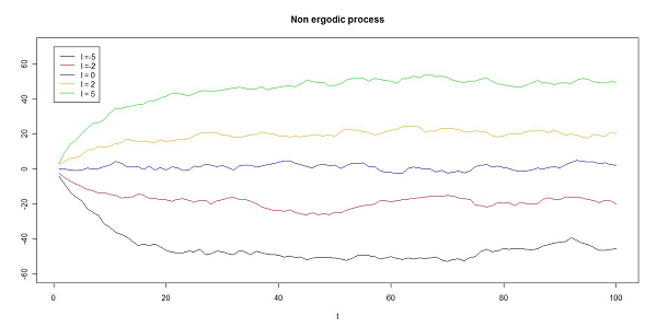
Figure 8. Different initializations of the process (6). The value of l extracted at the beginning of the process determines the equilibrium state of the process. The process is stationary (has an equilibrium state) and non-ergodic (given θ the process has multiple equilibrium depending on the value of l). - 3.7
- The process is ergodic if l is always the same for any initialization of the process. The aim of the process defined in (6) is to replicate a situation in which the starting condition has an everlasting effect on the process. By isolating the convergence problem using the method described above[7], the test performs exactly in the same way whether an ergodic process has a convergence phase or not. These performances are shown in the first part of figure 9 where the process defined in (6) was tested with initial condition y0=0 and with different values of θ . When θ = 0 and θ= 0.99 and the processes are ergodic the test on the first moment gives non-ergodicity results in about 5% of cases (due to the type-I error) but if the process is non-stationary,θ=1, the test gives 100% non-ergodicity results (as stated before, the ergodicity test needs a stationary process to work).
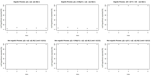
Figure 9. Ergodicity test performances (% of rejection of the ergodicity null hypothesis under different conditions). The test on the first moment for an ergodic process (above) and the test on the first moment for a non-ergodic process (below). One experiment is made by testing the same process100 times using different random seeds. The experiment was done 5 times for each setting. - 3.8
- The second part of figure 9 shows the test on the first moment made on a non-ergodic process (note that the process defined in (6) is non-ergodic in the first moment), where an initial random draw determines the asymptotic mean of the process. Since y0 is fixed, the technique described above has been used to solve the convergence problem. In this way it is certain that there is no bias in the test (if the convergence problem had not been overcome, the result would have been non-ergodicity also in case of ergodicity and it would not have been possible to exclude the possibility that the high power of the test was due to the convergence problem). The test can detect non-ergodic processes with power 1. In order to clarify how the test works, the two samples built to make the test for an ergodic (above) and a non-ergodic process (below) are shown in figure 10. From a simple graphic analysis it is possible to see intuitively how the two samples come from the same distribution in case of an ergodic process; while there is a difference in case of non-ergodicity (the dots are the first sample, while the squares are the second sample).
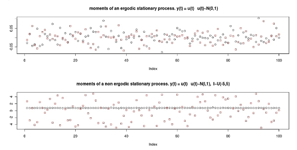
Figure 10. The test checks whether there is a significant difference between the two samples of moments. The two samples in the case of ergodicity (above) and the two samples in the case of non-ergodicity (below). The dots are the moments coming from the first sample (built with the moments of the subsamples of the long series) and the squares are the moments coming from the second sample (built with the moments of the short processes). The process is as in (6) with θ= 0. The test can detect whether there is a significant difference between the two sets of moments. This is a test of invariance of the mean between different processes; if the test is passed the mean of an observed series can be used as a consistent estimator of the true mean. The process may be ergodic in the first moment but non-ergodic in the second moment. To analyze the performance of the test in case of a non-ergodic second moment the same setting as before is used (6) with ut∼ N(0,l). If the process is non-ergodic, the variance of the error changes in different processes, l∼ U(1,5). In this case it is necessary to test the ergodicity of both the first and the second moment (as defined above). In order to test the second moment, the first sample is built using the second moment of the 100 subsamples and the second sample using the second moment of the 100 processes. The test is exactly as above but comparing second moments. Given a model that produces the data following the process (6) with the new error term, and provided that the process is stationary and non-ergodic, the outcome of the test of ergodicity on the first moment yields between 20% and 30% of non-ergodicity results. This is because the different variance of the error implies a different variance in the first moments, so despite the fact that the different processes have the same mean, the test detects that "something is wrong". Given such a result it is necessary to test for the ergodicity of the second moment. The outcome of the test (on the second moment) on a (second moment) non-ergodic process yields 100% of non-ergodic results (the power is 1). The result of the test on an ergodic stationary process gives about 5% of non-ergodicity results, which is the chosen type-I error.
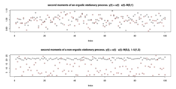
Figure 11. The two samples of second order non-centered moments in the case of ergodicity (above) and non-ergodicity (below). In figure 11 the (second) moments in the first and the second samples for an ergodic process (with error term ut ∼ N(0,1)) and the (second) moments in the first and in the second sample for a non-ergodic process (with error term ut ∼ N(0,l) and l ∼ U(1,5), l is fixed at the beginning of the process as it depends on the "initial conditions"), in both figures the process is as in (6) with θ=0.
Using the tests on a simple agent-based stock market
- 4.1
- In this section a partially modified version of the computational stock market proposed by Gode and Sunder (1993) will be presented and analyzed[8]. The aim is to use the tests on an actual (even if very simple) agent-based model. Gode and Sunder (1993) propose a computational stock market model where the agents have very limited cognitive abilities. The objective is to compare an experimental stock market with human subjects to a computational stock market with two different types of agents. The intention is to reproduce the result of the experiment in a completely controlled computer environment. The problem of experimental economics is that it is possible to control the environment, but it is not possible to control the effect of the behavior of the agents. Using agent-based modeling, the behavior of the agents is completely formalized as an algorithm and it is possible to check the behavior of the system with different types of agents. Following the well-known experiment described in Smith (1962), Gode and Sunder (1993) make an experiment in which they randomly divide the subjects in buyers and sellers, provide each trader with a private value (known only to the trader) for the fictitious commodity traded in the stock market. The subjects were free to submit orders at any time, conditioned only by their assigned role and by their private value. The interesting results described by Smith (1962) and replicated in Gode and Sunder (1993) is the fast convergence of the transaction price toward the theoretical equilibrium, defined by the demand and supply schedules induced by the experimenter. The market is highly efficient, despite the low number of traders and the private nature of the evaluation of the fictitious commodity. Gode and Sunder (1993) built a computational market organized as a continuous double auction. The behavior of the market with human subjects is compared to the computational market with Zero-Intelligence (ZI) traders and with Zero-Intelligence Constrained (ZI-C) traders. The ZI traders made orders only conditional to their role choosing a price randomly between 1 and 200. The ZI-C traders made orders conditional both to their role and to their private value. The chosen price would be a random value between the private cost and 200 for the sellers and between 1 and the private value for the buyer. Gode and Sunder (1993) interpreted the constraint as imposed by the market mechanism: "Market rules impose a budget constraint on the participant by requiring traders to settle their account" (Gode and Sunder 1993, p. 122). The astonishing result is that the efficiency of the market increases dramatically with the imposition of constraints on the traders' behavior. Gode and Sunder (1993) conclude that what really matters in the observed convergence of the price toward the theoretical equilibrium in the experiment are the market rules, while the rationality and profit-seeking behavior of human traders can account only for a small fraction of the efficiency of the market (this conclusion has been criticized, see in particular Gjerstad and Shachat 2007 and Cliff and Bruten 1997). The model presented below is very similar to the Gode and Sunder (1993) model[9]. There are 22 artificial traders divided in two groups: sellers and buyers. Each seller is given a number representing the cost and each buyer is given a number representing the value of the traded asset. Values and costs are private information. The trading is divided into periods, in each period each trader is free to issue orders. When a deal is made the involved traders drop out from the market for that period. At the end of each period the order book is cleared. This division of time allows the definition of a demand schedule and a supply schedule for each time period and therefore the definition of the theoretical equilibrium of the market (see Smith 1962). In figure 12 the demand and supply schedules, the market price over 10 periods with ZI agents and the market price over 10 periods with ZI-C traders are shown. The volatility of the price is heavily reduced and the market price fluctuates around the theoretical equilibrium even if the agents behave (almost) randomly.
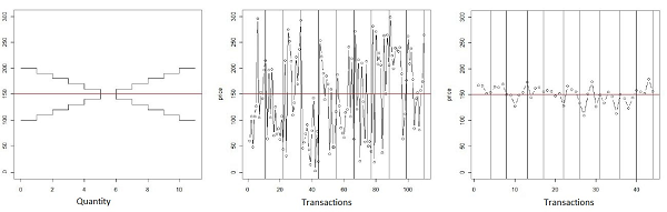
Figure 12. From left to right: the per period demand and supply schedules defined by the private values and costs given to the traders; the transaction price in a market with Zero-Intelligence traders; the transaction price in a market with Zero-Intelligence Constrained traders. The vertical lines in the central and right figures refer to the periods. - 4.2
- The aim is to test whether the model with ZI-C traders is stationary and ergodic. The method that will be used is the one described in previous sections and the test will be made on the first moment. The Monte Carlo experiments performed in section 2 on a process with known properties showed that to have a test with full power in the stationarity test it is necessary to have a minimum number of windows (at least 50, to have a good approximation of the distribution under the null-hypothesis). On the other hand, the length of the windows is important to detect stationarity when the process is weakly stationary. The stationarity test is performed over time series with 2500 observations using windows with a length of 1, 10, 30 and 50. The results are in figure 13. The rejection rate for 100 simulations for each of the window lengths is coherent with the chosen type-I error (5%), it is therefore not possible to reject the null hypothesis of stationarity. The test is not rejecting stationarity even with windows of length 1, a result which allows inferring that the transaction price is strictly stationary[10].
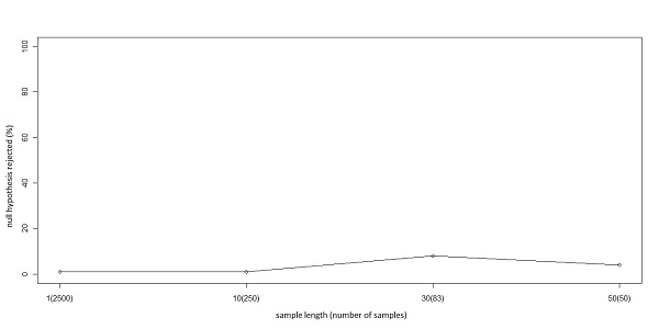
Figure 13. The % of rejections of stationarity null-hypothesis with different window lengths made on the stock market model. - 4.3
- The ergodicity test is carried out as described in section 3. A long time series is created and divided into windows, and the first moment of each window is computed. Given the stationarity test we know that the expected value of each window is the same, and therefore we know that the sample moment computed over each window comes from the same distribution, with a mean value equal to the expected value and variance depending on the variance of the process and on the length of the windows. The aim of the ergodicity test is to test whether the model shows the same behavior when the initial conditions are changed. The ergodicity test will therefore compare the set of moments computed over the windows of one long time series (sample 1) with a set of moments computed over a set of different runs of the same model with different random seeds (sample 2). Under the null-hypothesis of ergodicity sample 2 comes from the same distribution as sample 1, the test is made using the Wald Wolfowitz test. The ergodicity test is performed using one long time series of 1000 observations divided into 100 windows with length 10 to form sample 1. Sample 2 is created by running the model 100 times with different random seeds with a length of 10 observations. The Wald-Wolfowitz test compares the two samples and cannot reject the null hypothesis, i.e. the model is ergodic. The 100 tests present a rejection rate of 5%, a result that is coherent with the chosen type-I error (5%). The results of the tests are that the model is stationary and ergodic.
- 4.4
- It is also possible to modify the model in order to make it non-ergodic[11]. From the analysis of the behavior of the model we know that the mean transaction price—the equilibrium since it is stationary—depends on the private values of the agents. In the ergodic version of the model the agents arrive on the market with an evaluation of the traded commodity. A non-ergodic version of the model can be built by supposing that the traders arrive on the market with a confused evaluation of the commodity and that they wait in order to observe the behavior of the other traders before they decide how to trade. In behavioral terms it can be explained as an anchoring behavior (Tversky and Kahneman 1974), i.e. the traders look for information in the environment (for example observing the actions of the other traders) before they decide how to behave. If the anchoring happens only once at the beginning of the trading day the market is stationary (there is an equilibrium) but non-ergodic since the particular value of the equilibrium depends on the anchoring value (that will be simply represented as a random draw at the beginning of the market day). To give a quantitative evaluation of the statistical properties of the model the ergodicity test is used. Suppose that the first trader is a buyer and that she arrives on the market and draws her private value v ∼U(200,300). The next buyer arrives on the market and chooses a value equal to that of the buyer who arrived before her minus 10, in this way the demand function is created. To keep the market simple the demand and supply schedules are symmetric, therefore the costs of the sellers are given according to the values of the buyers (figure 12 shows an example of symmetric market). The market is non-ergodic since its equilibrium depends on the initial condition and in particular on the value of the first buyer that arrives to the market. The maximum value of the equilibrium price is 250 and the minimum value is 150. The equilibrium price is distributed as a U(150,250) due to the distribution of the random variable that determines the first value. The average equilibrium is thus 200 and the variance of the equilibrium is 833.3.
- 4.5
- The test was performed with the same parameters of the previous ergodicity test (the length of the long time series is 1000 and the length of the windows and of the short time series is 10) and the result is the rejection of the ergodicity null-hypothesis. In 100 tests the null is rejected 100% of the times (full power). Figure 14 shows two markets with different initial conditions.
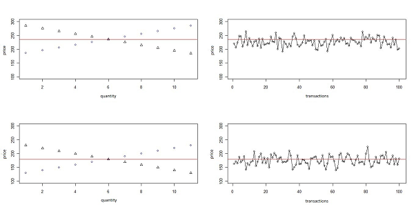
Figure 14. Two realizations of the non-ergodic stock market. On the right the realized demand and supply schedule, on the left the first 100 transactions are shown. - 4.6
- The main drawback of agent-based models is that it is not possible to prove formally the properties of the model. Even in a model as simple as the described artificial stock market, the equilibrium properties cannot be formally proven. The aim of the tests is to reduce the problem using statistics over the artificial data. The test allows a quantitative and statistical assessment of the properties of the model, and thereby of the economic properties of the model. Knowing that the model has (or does not have) a unique stable equilibrium is essential both for understanding the behavior of the model and for understanding the system under analysis. The stationarity test is thus useful to confirm statistically that the model has an equilibrium state and the ergodicity test allows to know whether the equilibrium is unique regardless of the initial condition. Given the properties of the model, supposing that it has been built to represent a real system, it is possible to use the results of the tests performed on artificial data to infer about the real data. In the present case the model is far too simple to represent any real stock market, but if it had been a real stock market we would have discovered that the transaction price is stationary and ergodic. While the stationarity can be tested also on the real data, the ergodicity test can be performed only on the artificial data. If the model is well-specified, a sufficient number of observations from the real system are available and if the model (i.e. the real data) is stationary and ergodic, then it is possible to consistently estimate/calibrate the model (see Grazzini 2011a). Given the result of the test carried out on the model it is possible to perform the sensitivity analysis with a better knowledge of its basic properties.
Conclusions
- 5.1
- This paper has presented an algorithm using the Wald-Wolfowitz test to detect stationarity and ergodicity in agent-based models. The tests were evaluated using the Monte Carlo method. Knowing whether a model is ergodic, and when its output becomes stationary is essential in order to understand its behavior. The stationarity test can help to detect the point where a system reaches its statistical equilibrium state by using not only a visual and qualitative inspection, but also a quantitative tool. The ergodicity test provides a rigorous base to the analysis of the behavior of the model (see Grazzini 2011b). Any comparison between different settings of the model, or between different policies, should be based on the knowledge about the ergodicity property. If a model is not ergodic, it makes no sense to perform a sensitivity analysis over the parameter space with a given random seed. The tests are crucial also in view of a comparison between the properties of the model and the properties of the real system. It is always possible to use real data to "calibrate" an agent-based model, but if the system is non-ergodic, the parameters of the model cannot be properly estimated (Grazzini 2011a).
- 5.2
- In view of this, a nonparametric test is required due to the practical impossibility to understand how the random component influences the emergent properties of the model in many agent-based models. While nonparametric tests on real data often lack power, this problem disappears when the tests are applied to simulated data to investigate the properties of a theoretical model: by increasing the number of observations their power can be increased at will.
Acknowledgements
- I would like to thank three anonymous referees, as well as Matteo Richiardi and Pietro Terna, for their stimulating comments on earlier versions of the paper.
Notes
-
1 The Python random library has been used for the generation of the pseudo random numbers. The algorithm is the Mersenne Twister which produces 53-bit precision floats and has a period of 219937-1.
2 If the model is stationary and ergodic (see section 3) then the observed sample carries information about the true data generator process (which is always the same for any initial conditions).
3 If the null-hypothesis is true the test statistic has a known distribution. The null-hypothesis is rejected if the actual test statistic (computed over the observations) is too far away from the null-hypothesis, where "too far" is defined relatively to the null-distribution and the chosen type I error (the type I error is defined as the probability of rejecting the null-hypothesis when the null is true). The test can be made either with a two-sided alternative (the null is rejected both if the actual test statistic is too big or too small) or a one-sided alternative (the null is rejected if the actual test statistic is either too big, right alternative, or too small, left alternative). Left side alternative means that the null-hypothesis is rejected only if the actual test statistic is too small.
4 The test is coded in Python. The Python module required for the use of the the test can be downloaded from the internet site http://jakob.altervista.org/nonparametrictest.htm
5 Type I error is the probability of rejecting the null-hypothesis when the null-hypothesis is true.
6 The test is coded in Python. The Python module required for the use of the test can be downloaded from the internet site: http://jakob.altervista.org/nonparametrictest.htm
7 Use a set of observations chosen from the stationary part of the process
8The Python modules of the model and the tests can be downloaded from http://jakob.altervista.org/GodeSunderErgodic.rar
9 The first difference is that the ZI traders generate offers and bids using a uniform random variable between 0 and 300 (instead of 1 and 200). The ZI-C traders use a random value between the private cost and 300 for the sellers and between 0 and the private value for the buyers. The results are the same. Other differences are in some trading rules. For example Gode and Sunder (1993) use resampling: they force every agent to issue a new order after each transaction (see LiCalzi and Pellizzari 2008).
10The overall mean computed on the 2500 observations is 150.04, very similar to the theoretical equilibrium.
11 The Python modules of the non-ergodic version of the model and of the tests can be downloaded from http://jakob.altervista.org/GodeSunderNonErgodic.rar
References
-
CLIFF, D. and Bruten, J. (1997). Minimal-intelligence agents for bargaining behaviors in market based environments, HP Laboratories Bristol (HPL-97-91).
DARLING, D.A. (1957). The Kolmogorov-Smirnov, Cramer-Von Mises tests, The Annals of Mathematical Statistics 28(4), 823-838. [doi:10.1214/aoms/1177706788]
DICKEY, D.A. and Fuller W.A. (1979), Distribution of the estimators for autoregressive time series with unit root, Journal of the American Statistical Association 74 (366), 427-231. [doi:10.2307/2286348]
DICKEY, D.A. and Fuller W.A. (1981). Likelihood ratio statistics for autoregressive time series with a unit root, Econometrica 49(4), 1057-1072. [doi:10.2307/1912517]
DOMOWITZ, I. and El-Gamal, M.A. (1993). A consistent test of Stationarity-Ergodicity. Econometric Theory 9(4), 589-601. [doi:10.1017/S0266466600007994]
DOMOWITZ, I. and El-Gamal, M.A. (2001). A consistent nonparametric test of ergodicity for time series with applications. Journal of Econometrics 102, 365-398. [doi:10.1016/S0304-4076(01)00058-6]
GIBBONS, J. D. (1985). Nonparametric Statistical Inference. New York: Marcel Dekker Inc., second ed.
GIBBONS, J. D. and Chakraborti S. (2003). Nonparametric statistical inference. New York: Marcel Dekker Inc.
GILLI, M. and Winker, P. (2003). A global optimization heuristic for estimating agent-based models. Computational Statistics and Data Analysis 42. [doi:10.1016/S0167-9473(02)00214-1]
GJERSTAD, S. and Sachat, J. M. (2007). Individual rationality and market efficiency, Institute for Research in the Behavioral, Economic and Management Science (1204).
GODE, D.K. and Sunder S. (1993). Allocative Efficiency of Markets with Zero-Intelligence Traders: Markets as a Partial Substitute for Individual Rationality. The Journal of Political Economy 101(1)119-137. [doi:10.1086/261868]
GRAZZINI, J. (2011a), Estimating Micromotives from Macrobehavior, Department of Economics Working Papers 2011/11,University of Turin
GRAZZINI, J. (2011b), Experimental Based, Agent Based Models, CeNDEF Working paper 11-07 University of Amsterdam.
HAYASHI, F. (2000). Econometrics. Princeton: Princeton University Press.
KWIATKOWSKI, D., Phillips, P.C.B., Schmidt, P. and Schin Y. (1992), Testing the null hypothesis of stationarity against the alternative of a unit root. Journal of Econometrics 54, 159-178. [doi:10.1016/0304-4076(92)90104-Y]
LEOMBRUNI, R. and Richiardi, M. (2005). Why are economists sceptical about agent-based simulations? Physica A 355(1), 103-109. [doi:10.1016/j.physa.2005.02.072]
LICALZI, M. and Paolo Pellizzari (2008). Zero-Intelligence trading without resampling. Working Paper 164, Department of Applied Mathematics, University of Venice. [doi:10.1007/978-3-540-70556-7_1]
PHILLIPS, P.C.B. (1987). Time series regression with unit root, Econometrica 55(2), 277-301. [doi:10.2307/1913237]
PHILLIPS, P.C.B. and Perron, P. (1988). Testing for unit root in time regression, Biometrika 75(2), 335-346. [doi:10.1093/biomet/75.2.335]
PHILLIPS, P.C.B. and Xiao, Z. (1998). A primer on unit root testing, Journal of Economic Surveys 12(5) 423-470. [doi:10.1111/1467-6419.00064]
RICHIARDI, M., Leombruni, R., Saam, N. J. and Sonnessa, M. (2006). A common protocol for agent-based social simulation. Journal of Artificial Societies and Social Simulation 9(1), 15. https://www.jasss.org/9/1/15.html.
SAID, S.E. and Dickey, D.A. (1984). Testing for unit roots in autoregressive-moving average models of unknown order, Biometrika 71(3), 599-607. [doi:10.1093/biomet/71.3.599]
SIEGEL, S. (1957). Nonparametric Statistics, The American Statistician, 11(3), 13-19.
SMITH, V. L. (1962). An experimental study of competitive market behavior, The Journal of Political Economy 70(2), 111-137. [doi:10.1086/258609]
TVERSKY , A. and Kahneman D. (1974). Judgment under Uncertainty: Heuristics and Biases. Science 185(4157), 1124-1131. [doi:10.1126/science.185.4157.1124]
WALD, A. and Wolfowitz, J. (1940). On a test whether two samples are from the same population. The Annals of Mathematical Statistics 11(2)147-162. [doi:10.1214/aoms/1177731909]