
 Abstract
- By means of a simulated funding-agency/supported-firm stochastic dynamic game, this paper shows that the level of the subsidy provided by a funding (public) agency, normally used to correct for firm R&D shortage, might be severely underprovided. This is due to the "externalities" generated by the agency-firm strategic relationship, as showed by comparing two versions of the model: one assuming "rival" behaviors between companies and agency (i.e., the current setting), and one associated to the "cooperative" strategy (i.e. the optimal Pareto-efficient benchmark). The paper looks also at what "welfare" implications are associated to different degrees of persistency in the funding effect on corporate R&D. Three main conclusions are thus drawn: (i) the relative quota of the subsidy to R&D is undersized in the rival compared to the cooperative model; (ii) the rivalry strategy generates distortions that favor the agency compared to firms; (iii) when passing from less persistent to more persistent R&D additionality/crowding-out effect, the lower the distortion the greater the variance is and vice versa. As for the management of R&D funding policies, we suggest that all the elements favouring greater collaboration between agency and firm objectives may help current R&D support to approach its social optimum.
- Keywords:
- R&D Subsidies, Rivalry Versus Cooperation, Dynamic-Stochastic Games, Simulations
Introduction
- 1.1
- It is commonly held that corporate R&D activities need to be subsidized. This occurs because many "market imperfections" might lead to an undersized R&D performance on the part of profit-maximizing enterprises. Generally, the literature has maintained that the "public good" attribute of knowledge (as R&D is approximately meant as a measure of knowledge production) and various other imperfections in markets for the financing of R&D are to be considered the main sources of this distortive phenomenon.
- 1.2
- Nevertheless, besides the overwhelming attention paid to explain the potential shortage of private R&D, the literature does not seem to have devoted so far comparable importance to the fact that also the level of public subsidies—decided at political level—could be severely underprovided. Indeed, it can be proved that this phenomenon could depend on two distinct (although correlated) characteristics of the "relation" between the funding agency and the supported units: (i) externalities generated by their strategic interaction, (ii) asymmetric information between agency and firms in assessing the quality of proposed R&D projects or in the level of effort provided by the firm in implementing the R&D objective. Although both are relevant aspects, the present paper abstracts from point (ii) while emphasizes the consequences of point (i) on both R&D and subsidy provision by means of a "simulated dynamic stochastic game" between a public agency choosing the level of R&D subsidies to be financed and a representative "supported" firm performing R&D.
- 1.3
- We set a forward-looking public agency choosing the time profile of subsidies by maximizing the average discounted sum of future values of an objective function assumed to be increasing in R&D (the agency wants to enlarge the national R&D outlay) and concave in the subsidy (as a budget constraint can be at work). Firms, on their part, maximize an instantaneous profit function (myopic assumption) in which R&D costs depend crucially on experience (accumulated R&D stock) and, of course, on subsidies received (plus other costs). At heart of the model there is the effect of the agency's subsidy on firm R&D activity's costs that is crucially modelled as a discrete Markov process with two potential states (positive or negative) to account for path-dependence in firm R&D "additionality" or "crowding-out" behavioural outcome.
- 1.4
- Solved computationally, two versions of the model are simulated and compared: one for the agency-firm "rival" strategy and one for the "cooperative" strategy (maximizing the sum of the two agents' objective function, that is, the "Pareto-efficient" strategy), under parameters set up according to model's internal coherence and some stylized facts. The crux of our analysis is the time pattern of the "ratio of subsidies on R&D expenditure" under different degrees of the persistency in the effect of the subsidy on firm R&D outlay. Nevertheless, the dynamic pattern of further endogenous variables such as R&D marginal costs and returns, stock of accumulated knowledge, agency and firm profits and social welfare is also explored.
- 1.5
- The paper is organized as follows: we first briefly review the literature on the rationale for R&D subsidization and present some related works using, as in our case, a simulation approach; in a subsequent section we present the structure of our model in terms of firm, agency and the cooperative behavioural assumptions, as well as a description of how we model the path-dependence of the subsidy effect in this context; a separate section is devoted to an explanation of the logical functioning of our model when embedded in a (pivotal) game theoretical perspective; then a specific section provides the main simulation results we obtain from running several times our stochastic model, while a final section closes the paper. Finally, the Appendix A placed at the end provides a "read-me" for the Matlab program used for performing the simulations.
Literature review
- 2.1
- The economic rationale for subsidizing corporate R&D is based on the idea that R&D activity owns some intrinsic characteristics that substantially differentiate it from other usual business activities. Jou and Lee (2001), for example, suggest that R&D is different from other private activities for three major reasons: (i) future rewards to R&D are extremely risky and uncertain, (ii) R&D spending takes the form of an irreversible choice (i.e., it generates hard sunk costs), (iii) R&D activities produce positive externalities. Within the literature, R&D subsidization was at the beginning invoked primarily for this third reason as accounted by the pioneering paper by Arrow (1962). The argument is well-known: since R&D activities have classical "public good" characteristics, the level of private R&D outlay would be systematically lower than the socially optimal level. This occurs since the benefits associated to R&D activities are easily and freely available to subjects that are not engaged in R&D efforts. As a consequence, the lack of full appropriability of R&D returns reduces the incentive to invest in knowledge on the part of private for-profit firms and thus government intervention is meant as an effective way to reduce the extent of this "market failure".
- 2.2
- Only recently, characteristics (i) and (ii) have been more seriously taken into account for justifying public intervention. In her extensive survey on the subject, Hall (2002) recognizes that, unlike externalities, other market failures associated to R&D activities can be relevant. For instance, when capital markets are imperfect, high-risk investments can severely suffer from credit rationing as the immaterial nature of R&D assets is unable to provide suitable collaterals to financers. In this case the asymmetric information between lenders and borrowers of R&D assets could be extremely high, thus generating higher rationing of funds. This problem is even more straighten in presence of financially constrained firms and undersized venture capital markets. The presence of high barriers to enter and exit the market is another potential source of private R&D shortage: on the one hand, when a great amount of irreversible R&D investment have been done by an incumbent firm, exiting the market could be seriously costly; on the other hand, entering the market could be difficult too as the R&D performed by incumbent firms (as well as their related patenting activity) may generate market power, thus weakening free access and competition from external companies (Dasgupta and Stiglitz 1980; Dasgupta 1988; D'Aspremont and Jacquemin 1988). Other motives suggesting the need for R&D support are based on the potential lack of technological infrastructures and bridging institutions, on coordination failure of profitable R&D joint ventures and on an excessive competitive arena leading to duplications in R&D efforts and other wastes of R&D-related resources (Mowery 1995; Metcalfe 1995; Malerba 1993; Martin and Scott 2000).
- 2.3
- No part of this literature has paid attention to the fact that also the R&D public intervention could be severely undersized and sub-optimally provided, although the aim of public support is to correct the market failures associated to low corporate R&D activities. Generally, public intervention is viewed in a Pigouvian perspective where the public agency is thought of as an independent, external and fully informed subject. In this perspective subsidies are thought of as "exogenous injections" rather than as an endogenous outcome of the strategic interplay between financing and financed subjects. Indeed, what we want to stress in this paper is that the public agency is an actor involved (strategically) in a game with financed companies, thus having its own objective function and behavioural strategy. The interaction between the public agency and the (financed) firm strategy generates an externality effect very similar to the Cournot-Nash type of the Prisoner's Dilemma or oligopolistic models, and it can be proved that this form of externality is responsible for an under-provision of the supplied subsidy.
- 2.4
- It is worth stressing, however, that in this paper we abstract from a second source of R&D subsidy sub-optimality, that caused by asymmetric information within public agency and financed companies. We only consider, within an optimal stochastic dynamic game, inefficiencies generated by strategic interaction thus ruling out those produced by potential moral hazard or adverse selection.
- 2.5
- As for previous literature on the subject, papers using a simulation approach for studying the effect of public subsidies on corporate R&D are very few and generally they do not model directly the public agency objective and behaviour. At micro-level papers of this kind are those by Jou and Lee (2001) and Laincz (2009). The latter embeds the R&D subsidization within a dynamic programming general equilibrium setting à la Ericson and Pakes (1995). The author builds a model with forward-looking dynamically optimizing firms where entry and exit decisions determine the dynamic of market structure. R&D subsidies are external interventions raising long-run growth rate and industry concentration as incumbent firms benefit more from them. Nevertheless, the funding-agency behaviour is not explicitly modelled and the R&D subsidy is just viewed as an external injection.
- 2.6
- At macro-level, Bental and Peled (2002) provide a calibrated dynamic model of growth in the spirit of endogenous growth models. They estimate the separate effect of restricted and unrestricted R&D subsidies on output and total factor productivity (TFP) growth, showing that both types of subsidies have significant long-run impact on aggregate performance. Yet, as in the case of Laincz (2009), no funding-agency decision process is represented in the model.
- 2.7
- The only paper we have found in the literature explicitly modelling the firm-agency subsidization relationship is that by Materia and Esposti (2009). This study is fairly close in spirit to our setting, although it is primarily interested in analysing only the optimal agency co-financing rate rather than a full set of endogenous variables as in our case. Moreover two important elements distinguish their work from that presented here: (i) it is essentially static as agency and firms maximize instantaneous objective functions, and (ii) it is fully deterministic. Our model, on the contrary, assumes agency's inter-temporal optimizing behaviour by also following a specific representation of the corporate R&D determination, the one proposed by Howe and McFetridge (1976). Furthermore our model is stochastic, pays specific attention to path-dependence and is primarily focused on welfare consequences of externalities generated by the agency-firm strategic interdependence.
The model
-
Firm behaviour
- 3.1
- Our model assumes a profit maximizing firm, choosing the optimal level of R&D investment by equating the marginal rate of return (MRR) and the marginal capital costs (MCC) of R&D as assumed in the model of R&D determination proposed by Howe and McFetridge (1976), subsequently drawn and revisited by David, Hall and Toole (2000), hereafter DHT[1]. The R&D rate of return (RR) is rtpt where rt are units of R&D expenditure and pt the marginal rate of return (MRR) to R&D. According to the DHT model, pt is assumed to be a decreasing function of rt. In the linear form we have that:
MRR: pt = φ0 - φ1rt with φ0, φ1 > 0 Where φ0 represents fixed marginal costs and φ1 a slope parameter controlling for the sensitivity of the MRR to firm R&D choice. The R&D investment capital cost (CC) is ctrt where ct is the marginal capital cost of R&D (MCC). It is assumed to depend (stochastically) on the level of the subsidy (st) and on the level of the R&D experience (kt, the R&D accumulated capital stock):
MCC: ct = μ - β At st - γ kt with β , γ > 0 Very concisely, this equation states that the unitary cost of doing R&D is a decreasing function of the R&D capital stock (in so accounting for a "learning by doing" phenomenon) and a function of st, the public subsidy, that has a positive impact (a cost reduction) when At is equal to 1 and a negative one (a cost increase) when At is equal to -1.
- 3.2
- The idea of letting At assume a negative effect, relies on some empirical findings. Indeed, although, at least in principle, we are more prone to assume that At may take only zero or positive values, empirical evidence have showed that the subsidy can have also "negative" effects on the R&D costs (thus increasing them). In a recent paper on the effect of R&D incentives on Italian manufacturing firms in Italy, for instance, Cerulli and Potì (2012) have found "more than full crowding-out" (negative R&D net change) for a number of subsidized companies. The authors proved that the median of the "average treatment effect on treated" (ATET) distribution is around zero: it means that half of the (supported) companies in their sample perform additionality, and the other half a crowding-out behaviour. The level of the R&D considered in that work is the "net R&D expenditure", equal to the total R&D performed minus the amount of subsidy received. Thus, it seems correct to account for a negative effect of the subsidy that is captured by a negative value of At.
- 3.3
- Nevertheless, the question is: why a subsidy can reasonably have a negative effect? According to a large body of case studies evidence, a negative effect seems to occur because of two possible causes (Potì and Cerulli 2011): (1) companies' co-financing requirement, and (2) delays, shortages and sub-provision of subsidies' allocation.
- 3.4
- As for point (1), we have to notice that generally companies may receive an R&D subsidy only under the requirement of covering part of the total R&D project costs by their own money. In other words, firms have to co-finance their R&D activity. Given this, if a firm is particularly internally liquidity-constrained and/or if accessing external funds turns out to be very costly, then the fact to have access to a public incentive might be even detrimental to R&D, because it exacerbates the liquidity constraint (internal and external) of the firm instead of reducing it. This may be a paradoxical but actual counter-effect of incentive schemes based on co-financing.
- 3.5
- As for point (2), we have to consider that R&D is primarily an "investment activity", whose effects are expected to take place in the future, not in the present time. As the investment theory suggests, investments are long-term expectation-based activities, where companies take into account strategic forward-looking elements. In this regard, company R&D activity should be seen as a programmed activity, entailing a multi-period planning strategy. Because of that, all the elements inducing expected uncertainty in the subsidy provision work as disincentives to do R&D. Factual experience proves that government delays in providing money, unexpected shortages of funds, as well as in-itinere reduction of negotiated subsidy amounts, can have serious negative effects on companies' propensity to do (planned) R&D. It means that a more than full crowding-out may be likely to take place.
- 3.6
- At is modelled as a Markov Chain stochastic process taking two states (+1 and -1) with a transition probability matrix depending on a parameter ρ (ranging from -1 and 1) accounting for the degree of "path-dependence". Indeed, when ρ = -1, At is a fully non-persistent process (and the minimum level of path-dependence is achieved), when ρ = 0, a uniform distribution of state transition probabilities over At is assumed, while when ρ = 1, At assumes +1 or -1 constantly (and the maximum level of path-dependence occurs). In this context the meaning of path-dependence deals with two crucial factors: (i) the persistency of successful/unsuccessful R&D projects proposed by firms, on the one hand, and (ii) the "selection" of supported units operated by the agency on the other. We will come to this point later on in the paper.
- 3.7
- The firm profit function associated to its R&D activity is:
πtF(rt,st) = rt pt - ct rt where we have put into evidence that it critically depends on its level of R&D (rt) and the level of the subsidy decided by the public agency (st) through ct. Given the level of the subsidy received from the agency, the firm chooses its optimal level of R&D expenditure (rt*) by maximizing its profit under the constrain represented by the law of motion of the R&D capital stock, that is:
rt* = argmax{π Ft = rt pt - ct rt}
s.t. rt = kt+1 - (1- δ )kt - 3.8
- Now, by simple algebra and deriving by rt, the previous system provides the optimal level of R&D expenditure as a function of At+1, st and kt+1, that is:
rt* = ξ ( φ0- μ ) + β ξ Atst + [ ξ γ /(1- δ )]kt+1 (1) This (analytical) formula explains the firm optimal R&D response to any level of the public subsidy, given the realization of the Markov process, the future level of knowledge stock and the choice of parameters' values. Observe that, according to the path-dependence argument we referred to above, the chain can generate a positive or negative effect of the subsidy on the optimal firm R&D expenditure. From equation (1) we get, by making st explicit and employing the R&D capital stock equation:
st = -(1/At)as - (1/At)bskt + (1/At)cskt+1 where as = ( φ0- μ )/ β , bs = (1- δ )/ β ξ , ξ = (1- δ )/[2 φ1(1 - δ ) + 2 γ ] , φ = (1- δ - ξ γ )/(1- δ ) and cs = φ/β ξ . Equation (2) turns to be the essential constraint under which the agency calculates the level of its subsidy provision in a dynamic programming environment. It is derived directly from the firm behaviour that the agency, in its turn, takes as given.
Agency behaviour
- 3.9
- The utility function of the agency is assumed to increase monotonically in rt while taking a quadratic concave form in st (inverted U-form). Indeed, while the agency profit should increase in rt as the agency wants the firm to produce as many R&D as possible, agency utility first increases in st and then, after a certain threshold (the maximum value), decreases in it.
- 3.10
- We argue that such a shape is in tune with the Managerial Utility Function Maximization Approach as proposed, for instance, by Williamson (1964). This theory challenged the traditional neo-classical holistic vision looking at organizations as profit-maximizing entities. Indeed, since the pioneering work by Berle and Means (1932), it was clearly recognized that organizations are owned by some shareholders (the citizens in the case of public agencies, the investors in company's stocks in the case of a private entities), but controlled by managers (Alchian and Demsetz 1972). Owners' and managers' interests might be substantially different, as managers have some discretion to use the organization's resources in their own interests. Organizations, thus, are heavily run in the interests of the managers. Williamson, among others, suggested that managers normally try to maximize their "satisfaction", by fixing ex-ante a given level of organizational performance to achieve. The utility of managers will be increased if their status improves by, for instance, an enlargement of staff expenditures (as this shows ability to manage), or if managerial salaries and profits are higher than an acceptable minimum level.
- 3.11
- The idea held in the paper is that the public agency providing R&D subsidies, is run by managers that might not act in the interest of the society as whole (the actual "owners" of the public agency). Thus, the aim of the managers is not that of maximizing social welfare, but their utility. Therefore, the agency utility is a concave function in st, that is, a function that assures that the agency's mangers have a (static) optimal level of st, given rt. The form of this function suggests that, as soon as the level of the subsidy increases, managers may get higher satisfaction, as they are able to enlarge their power and control capacity over the organization, and they are more likely able to obtain direct and indirect material and immaterial benefits. Moreover, since budget constraints are less binding for low level of st, an increasing shape of the agency's utility function for low level of st is fairly probable.
- 3.12
- Nevertheless, beyond a certain threshold, managing a too high amount of subsidy might be detrimental, as the level of the effort required to do this could become desperate. Furthermore, the presence of harsher budget constraints, due to the fact that the amount of R&D subsidies is generally limited and costly for the Government, bring pressure to managers to economize on it. Since managers need to be legitimated in front of the Government (entitled to set the amount of budget), they should be willing to act for that in Government's interests, at least to some acceptable extent.
- 3.13
- Therefore, the combination of these two effects: (i) managers' power satisfaction on the one hand, and (ii) budget-constraints and legitimization's purposes on the other, should be sufficiently consistent with a concave agency's utility function (inverted U-form) in st of this kind:
πtA(st,rt) = st(1+rt) - ψ st2 with ψ > 0 (3) - 3.14
- Unlike the case of the firm, the agency is assumed to be forward-looking thus choosing the optimal st temporal profile by maximizing—at the beginning of the period—the expected value of the sum of its actualized future profits, given the R&D level chosen by the firms, the law of motion of the R&D capital, the realization of At and the values of parameters. More technically—for any firm R&D decision—the agency chooses the profile st that solves:
(4) where β A is the discounting rate of future agency returns and E0 is the expectation operator at the beginning of the period. By substituting the two constraints for rt and st of (4) into the agency profit function, this latter becomes dependent only on state variables At, kt and kt+1. Hence it takes the typical form of a recursive equilibrium model that can be translated into a Bellman equation and solved computationally. The solution of system (4) is the agency optimal policy function kt+1 = g(kt) according to which it is possible to simulate the temporal path of the variables of interests, such as kt, st, rt, st/rt, pt, ct, πtA, πtF and derive the movement of the total welfare (wt) calculated as the sum of agency and firm profits. Of course—given the stochastic nature of this model—results for each considered variable are obtained via simulations. We run 10,000 simulations of the model and calculate averages and standard deviations of the outcomes to characterize the results of variables' equilibrium patterns under diverse degrees of persistency in the subsidy effect on firm R&D.
Cooperative behaviour (or Pareto-efficient solution)
- 3.15
- A cooperative behaviour entails the choice of maximizing jointly the firm and the agency objective functions. As we will argue, it is equivalent to the Pareto-efficient solution of the game, in which the firm and the agency finds an agreement to "internalize" the externalities generated by their interdependent decisions.
This alternative perspective leads to a dynamic programming problem similar to that seen above, although, this time, the objective function is the sum of the two players' profit, that is:
(5) Solving this new problem leads to a different solution, i.e. a different form of the optimal policy function we indicate in this case with kt+1 = gSP(kt). According to this policy function we can simulate the time path of variables as set out above. The cooperative solution is our "benchmark" so that, once parameters are set-up, one can compare the rival with the cooperative solution of the game thus providing interesting "welfare" considerations in terms of the efficient provision of both subsidy and R&D.
- 3.16
- An important issue in our model regards the relation between the cooperative behaviour and the Pareto optimality. The cooperative behaviour maximizes the (expected actual value) of the sum of the agency and firm objective functions. There is a well-known theorem (see, for instance, Varian 1992, pp. 329-335) stating that: if a given allocation of the arguments of the two players' utility functions, such as in our case the pair (rt*; st*), is Pareto-efficient and these utility functions are concave, continuous and monotonic, then there exist two specific weights (a1*; a2*) for which this allocation is the solution of the maximization of the following Social Welfare Function:
Max [a1*U1 + a2*U2] s.t. constraints Furthermore, all the possible Pareto-efficient allocations achievable in the model considered are mapped through any specific choice of (a1*; a2*).
- 3.17
- This theorem assures that the cooperative behaviour provides a specific Pareto-efficient allocation, that corresponding to the distributive choice of weights equal to (a1*=1; a2*=1). Therefore, doing the maximization of the sum of firm and agency utilities provides the Pareto-efficient allocation of (st; rt), to be compared with the (sub-optimal) allocation provided by the rival model. This approach is independent of the type of concave utilities assumed for both players: once a specific form of players' concave utility functions has been defined, the maximization of the sum provides the Pareto-efficient benchmark.
Path-dependence
- 3.18
- The effect of path-dependence on our simulations' outcomes is analysed via the behaviour of At, i.e. the sign (positive or negative) of the subsidy effect on R&D costs. What do At realizations depend on? Very concisely, two elements participate in determining a positive At (opposite arguments can be sustained for the negative case): (i) a pure exogenous and independent positive technological shock (good luck), (ii) an agency selection of beneficiaries able to finance the firms mostly oriented to perform R&D additionality (good selection).
- 3.19
- Although our model does not directly describe the agency selection process, some insights of it can be accounted by the "persistency analysis" of the game. Let us address this point by explaining first the way At is modelled.
- 3.20
- At is assumed to follow a two-state Markov Chain with persistency parameter ρ . The two states are "+1" and "-1". When At assumes value +1, the effect of the subsidy on firm R&D is positive and "additionality" occurs; vice versa, when At assumes value -1, a crowding-out effect of the subsidy on R&D appears. In short, At controls for the occurrence of positive/negative effect of subsidy on optimal firm R&D costs.
- 3.21
- At heart of the Markov process governing At there is the form of the matrix of "transition probabilities" (TP) across states, that outlines the degree of persistency of the process. Indeed, the stochastic behaviour of At is governed by movements from "+1" and "-1" and is guided by this transition matrix:
where Pii is defined as the probability of At to remain in state i in t+1 given it was in state i in t and, accordingly, Pij is the probability of At to pass to state j in t+1 given it was in state i in t. It goes without saying that, in our case, i =+1 and j =-1. Observe finally that P+1,+1+ P+1,-1= P-1,+1+ P-1,-1=1 as the process is constrained to be in only one state each time. A simple but effective way of parameterizing P is that of making it function of one single parameter (ρ ) as follows (see Davidson and De Jong 1997):
- 3.22
- It is easy to see that -1 ≤ ρ ≤ +1 represents a parameter accounting for the "persistency" of the Markov Chain. Indeed three critical values of ρ explain this feature:
- ρ =-1: the lowest level of persistency is reached as the probability of remaining in the same starting state is zero. In this case the process exhibits a continuous movement between -1 and 1;
- ρ =0: the process persistency is higher than before, and a uniform distribution over the events is assumed as the probability of remaining in the same state and that of changing state is equal and set to ½; the process exhibits less frequent movements from -1 to +1 (and vice versa) compared to the previous case;
- when ρ =1, finally, the process is fully persistent. It remains in the same starting state during the whole simulation period.
- 3.23
- Figure 1 shows the representation of the Markov Chain under ρ = -0.9, ρ = 0, ρ = 0.9.
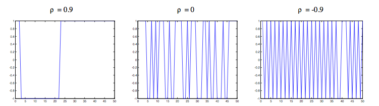
Figure 1. Simulation of the Markov Chain At under ρ = 0.9, ρ = 0, ρ = -0.9 It is straightforward to see how the behaviour of these processes meets the features outlined above in terms of persistency. Since the persistency of the additionality/crowding-out effect of subsidy on firm R&D is a central issue, the paper aims at comparing the model's outcomes under different degrees of persistency (i.e. different level of ρ ). In particular we want to see how subsidy inefficient provision could depend crucially on ρ .
- 3.24
- But to what extent is the level of "persistency" linked to the agency "selection process" adopted for choosing financeable R&D projects/firms? What can be approximately assumed is that when the persistency is very low (for example, ρ = -0.9) the agency is expected to have chosen firms/projects to finance with the aim of generating a continuous replacement. For example, the agency could have wanted to favour a wider access to funds inter-temporally by changing continuously the beneficiaries without taking into account what results have been reached in the past. On the contrary, when the persistency is higher and in particular when ρ is equal to zero, the agency might be thought of as selecting firms at random: the probability of staying in the same state and that of changing state is, in this case, exactly the same. When, finally, ρ is positive and close to one, then the agency appears to have given special importance to past selection choices, thus generating a perpetuation phenomenon favouring probably the same beneficiaries. In short: (i) continuous replacement, (ii) random assignment and (iii) perpetuation in selection, seem to be three potential situations whose differential effects are worth assessing.
The logic of the model
- 4.1
- Why should, in our model, the strategic agency-firm interplay generate a suboptimal provision of R&D subsidies? To better answer this question it seems useful to look at the objective function of both the agents involved in the game when, for instance, At is equal to 1. In this case the agency payoff increases monotonically as soon as r increases. It means that any higher level of r is strictly preferred to any lower level. By contrast, when s increases it first generates increasing utility and, after a certain threshold, a decreasing pattern. It depends on the balance constrain of the agency that does not have access to unlimited resources. As seen above, it leads to a quadratic form of the agency utility in s (inverted-U shape).
- 4.2
- The firms' profit behaves symmetrically. It increases monotonically as soon as s increases. It means that any higher level of s is strictly preferred to any lower level. By contrast, when r increases it first generates increasing utility and, after a certain threshold, a decreasing pattern since doing r is not costless and a financial constraint, beyond a certain threshold, does hold.
- 4.3
- Since we are supposing that agency and firms play a simultaneous game and given the forgone conditions, it is quite easy to show that the "rival" model is characterized by a time moving Cournot-Nash equilibrium that generally is not an optimum according to the Paretian criterion. In order to show this result we present a pivotal Prisoner's Dilemma-type example using a simple representation of the game with given payoffs.
- 4.4
- We suppose that both r and s can assume just two values: high or low. Given the fact that the profit as well as the agency welfare are inverted-U shapes, during the simulation it could happen that on the part of the firm, sometimes a low r will be preferred to a high r and sometimes the opposite might occur. Similarly, on the part of the agency and according to the evolution of the model, sometimes a low s will be preferred to a high s and sometimes the opposite will occur. Generally, four cases could appear whatever s for the firm and r for the agency, that is:
Case 1. For the firm r low is preferred to r high; for the agency s low is preferred to s high;
Case 1. Table 1 sets out the form and solution of the game in case 1. Let's start with the agency strategy. Either by choosing a high level of s or a lower one, the agency always prefers a higher r. Indeed, when r is high and s is high too the agency gets a utility of 15 against a utility of 5 when r is low. When r is low performing a higher s is more expensive and the agency prefers a lower s (with a utility of 10 against 5). The payoff of the firm is symmetric. The firm prefers always a higher level of s. When r is high it gets a profit of 15 when s is high and 5 when s is low. Vice versa, when r is low. Under these assumptions it is easy to see that the equilibrium of the "rival" model is (r-low, s-low) while the cooperative solution, found by maximizing the sum of the two payoff, is (r-high; s-high) where this sum is 30 against 20 in the Nash solution.Case 2. For the firm r low is preferred to r high; for the agency s high is preferred to s low;
Case 3. For the firm r high is preferred to r low; for the agency s low is preferred to s high;
Case 4. For the firm r high is preferred to r low; for the agency s high is preferred to s low.
Case 2. The firm prefers r-low to r-high whatever s, but the agency prefers s-high to s-low. The game form is visible in table 2. It is straightforward to observe that the new equilibrium is (r-low; s-high), while the optimal value is again (r-high; s-high).Table 1: Game representation under Case 1 Agency s-high s-low Firm r-high 15;15 5;20* r-low 20*;5 10*;10*
Case 3. Table 3 shows the game outcome in case 3. For the firm now r-high is preferred to r-low whatever the level of s. But for the agency s-low remains preferred to s-high whatever the level of r. It is easy to see that the new Nash equilibrium is (r-high; s-low) while in (r-high; s-high) the sum of utilities is again greater.Table 2: Game representation under Case 2 Agency s-high s-low Firm r-high 15;20* 5;15* r-low 20*;10* 10*;5
Case 4. Whatever s, for the firm r-high is preferred to r-low and whatever r for the agency s-high is preferred to s-low. In this case the Nash equilibrium of the game is equal to the optimal one (r-high; s-high) .Table 3: Game representation under Case 3 Agency s-high s-low Firm r-high 20*;15 10*;20* r-low 15;5 5;10*
According to this example, it is quite easy to see how the externality generated by the rival strategic interaction leads to an underprovided level of both r and s, while cooperative behaviour always leads to an higher level of s and r. Cooperation "internalizes the externality generated by the firm-agency rival behaviour", inducing a better systemic performance (as it occurs in the case of a generic "positive externality").Table 4: Game representation under Case 4 Agency s-high s-low Firm r-high 20*;20* 10*;15 r-low 15;10* 5;5 - 4.5
- Observe that the Nash equilibrium of case 4 is optimal as it is equal to that reached by the cooperative behaviour. It means that—along the time pattern - the sum of the two agents' objective function under rivalry is always lower than the social welfare function under cooperation, although sometimes it could be equal. In other words, the cooperative equilibrium is an upper bound of the rival one. Similar conclusions can be found in the case in which At takes a negative (rather than a positive) value (-1), in what case the subsidy generates "negative" rather than "positive" externalities on firms' profit.
Simulation results
- 5.1
- In order to get simulation results from the model we need to parameterize the model, by choosing parameters' level and the starting point of our simulations. Parameters have been chosen to get reliable and coherent values of the variables considered (to avoid, for example, negative sign for variables that ought to be positive, and so on). Furthermore, as the "ratio of r to s" is the central variable of our analysis, we set to start our simulations at a level or r/s close to that found in real data (about 40%) as shown in table 5, where data are drawn from the Unicredit/Capitalia survey on Italian manufacturing firms in the period 1998-2001. Meaning and level of the various parameters are set out in table 6.
Table 5: Some sample descriptive statistics Number of observations 3,452 Share of total R&D expenditure by financial source (supported firms): Self-financing 53 % New equity 1 % Debt 6 % Subsidy 39 % Table 6: Meaning and values of parameters φ0 fi0 25 Scale parameter of the R&D Marginal Rate of Return (MRR) φ1 fi1 5 Slope parameter of the R&D Marginal Rate of Return (MRR) μ mu 1.5 Fixed cost parameter of the R&D Marginal Capital Costs (MCC) β beta 8 Subsidy effect parameter of R&D Marginal Capital Costs (MCC) γ gamma 1 Knowledge stock effect parameter of R&D Marginal Capital Costs (MCC) δ delta 0.15 Depreciation rate of knowledge stock ψ psi 20 Parameter governing the cost of providing subsidies for the agency β0 beta0 0.96 Agency inter-temporal discount rate ρ rho -0.9, -0.5, 0, 0.5, 0.9 Persistency parameter (ranging between -1 and 1) - 5.2
- Figure 2 sets out our model's simulation results obtained by comparing rival and cooperative outcomes of a simulation with 10,000 replications with a ρ set up equal to 0.5 over a time span of 50 periods. The observed patterns are average values over these 10,000 runs.
Figure 2. Model Simulations with ρ = 0.5 - 5.3
- This simulation of the model shows very interesting results. First, both the level of R&D expenditure and subsidy is found to be severely undersized, as in the rival case they both are lower than in the cooperative case. It emphasizes not only that the subsidy is unable to generate the optimal level of R&D, but that this phenomenon is due primarily to the fact that the level of the subsidy provided by the agency is too much low compared to the socially optimal amount. Consequently, the ratio s/r is undersized as the optimal average level over the 50 periods simulation should be (on average) about 50% while it is only about 40% in the rival case: it means that the agency should provide about a 23% higher level of the s/r ratio currently provided if it wants to achieve the social optimum. This is the main policy consideration offered by this model. The results on the agents' payoffs are also worth to stress: rival situations tend to advantage more the agency than the firm, and the optimal level reached by cooperation tends to reduce the payoff of the agency in favour of firm profits. Also in terms of overall welfare, as expected, results show the dominance of the cooperative outcome over the rival one. In what follows we sum up these findings:
- 5.4
- Conclusion 1. The relative quota of s to r (i.e., the ratio s/r) is undersized in the rival compared to the cooperative model. It means that an increasing level of s/r is needed to reach welfare-superior results.
- 5.5
- Conclusion 2. The rivalry strategy generates distortions that favour the agency compared to firms. This distortion can be healed by an increasing s/r ratio.
- 5.6
- Let us now turn to the results under different path-dependence assumptions. Table 7 reports the results for five levels of ρ (-0.9, -0.5, 0, 0.5, 0.9) on various model endogenous variables. The values reported in this table are interpreted as "distortions" (or "biases") of the rival outcome when compared to the Pareto-efficient benchmark, that is:
100(Yc-Yr)/Yr where Yc is the cooperative outcome on variable Y and Yr the generic rival outcome.
- 5.7
- Generally speaking, the 50 periods simulations put into evidence a quite clear regularity: as long as we pass from a very low persistency of At (-0.9) to the highest one (+0.9) we get an increasing level of the "rival inefficiency" (or "welfare-bias") in terms of s, r and s/r, but with a parallel increase of the variance of results over the 10,000 replications considered. For example: the s/r ratio bias when ρ is equal to -0.9 is about 4.6% that is substantially lower than that of 32.6% reached when ρ is equal to 0.9; nevertheless, the coefficient of variation in the latter case (1,309) is about seven time greater than in the former case (194). It means that when the persistency of the additionality/crowding-out effect is weaker (stronger), the potential welfare-bias is lower (higher), but with a variance that is generally higher (lower). It means that a sort of trade-off between the reduction of the bias and the level of variance (risk) when moving from a lower to a higher persistency does arise. Similar results can be drawn by looking at what happens in terms of the level of s and r. Overall, it leads to the following conclusion:
- 5.8
- Conclusion 3. In passing from less persistent to more persistent R&D additionality/crowding-out effect, the lower the bias the greater the variance is and vice versa, so that a dominant choice of ρ does not emerge.
NOTE: CV = |St. Err./Mean*100|. Reference variable: 100*(Yc - Yr)/Yr where Yc = cooperative outcome, Yr = rival outcome. ρ = degree of persistency in additionality/crowding-out effect.Table 7: Simulation results of model endogenous variable under different levels of ρ 1 2 3 4 5 6 7 8 9 Subsidy Stock
of knowledgeMarginal
capital
costs
(MCC)Marginal
rate of
return
(MRR)Agency profit Firm profit Ratio
s/rR&D expenditure Welfare Mean ρ = -0.9 Mean 12.36 3.21 -5.61 -2.07 -98.90 2.52 4.61 3.36 0.64 -8.88 St. Err. 72.60 0.87 9.56 1.13 323.54 4.58 60.31 1.88 7.03 53.50 CV 587.40 27.08 170.37 54.76 327.13 181.92 1309.69 56.12 1104.75 424.36 ρ = -0.5 Mean 8.22 1.89 -4.67 -1.25 -24.77 1.89 4.02 2.01 0.43 -1.36 St. Err. 22.43 0.51 4.87 0.70 133.16 2.45 18.46 1.25 1.16 20.55 CV 272.99 26.69 104.14 55.95 537.48 129.36 459.53 62.43 273.17 213.53 ρ = 0 Mean 58.21 1.98 -14.17 -1.44 -236.63 5.18 34.83 2.26 2.54 -16.36 St. Err. 68.96 0.79 8.87 0.57 3661.68 3.02 24.50 0.89 2.05 419.04 CV 118.46 40.01 62.58 39.36 1547.41 58.39 70.35 39.21 80.63 228.49 ρ = 0.5 Mean 27.08 1.64 -9.99 -1.17 -151.98 3.65 22.98 1.82 1.51 -11.61 St. Err. 14.33 0.60 4.47 0.39 119.27 1.54 13.35 0.61 1.13 17.30 CV 52.92 36.35 44.76 33.14 78.48 42.13 58.10 33.52 74.70 50.46 ρ = 0.9 Mean 39.73 2.15 -10.83 -1.49 -62.55 4.19 32.57 2.33 1.69 0.86 St. Err. 75.44 0.77 6.44 0.99 151.19 3.51 63.18 1.66 2.28 33.94 CV 189.89 35.67 59.46 66.42 241.70 83.79 193.98 71.33 135.42 119.74 As for the alleged optimal level of ρ , the only aspect that can be stressed is the good compromise represented by the case in which of ρ is equal to 0.5, where the welfare-bias is not too harsh and the variance is at the same time quite small.
- 5.9
- What policy message can we draw from this analysis? Of course there is not a "direct" mechanism to control the level of persistency of the additionality/crowding-out effect. In this sense there is not a specific policy instrument on the part of the government. What less ambitiously our results aim at suggesting is to take this "persistency behaviour" as a sort of "cautionary note" when providing R&D subsidies to private corporations via public agencies. Of course, the "selection into the R&D supporting program" mechanism can roughly give some direction to the process, although limited and approximated. In this sense, a selection mechanism aimed at awarding quite recurrently the same subjects could probably encourage some persistency thus producing an increasing likelihood of stronger biases; but also a continuous replacement, although promoting a little less persistency, has its drawback as it renders - on average - the outcomes less biased even though with a very higher level of results' variability. Our model seems to suggest to be not too much extreme in positioning the selection mechanism between perpetuation on the one hand and continuous replacement on the other, as both seem to engender problems. It goes without saying that these results also depend crucially on the "quality" (i.e., degree of success/failure) of firm R&D projects that, together with the selection mechanism, drives the realization of At; it is for this reason that our conclusions have to be taken only as indicative suggestions and not as prescriptive policy recommendations.
Conclusion
- 6.1
- The simulation model presented in this paper shows quite clearly to which extent the level of R&D subsidies chosen by an inter-temporal maximising funding agency could be severely undersized. This is the main result of the time-moving Cournot-Nash equilibrium generated by the agency-firm game. The model predicts under this assumption that both private R&D and R&D support are too low compared to the social optimum, thus generating a "policy failure" that previous studies dealing with this subject seemed to have somewhat overlooked.
- 6.2
- As for more detailed results, after running 10,000 simulations of the rival and cooperative model under a "medium" level of persistency (ρ = 0.5) over 50 periods we get that, on average, the "rival" strategy sets out a subsidy-R&D ratio about 10% lower than the "cooperative" (that is, the "optimal") one: the share of R&D subsidy on total R&D proves thus to be undersized with respect to its optimal level. This result is confirmed along various values assumed by the persistency parameter of the Markov Chain. Interestingly, we also find that the "welfare distortions" due to strategic interaction are lower when persistency is lower and vice versa, although the variability of this result is higher in the case of low persistency than in the opposite case. It means that a public actor who wants to reduce welfare distortions has to cope with a sort of trade-off between the degree of distortion and its variability. In this sense, according to our results, a dominant level of the persistency parameter does not arise.
- 6.3
- According to our findings two issues seem to be important for the management of R&D funding policies: (i) all the elements favouring greater cohesion and collaboration between agency and firm objectives (i.e., less rival policy settings) can help to move the level of current R&D support towards its social optimum[2]; (ii) the selection mechanism operated by the public agency, needs to be not too much extreme between perpetuation (when awarding the same subjects over time) on the one hand and continuous replacement (when changing financed firms continuously) on the other, as both seem to generated suboptimal situations.
Appendix A: Structure of the simulation program
- A.1
- This appendix provides a brief "read-me" for the basic file used to perform the simulations carried out in the paper. The Matlab M-file "RD_policy_duopoly_and_sp_stochastic.m" is the main simulation code. It contains all the needed code, while the only external function called by this program is the function "simulate_markov2.m" used for generating the Markov Chain of At. The basic structure of this file is the following:
1. INITIALIZATIONS 1.1 Initialize the simulations (i.e., the matrices for the variables) 1.2 Set parameters for the Bellman equation 1.3 Set parameters for the first-order Markov process of A=theta For the "Duopoly" first and then for the "Social-planner" objective function: 2. VALUE FUNCTION ITERATION (for finding the "optimal policy function") 2.1 Set state-space 2.2 Calculate the "policy function" of the Bellman equation (i.e., the solution of the stochastic dynamic optimization problem) by "value function iteration" 2.3 Generate the "policy function" and graph it 3. SIMULATION 3.1 Simulate the Markov Chain of A=theta 3.2 Set the vector for the simulated time-series of the variables 3.3 Choose initial values for the R&D capital and then simulate the temporal movement of all the variables Both for the "Duopoly" and the "Social-planner": 3.4 Calculate variables' average over the M = 10,000 simulations to get the average temporal patter. - A.2
- Observe that with the term "Duopoly" we intend here the "non-cooperative" (or "rival") strategy as defined in the paper, as well as with "Social-planner" we mean the cooperative (or Pareto-efficient) solution of the model. Observe that within this program the Markov Chain of At is called "theta" (instead of A). At heart of the procedure contained in "RD_policy_duopoly_and_sp_stochastic.m", there is the code for calculating the "optimal policy function", i.e., the solution of the inter-temporal maximization problems expressed by formulas (4) and (5) in the paper. We chose to use the method of "value function iteration" and the main reference for this program is the book by Miranda and Fackler (2002).
Notes
-
1There is a huge theoretical and empirical literature on the determinants of firm RDI behaviour. See, for instance: Mansfield (1964), Nadiri (1979), Cohen and Levinthal (1990), David and Hall (2000). The DHT model, in particular, assumes that the R&D's MRR depend on: technological opportunities, state of demand, appropriability conditions; and that the R&D's MCC depend on: technological policy tools, macroeconomic conditions, external costs of funds, venture capital availability. Compared to this approach, the model proposed in this paper is a very schematic and simplified representation of firm R&D choice, allowing for fewer determinants. Beyond the need of a better analytical tractability of the model, this choice reflects the aim of focusing primarily on the relation between the endogenous determination of firm R&D and that of public subsidization, by taking all the remaining exogenous determinants as ceteris paribus conditions.
2As widely recognized, for example, a larger firm project information disclosure could be a good strategy for promoting greater cooperation, as well as better comunication and agreement between the public agency and the firm on sharing and exploiting project outcomes.
References
-
ALCHIAN A A and Demsetz H (1972). Production, Information Costs, and Economic Organization. The American Economic Review, 62, pp. 777-795.
ARROW K (1962) Economic Welfare and the Allocation of Resources for Invention. In Nelson R (Ed.), The Rate and Direction of Economic Activity, Princeton University Press, New York, pp. 609-25.
BENTAL B and Peled B (2002) Quantitative Growth Effects of Subsidies in a Search Theoretic R&D Model. Journal of Evolutionary Economics, 12, pp. 397-423. [doi:10.1007/s00191-002-0125-9]
BERLE A A and Means G C (1932) The Modern Corporation and Private Property, Brace & World, New York: Harcourt.
CERULLI G and Potì B (2012), The differential impact of privately and publicly funded R&D on R&D investment and innovation: the Italian case. Prometheus. Critical Studies in Innovation, forthcoming. [doi:10.1080/08109028.2012.671288]
COHEN W M and Levinthal D A (1990) Absorptive Capacity: A New Perspective on Learning and Innovation. Administrative Science Quarterly, 35, pp. 128-152. [doi:10.2307/2393553]
DAVID P A and Hall B H (2000) Heart of Darkness: Modeling Public-Private Funding Interactions inside the R&D Black Box. Research Policy, 29, pp. 1165-1183. [doi:10.1016/S0048-7333(00)00085-8]
DAVID P A, Hall B H and Toole A A (2000) Is Public R&D a Complement or Substitute for Private R&D? A Review of the Econometric Evidence. Research Policy, 29, pp. 497-529. [doi:10.1016/S0048-7333(99)00087-6]
DAVIDSON J and De Jong R (1997) Strong laws of large numbers for dependent heterogeneous processes: a synthesis of recent and new results. Econometric Reviews, 16, pp. 251-279. [doi:10.1080/07474939708800387]
DASGUPTA P and Stiglitz J (1980) Industrial Structure and the Nature of Innovative Activity. The Economic Journal, 90, pp. 266-293. [doi:10.2307/2231788]
DASGUPTA P (1988) Patents, Priority and Imitation or, the Economics of Races and Waiting Games. The Economic Journal, 98, pp. 66-80. [doi:10.2307/2233511]
D'ASPREMONT C and Jacquemin A (1988) Cooperative and Noncooperative R&D in Duopoly with Spillovers. The American Economic Review, 78, pp. 1133-1137.
ERICSON R and Pakes A (1995) Markov-Perfect Industry Dynamics: A Framework for Empirical Work. Review of Economic Studies, 62, pp. 53-82. [doi:10.2307/2297841]
HALL B H (2002) The Financing of Research and Development. Oxford Review of Economic Policy, 18, pp. 35-51. [doi:10.1093/oxrep/18.1.35]
HOWE J D and McFetridge D G (1976) The Determinants of R&D Expenditures. Canadian Journal of Economics, 9, pp. 57-71. [doi:10.2307/134415]
LAINCZ C A (2009) R&D subsidies in a model of growth with dynamic market structure. Journal of Evolutionary Economics, 19, 5, pp. 643-673. [doi:10.1007/s00191-008-0114-8]
JOU J and Lee T (2001) R&D investment decision and optimal subsidy. R&D Management, 31, pp. 137-148. [doi:10.1111/1467-9310.00204]
MALERBA F (1993) The National System of Innovation: Italy. In Nelson R (Ed.), National Innovation Systems. A comparative Analysis. Oxford University Press, Oxford, pp. 230-60.
MANSFIELD E (1964) Industrial Research and Development Expenditures: Determinants, Prospects, and Relation to Size of Firm and Inventive Output. Journal of Political Economy, 72, pp. 319-340. [doi:10.1086/258914]
MARTIN S and Scott J T (2000) The Nature of Innovation Market Failure and the Design of Public Support for Private Innovation. Research Policy, 29, pp. 437-447. [doi:10.1016/S0048-7333(99)00084-0]
METCALFE S (1995) The Economic Foundations of Technology Policy: Equilibrium and Evolutionary Perspectives. In Stoneman P (Ed.), Handbook of the Economics of Innovation and Technological Change. Blackwell Publishers, Oxford, pp. 409-512.
MATERIA V C and Esposti R (2009), Modelling Public R&D Cofinancing within a Principal-Agent Framework. The Case of an Italian Region, paper presented at the "50a riunione scientifica annuale Società Italiana degli Economisti".
MIRANDA M J and Fackler P L (2002), Applied Computational Economics and Finance. The MIT Press.
MOWERY D (1995) The Practice of Technological Policy. In Stoneman P (Ed.) Handbook of the Economics of Innovation and Technological Change. Blackwell Publishers, Oxford, pp. 213-557.
NADIRI M I (1979) Contributions and Determinants of Research and Development Expenditures in the U.S. Manufacturing Industries. NBER Working Papers, No. w0360.
POTÍ B and Cerulli G (2011) Evaluation of firm R&D and innovation support: new indicators and the ex-ante prediction of ex-post additionality. Research Evaluation, 20, pp. 19-29. [doi:10.3152/095820211X12941371876427]
VARIAN H R (1992). Microeconomic Analysis, New York, W.W. Norton.
WILLIAMSON O E (1964) The Economics of Discretionary Behaviour: Managerial Objectives in a Theory of the Firm. Englewood Cliffs, NJ: Prentice-Hall.