
 Abstract
- In this study we describe a simulation platform used to create a virtual society of Poland, with a particular emphasis on contact patterns arising from daily commuting to schools or workplaces. In order to reproduce the map of contacts, we are using a geo-referenced Agent Based Model. Within this framework, we propose a set of different stochastic algorithms, utilizing available aggregated census data. Based on this model system, we present selected statistical analysis, such as the accessibility of schools or the location of rescue service units. This platform will serve as a base for further large scale epidemiological and transportation simulation studies. However, the first approach to a simple, country-wide transportation model is also presented here. The application scope of the platform extends beyond the simulations of epidemic or transportation, and pertains to any situation where there are no easily available means, other than computer simulations, to conduct large scale investigations of complex population dynamics.
- Keywords:
- Agent Based Model, Educational Availability, Daily Commuting, Social Network, Virtual Society Simulations
Introduction
- 1.1
-
The threats posed by highly pathogenic respiratory diseases, like SARS, current spread of the novel, swine-like influenza A/H1N1 virus, or the eventual spread of avian flu virus, require health authorities to prepare for the possibility of a human pandemic. Especially, some control strategies need to be planned, and should they be deemed effective, implemented. School closure is among the measures most often considered. In the recent studies (Cauchemez et al 2008), the effect of such closure on influenza epidemic spread was estimated with the usage of Monte-Carlo stochastic simulation method. Previous models were dealing with the simulations of influenza spread in Thailand (Ferguson et al 2005), or in the UK and US (Ferguson et al 2006). In each case an individual-based simulation model was used to parametrize either a pandemic influenza transmission (Ferguson et al 2003), or a spread of the foot and mouth disease in the UK (Ferguson et al 2001). A similar approach was also used to study influenza spread in the USA (Germann et al 2006), implementing a very large-scale simulation involving over 200 million of geo-referenced software agents, using statistical models, or implementing a smaller scale model of epidemics spread in southern California, USA (Stroud et al 2007). In both independent USA studies (Ferguson et al 2006; Germann et al 2006) their findings were in good qualitative agreement, enhancing each other, but most importantly demonstrating the practical usefulness of very large-scale simulations. Another example of the platform for general purpose epidemics simulation is MASON (Dunham 2005).
- 1.2
-
Applications of large-scale Monte Carlo type simulations aimed at mimicking a social context are not, of course, limited to the epidemiology alone. Ever since its inception over two decades ago (Galam 2004; Pabjan 2004) the interest in sociophysics, especially in modeling social dynamics (Bertotti and Delitala 2006,Ballas et al 2007) has grown considerably, spawning numerous sub-fields and their variants. Besides the epidemiology, macro-economical studies (Bai et al 2008) and supply-chain operational research (Hammami et al 2008), two other areas share the requirement and the need for large scale simulations, namely, transportation systems and ecology (Beckmann et al 1996; Granger 2001; Hogeweg 2007).
In particular, sustainable transport systems (Richardson 2005), transportation induced CO2 emissions in the USA (Lakshmanan and Han 1997), air transport systems (Janic 2000), and modeling alternatives between quick, intercity railroad and air networks (Kutakh and Fursova 2003; Svenson et al 2006), or transportation decision support systems for the whole of Turkey (Ulengin et al 2007) can serve as a good introduction. Distinct transportation problems arise in the urban context, where, e.g., the probability of congestion and traffic jams is particularly high. Rickert and Nagel introduced an ABM system (which they dubbed a micro-simulation model) called TRANSIMS to deal with issues of this kind (Rickert and Nagel 2001;Cetin et al 2002) and even proposed to extend their solution to the whole of Switzerland (Raney et al 2002). - 1.3
-
Agent based models (ABMs) are devised to describe explicitly the interactions among individuals and their environment, thus providing a process-oriented alternative to strictly analytical mathematical models (Goldstone and Janssen 2005). The construction of such models requires, however, a generation of the system of the, so called, software agents, as well as the geo-referenced network of public objects (like schools, factories, offices, hospitals, transportation systems, etc.), as well as with the selected elements of infrastructure. Due to high dimensionality of this virtual society (multiple agents operating on multiple contexts), the evolution of such system is typically performed using the stochastic Monte-Carlo methods. Moreover, sometimes even the preliminary creation of such complex system, mostly because of the scarcity of the real data, calls for the usage of stochastic methods.
The issues involved in the construction of virtual society stem mostly from a need to recreate details of the information contained, usually buried in aggregated data as delivered by national census bureaus, and/or other such services. There is a need, then, to devise techniques allowing for either deconvolution of various sources of the aggregated data into their constituting components, or reconstruction of original data, by building geo-referenced software constructs, which can serve as a reasonable approximation of the missing data with detailed enough granulation (see Ferguson et al 2003; Ferguson et al 2005; Ferguson et al 2001) for the examples of approaches geared for the reconstruction of the educational system in Thailand or Birkin et al 2006 for the thorough reconstruction of the UK population). - 1.4
-
This work aims at the development of methods used for construction of the virtual, agent based model of local population densities, educational and workforce networks, and social interactions combined together to produce the social fabric of 38 million agents. This will serve as the basis for subsequent epidemiological and transportation studies. As an example of application of the AB system constructed here, the simple analysis of the school accessibility in Malopolskie voivodeship was performed, namely, the results obtained within the model described here were collated with (unfortunately, the only available at the time of this study) statistical data. Although the quantitative calibration was not possible, qualitative correlation turned out to be noticeable. Another use of the model is a simplified analysis of the number and locations of rescue service units (RSUs) in local communes. Although it certainly requires a significant development, the model opens the way to a country-wide, immediate analysis of the effectiveness of possible location of RSUs.
- 1.5
- The structure of this work is the following: Section 2 briefly describes the statistical data sources, and gives basic statistical information with regard to Poland. In Section 3 the methodology used to create the virtual Polish society is described, and Section 4 presents the resulting virtual society, together with the analysis of both the schools' accessibility, and the simplified, tentative RSUs' localization.
Data
- 2.1
-
Population data accessible for Poland comes from the two sources: the LandScan, and Polish Regional Data Bank (BDR) maintained by National Census Bureau (NCB).
The LandScan service delivers data of an instantaneous population density with a resolution of 1 km. The output map, covering the entire globe, is based on the data and their statistical analysis reported by national census offices, remote sensing data analysis, terrain type analysis, ongoing agriculture studies, etc. It is an ASCII data file containing a rectangular matrix of the population in each node of the grid. In the present studies we were using the population density data from LandScan as released for the year 2004.
On the other hand, the NCB applies its own methods to perform the appropriate surveys and the aggregation of the data. In the end, the officially released data are limited to some extent by the local law regulations. Most of the data used in this work were obtained from the NCB Regional Data Bank, and some of them were taken from the annual NCB reports. Basic population statistics for Poland are given in Table 1.
Table 1: Basic population and infrastructure statistics for Poland. Population 38.2 million Women 19.7 million Households 13.3 million Men 18.5 million Primary school pupils 2.9 million Primary schools 13.7 thousand Secondary school pupils 1.6 million Secondary schools 6.3 thousand College students 1.4 million Colleges 1.9 thousand Employees 7.7 million Workplaces 140 thousand - 2.2
-
Any data coming from Polish NCB are given within the Polish administrative system framework. A basic administrative unit in Poland (equivalent to a borough or a county) is called a commune. Following the European Nomenclature of Territorial Units for Statistics (NUTS) it is classified as NUTS-1. There are three types of such units: a rural commune, which comprises a territory of several villages, a urban-rural commune - as the latter, but with a dominant small city, and a urban-commune - the territory of a large city. The areas of such communes vary substantially, from 2 up to 664 square kilometers. More details regarding commune types such as their cumulative area or the cumulative population in each commune type are given in Table 2. An administrative unit superior to a commune and composed of several of them, is a poviat (NUTS-4). There are 2490 communes and 379 poviats in Poland. At the highest level of this administrative hierarchy is a voivodeship (NUTS-2), which divides Poland into 16 units. The map of voivodeships is shown in Figure 1 and some more statistical details for two voivodeships are given in Table 3.
Table 2: Basic administrative statistics for Poland. Commune type Number Total area [km2] (%) Population (%) Urban 318 15.4⋅103 (4.9) 20.4 ⋅106 (53.7) Rural 1589 199 ⋅103 (63.4) 9.7 ⋅106 (25.6) Urban-rural 583 99.5⋅103 (31.7) 7.9 ⋅106 (20.7) Total 2490 314⋅103 38 ⋅106 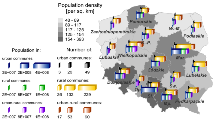
Figure 1: Statistics for Polish voivodeships. In stacked-bar representations: the number of communes for each commune type and the population in each commune type. Within each representation bars are drawn in a common scale. In hatch-map representation: the population density in voivodeships. Abbreviated voivodeship names stand for: Warminsko-Mazurskie (W-M), Kujawsko-Pomorskie (K-P), Mazowieckie (Maz), Opolskie (Op), Swietokrzyskie (Sw), Slaskie (Sl), Malopolskie (Mp). - 2.3
-
Two voivodeships are presented in Table 3, namely, Mazowieckie and Slaskie, as the most interesting and quite different examples. Mazowieckie voivodeship is the one with a capital city and Slaskie is basically the largest industrial region in Poland. They are the mostly populated voivodeships (each contains 13% of the population and around 50 urban communes, that is cities). However, in terms of area, while Mazowieckie voivodeship is the largest one, Slaskie is one of the smallest. One can see, that Slaskie is covered by urban areas quite significantly (in 25%). Thus, the population of Slaskie voivodeship is quite densely and uniformly spread around the entire area, while most of the Mazowieckie population resides in the capital city, and the remaining area of the voivodeship is covered by rural communes.
Table 3: Administrative statistics for two Polish voivodeships Voivodeship Number of communes:
urban/rural/urban-ruralPercent of voiv. area:
urban/rural/urban-rural communes
(% of total area)Percent of voiv. population:
urban/rural/urban-rural communes
(% of total population)Mazowieckie 46 / 229 / 50 5 / 76 / 19 (11) 58 / 27 / 15 (13) Slaskie 49 / 96 / 22 26 / 55 / 19 (4) 84 / 9 / 6 (13) - 2.4
- Statistical data from NCB were acquired from Polish NCB server using bash scripts managing perl scripts. The latter implemented the HTTP::Request::Common constructor of HTTP::Request objects, HTTP::Cookies, and LWP::UserAgent classes. Separate scripts were used for each type of data (population, education or employment statistics). On the output of the above scripts there were ASCII data files containing the desired data.
Methods and techniques
- 3.1
-
The information obtained from LandScan and NCB constituted the input data for socstr program, written in C++, that was used to create Polish virtual society reported here. A schematic workflow used to generate this virtual society is presented in Figure 2. A detailed description is given in the figure caption. Any output from socstr, either an intermediate or a final file (any of the green rectangles surrounded by solid line in Figure 2), contained list of data. E.g. Basic Virtual Society is a list of households' id numbers with their coordinates, with the number of agents they hold, and with the id numbers of these agents.
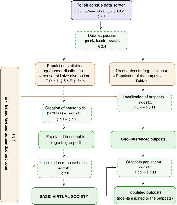
Figure 2: The workflow used to generate the virtual society reported in this work. Diagram fields are color coded: blue corresponds to on-line data server, brown designates data files obtained from data servers (LandScan or NCB). Green rectangles drawn with a solid line mark data files created by socstr program, green rectangles drawn with a dashed line correspond to numerical procedures. Dashed arrows are used just to mark, that one can run socstr to create the basic virtual society and then add any outposts or one can use the basic virtual society created at the beginning as an input to socstr only to add any outposts.
Basic virtual society
- 3.2
-
We define here a basic virtual society (BVS) as a set of populated and geo-referenced (located) households. Populated means that the whole virtual (software) population is spread among virtual (software) households. Moreover, it is spread according to the age and gender distributions in each voivodeship (data obtained from NCB). In other words, every individual from the population, described by its age and gender, is assigned to a particular household. Also, each household in the BVS has a geographic location assigned to it, or in other words, it is located. Data obtained from the NCB, namely, the age and gender distributions and the household size distribution, are aggregated up to the level of voivodeships. Hence, urban or rural demographic variation is not strictly taken into account. Namely, structure of a household does not depend on its administrative location (urban or rural one), although e.g. one should expect larger families in rural regions.
However, households are located on the basis of the second data source - the LandScan population density, which provides data with 1 km resolution. This allows to reproduce the population density structure/variability even across the commune.
Populating the households
- 3.3
-
The age and gender distribution in a real household is obviously not random, so the structure of a virtual household should also reflect some possible relationships, such as those of mother and child, or wife and husband. Hence, in order to reproduce realistic populations within households, a stochastic algorithm is proposed allowing for the agents' assignment to households.
- 3.4
-
First, the whole set of households was divided into 16 subsets, where the distribution of subsets' sizes matched exactly the distribution of the households' number in Polish voivodeships taken from the NCB. Subsequently, within each virtual voivodeship, the households' sizes were established in exact accordance with the households' size distribution within corresponding voivodeship taken from the NCB.
- 3.5
-
In order to assign a software agent (of a given age and gender) to a given household, the following rules were devised:
- Children (age 0-24) and parents were treated separately.
- Children were not placed in empty households.
- For each member in the household, the probability of attraction (denoted as pa) or competition (pc) between given member and the agent to be assigned were calculated. The probabilities, shown in Figure 3, were chosen arbitrarily, and were dependent only on the age difference, τ, between a given household-member and the agent to be placed. To give an example, a child-aged agent was placed in a household only if there was already a parent-agent in this household, and only if this agent was old enough to be a parent of this particular child to be placed. There were 3 kinds of attraction probabilities, and one competition probability:
- the probability of the attraction between a child-age agent and an adult female agent, pa(τchild-female),
where τchild-female = agefemale - agechild;
It was set to zero for the age difference less than 15 (to allow for the generation gap, that is, to ensure that mother is at least 15 years old). The highest pa value was set for the τchild-female = 26, with accordance to the census data (i.e. to the most frequent age among parturient women in Poland in 2002). - the probability of the attraction between a child-age agent and an adult male agent, pa(τchild-male),
where τchild-male = agemale - agechild;
It was set to zero for the age difference less than 18. - the probability of the attraction between an adult female agent and an adult male agent, pa(τfemale-male),
where τfemale-male = agemale - agefemale; - the probability of the competition between adults of the same gender, pc(|τss|), where |τss| is the absolute age difference between the agent to be assigned and a given household member of the same gender; Only the maximum pa and pc from all obtained within a given household were used in further calculations. The profiles of the pa and pc functions refer to the statistical distributions of the age difference between household members (mother and child or between spouses), they are not, however, exact distributions. The objective of the procedure described here is to establish reasonable sets of household members (families), and to eliminate those unfeasible, e.g. three member family with 2 males aged 1 and 3 years, and one female aged 2.
- the probability of the attraction between a child-age agent and an adult female agent, pa(τchild-female),
- The probability of the assignment of an adult agent in an empty household equals 1.
- The overall probability for a given agent's assignment in a given household was calculated using the following formula,
p = max{0; min{1; α + βpa - γpc}} , (1)
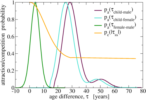
Figure 3: Probabilities used to create (populate) households. Location of households
- 3.6
-
In order to locate the virtual households the following algorithm, based on the LandScan population density map, was applied: the number of inhabitants in each node of the LandScan map constituted this node's threshold value for the virtual population being located. Each node was filled with households' members by a random choice of a virtual household from the voivodeship subset of virtual households. Every time, all members of the chosen household were added to the node. This continued while the total population in the node was still below the threshold value from the LandScan map.
Development of the BVS - schools and workplaces
- 3.7
-
Once the basic virtual society is created, every additional infrastructure network is developed using the same general workflow (right branch of the workflow depicted in Figure 2). First, specific outposts (any of the school types or workplaces) were located, then agents were assigned to the outposts. A detailed description of the methods used within the workflow is given in the following sections.
- 3.8
-
Typically, if the statistical data on geo-location and size of schools or workplaces are available, the so called gravity models are used (Ferguson et al 2006; Stroud et al 2007) to assign agents to the outposts. Otherwise, if the available or used data constrains only the total number of schools, workplaces (which is the case in this work) or the average school size, heuristic free-selection algorithms are implemented, e.g. allowing for a random selection of a school for each child under certain (mostly distance-dependent) constraints (Ferguson et al 2005;Ferguson et al 2006; Germann et al 2006). In our studies, the following methods were used to assign agents to primary and secondary schools, colleges, and workplaces.
- 3.9
-
Primary and secondary schools - Primary and secondary education levels, reserved for children 7-12 and 13-15 years old, respectively, are compulsory in Poland, thus schools at these levels are quite abundant in Poland (see Table 1). In order to locate these types of schools, the LandScan density map was used as a weight matrix for a stochastic distribution. Namely, the higher the population density in a given LandScan node, the higher the probability to locate a school there. The total number of schools in each commune was taken from the NCB. There was no information on the size of schools in the NCB. An agent of a primary (or secondary) school age was assigned to a randomly selected primary (or secondary) school located within 7 km radius from the location of the agents' household. If there was no school within such a radius, the agent was assigned to the nearest primary (or secondary) school located beyond that radius.
- 3.10
-
Colleges - There are significantly less colleges than lower level schools (see Table 1) in Poland because education on the college level is not compulsory. Consequently, there are communes without any college. Thus the poviat region was selected as a basic regional unit. As in the previous case, colleges were located based on the LandScan density map (serving as a weight matrix for a stochastic distribution within poviat). The total number of schools in each poviat was taken from the NCB. Also in this case there was no information on the size of colleges.
First, in order to introduce agents to virtual colleges, each college was populated by 2/3 with college-aged agents from its surrounding area of 30km radius. Then, the rest 1/3 of the college-aged agents from this area were assigned to the nearest college within their poviat.
One should note, that the LandScan data refer to the actual population density data, so e.g. LandScan considers pupils living in dormitories, whereas in the NCB database used here each pupil belongs to a certain virtual household.
- 3.11
-
Workplaces - The number of workplaces (see Table 1) and the size distribution of workplaces in each voivodeship were obtained from the NCB. The maximum single workplace size in Poland is 2992, the average size of a workplace is about 10 individuals. Workplaces were located using a similar method as for the location of households or schools, that is with the location probability proportional to the population density at a given node in the LandScan map. One should note, that there are very few large industrial zones in Poland and a lot of factories are located within the living zones. Pure city zones occupied only by bureaus, offices, and malls are rather sparse in Poland, so also these smaller but more numerous workplaces are mixed homogeneously within the living areas.
The assignment of agents to virtual workplaces was stochastic, with the probability of the assignment of a given agent to a given workplace dependent on the distance from the workplace to the agents' household. The probability was taken from the normal distribution, centered at the location of the workplace and with the standard deviation proportional to the size of the workplace.
The discrepancy between the number of workplaces in a given region and the population there gives the natural effect of daily commuting to large agglomerations.Rescue service units
- 3.12
-
The location of Rescue Service Units (RSUs) does not pertain to the reconstruction of a real social topology process, but constitutes a starting point in the analysis of the relation between the locations of households, and the assumed topography of any rescue service systems. The RSUs are generalized and can be substituted by any type of rescue services such as voluntary fire brigades, medical services, or epidemiological stations.
The redistribution of the RSUs was performed for each commune separately. Starting from one RSU, gradually up to twenty RSUs were placed (or attempted to be placed) in each commune. The probability of the location of any subsequent RSU in a given node on the grid was scaled by the corresponding LandScan density value. Additionally, the procedure was under the constraints imposed on the minimal pairwise distance between RSUs, which was set to 2 km.
Because we are interested in the general properties of Polish communes topology network, the calculations were carried out for each commune, yielding a relation between the mean household-RSU distance and the number of located rescue units in every commune. This way, it is possible to determine an optimal saturation with rescue units, comparing the benefits and the costs of establishing and funding of a new unit.Model of a long distance travelling
- 3.13
-
Travelling agents - simple transportation model
To account for the travelling of agents in an extended and detailed manner, knowledge of the explicit road and rail networks, or at least any statistics on everyday commuting/traffic would be necessary but these data were unavailable. However, at this preliminary stage, taking into account future epidemiological applications of this model, only the number of contacts at each transit point and the identities of the contacting agents were considered. For this reason, in our model we are applying a simple transportation model that uses an approximate city network.
For each travelling agent during his travel, the number and identities of co-travellers were determined. Finally, instead of considering the exact travel path, only the intermediate breakpoints (transfer cities) between endpoints (the origin and the target cities) were considered. The travelling dynamics simulations were carried out with the simulation time-step set to 1 day.
Below we provide a more detailed description of the travelling module. - 3.14
-
Shortest routes via breakpoints
First, in the preliminary step, the ncit largest cities were found, and the whole country was divided into ncit sub-regions, that is, ncit conglomerations corresponding to the ncit cities (centres of conglomerations). Treating cities as nodes of a directed weighted graph, the shortest path between any two nodes of the graph was found using Dijkstra (Dijkstra 1959) algorithm, where the weight of the edge between two consecutive nodes composed of the Cartesian distance between the two cities and the reciprocal of the population in the ending node (this explains the directed character of the graph). This way, the shortest path was the one leading through the mostly populated areas. A highly populated area - a large city - encompasses many railway stations allowing for transfers.
As an output of the above procedure one has an ncit x ncit matrix S of neighbours, where the sij element of the matrix keeps the identity (id) of the consecutive city after the ith one on the shortest route from node i to node j. It thus gives an easy access to both: the ids and the number of connecting nodes (cities). In the simulation tests carried out at this stage, we used ncit=38 which is the number of the cities in Poland with population number higher than 5⋅105. This population number threshold is a simulation parameter defining the number of the cities, ncit. Thus, decreasing this threshold increases the number of the cities considered. The S matrix is created once, at the beginning of the simulation. - 3.15
-
Stochastic model of travelling
Step 1 - choice of travellers At each time step (1 day) of a simulation, in a series of independent Bernoulli trials, some agents acquire the status of a traveller, where the probability of becoming a traveller in one trial, ptr, is a simulation parameter. The trial is repeated over all agents. In this work, ptr was set to 0.5⋅10-3 in all simulations, which yields an expected number of approximately 1.8⋅104 new travellers each time step (that is each day).Step 2 - choice of start and end points Each traveller starts his journey in the centre of his conglomeration. The destination of his travel is randomly chosen from the distribution of all geo-locations of agents. This means, that the more agents reside in a certain geo-location, the higher is the probability of travelling there. In other words, densely populated areas, such as cities are favoured as travel destinations.
Step 3 - choice of transfer cities As soon as the start and the end points of each journey are chosen, the possible route can be easily looked-up in the S matrix. However, the number of transfer breakpoints is also subject to a random choice. More precisely, how far can a given group of co-travellers on a given route go directly (without any transfer points) during one day is joint with a random number taken from the cumulative distribution of the population in the consecutive connecting cities. Such an approach is used to mimic a typical journey, where the transfers take place in major cities rather than in small ones. Also, accounting for the population in the target city in the cumulative population distribution may favour the direct route, especially in the case where the target city is large (typically, in Poland, if one travels to e.g. the capital city, there is a high chance he may go directly; but if one travels to a much smaller city in the neighbourhood of the capital, he'll probably need to make a transfer in the capital).
Step 4 - choice of co-travellers At each starting and transfer city, co-travellers (that is travellers who are at a given point and who head towards the same target) are bundled up randomly. That is, the bundle size is a random number taken from the uniform probability distribution in the range [0;max_bundle_size]. Members of the bundles are also chosen randomly (from a uniform distribution) from the group of all possible co-travellers. max_bundle_size was set to 10 for all simulations.
Results and discussion
- 4.1
-
We are reporting here only selected properties of Basic Virtual Society described here. In such a system various ranges of a quantitative analysis can be considered. However, we focus here on the features essential for the ongoing epidemiological and transportation studies, as well as on the planned future investigations. Since the methods used for the recreation of given social contexts, e.g. schools and workplaces are in principle similar, we limit the description only to one selected type of network structure.
Basic Virtual Society - population and location of households
- 4.2
-
The structure of households obtained within the model described here, reproduced the statistics taken from the NCB. The comparison of the real (LandScan) and virtual population densities is presented in Figure 4.
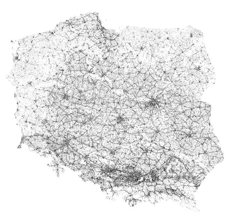
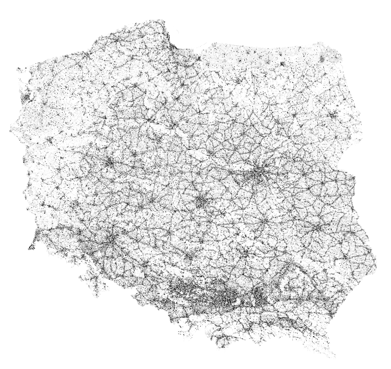
Figure 4: The LandScan population density in Poland (top), and virtual population density represented by density of households (bottom). Both data sets were created with 1 km resolution. Both sets show smaller population density in the NW and NE parts of the country, very high population density in the central-southern region of the country, and in some small concentrated areas corresponding to bigger agglomerations. The biggest conurbation areas are that of the capital city in the central-eastern part of the country and a highly populated and industrialized areas in the South. These are the most characteristic features of population density in Poland, and they are accurately well reproduced in our virtual society model.
- 4.3
-
The distribution of households' sizes, the distribution of children number in households (see Figure 5a), the distribution of age difference in couples (see Figure 5b), and the distribution of parents' age are all also well reproduced. Example 2,3,4, and 5-agent households are presented in Figure 5c. In the case of both, the distributions of the children number in households and the age difference in couples, data taken from NCB and from our model represent two different aggregation methods, therefore a direct comparison is not possible. More detailed descriptions of the aggregation methods are given in the figures' captions.
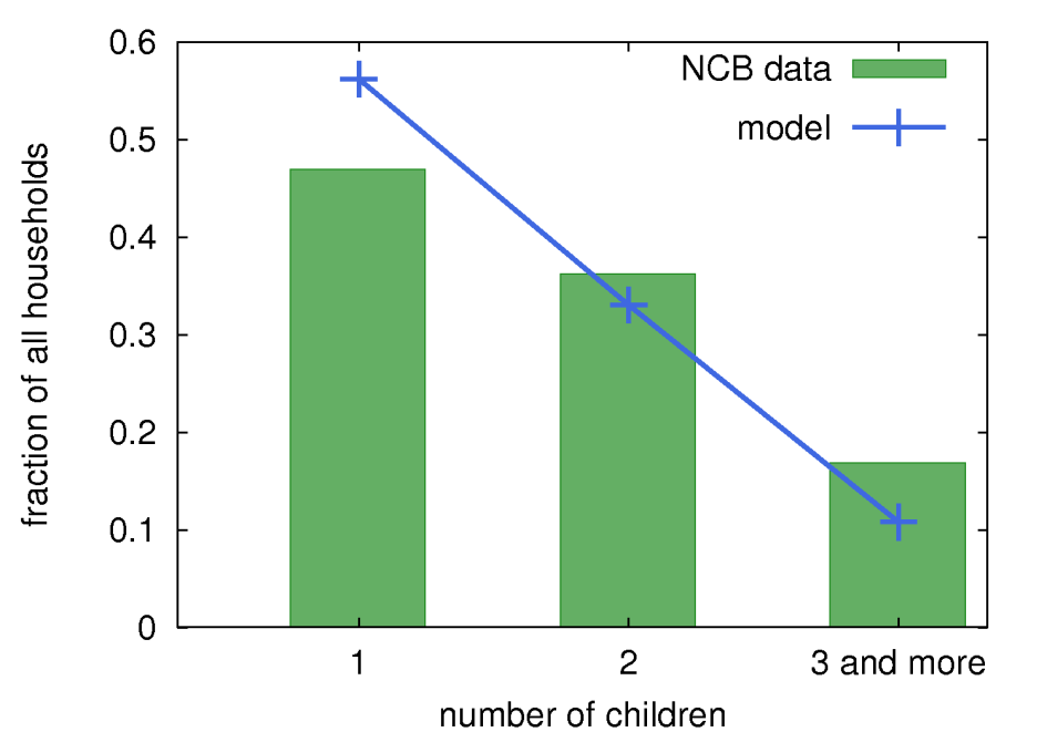
Figure 5a: The normalized distribution of the children number in households for the whole of Poland as given by census data (green histogram bins) and from the model described here (blue symbols, connected for clarity). One should note, that census data holds only the contracted information for the households with 3 and more children, so also for the sake of the comparison, the numerous households in the model were summed up to a single bin. 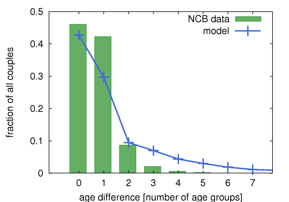
Figure 5b: The distribution of the age difference in marriages in Poland as given by census data (green histogram bins) and from the model described here (blue symbols, connected for clarity). One should note, that the data from the NCB contains the statistics collected among new marriages registered in the year 2002. The data are aggregated, and are given as the difference between age groups (spanning the time range of 5 years) of the two spouses, e.g. one can get the number of marriages between a member belonging to 19-24 years age group and a member belonging to the 25-29 age group. Hence, there must be an ambiguity in setting the particular age difference statistics expressed in years. Vertical axis gives the age group difference: 0 means that the couple belongs to the same age group, 1 and more means that they are from different age groups, e.g. 1 means that the spouses belong to two adjacent age groups (it means that one of the spouses is at least 1 day older and at most 9 years older than the other). On the other hand, the model described here yields a well defined histogram of the age difference between the most probable candidates for being a marriage-like couple within the entire society (not only new marriages). Hence, to correlate data from the model with the data taken from NCB, the former were aggregated into age group differences: 0-4 age difference within a (model) couple means the members belong to the same age group, 5-9 age difference - members belong to adjacent age groups, and so on. 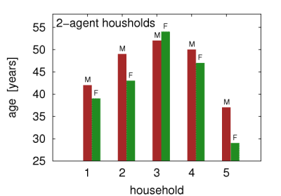
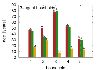
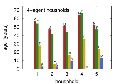
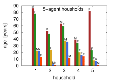
Figure 5c: Example virtual households created in this work. M and F symbols correspond to male and female agents, respectively. - 4.4
-
Distance to institution statistics
Within the virtual society created so far, the mean distances for pupils and students to travel to their respective schools, colleges, as well as for workforce to travel to their workplaces were calculated. In each case the distance was calculated just as a Cartesian distance between two points. The appropriate mean distance statistics were calculated at a commune, poviat, or voivodeship resolutions.
The mean household-workplace distance obtained from our model was 10.2 km. There is no detailed data on such distances provided by NCB, there is though a short analysis on the household-workplace distances for women in Poland (Jaros 2008), which yields the mean value of 9.2 km.Mean distances from households to schools
- 4.5
-
The results obtained for the three educational levels (primary and secondary schools, colleges) are presented in Figure 6 at a voivodeship resolution, within the context of population density in poviats.
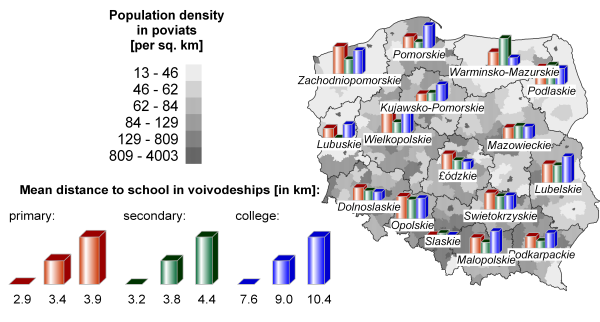
Figure 6: Results obtained within the virtual society: mean distance from household to school (primary, secondary, or college) in voivodeships (bars), and mean population density in poviats (hatch-map). Typically, the more densely populated a given voivodeship is, the more schools are available and hence, the shorter is the mean household-school distance. Thus, the pupils in Slaskie voivodeship in the South of Poland have the shortest distances to travel. This voivodeship is characterized by a rather uniform, high population density. The medium mean distances in Mazowieckie voivodeship (the one that includes the capital city of Warsaw) is the result of the relatively short distances in highly populated and abundant in schools capital city, and the relatively low population density and low school availability in the surrounding communes.
- 4.6
-
As a more detailed test case we chose Malopolskie voivodeship located in the southern Poland, mostly because of the surveillance statistics availability for this region (Guzik 2001; Guzik 2003). Figure 7 shows the availability of colleges in communes of Malopolskie voivodeship.
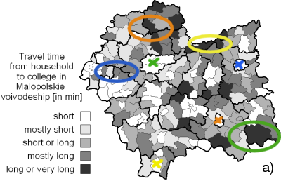
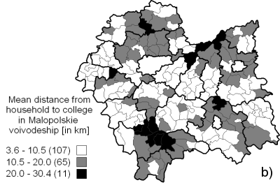
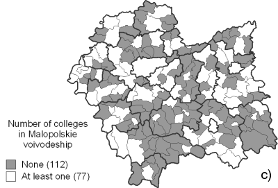
Figure 7: Colleges availability in Malopolskie voivodeship: a) the average time necessary to get to the college in villages or cities (data from the work of Guzik (2001)), b) the average household-college distance in communes obtained using the model described in this work, c) the presence of schools in the communes (data from the NCB). Figure 7a presents average time necessary to reach a college in communes of Malopolskie voivodeship in years 1998-1999. The original data (Guzik 2001) in the finer (village) resolution were projected on the commune territories. This survey relates to the timing of getting to schools and divide travel time into three categories: short - up to 45 minutes, long - between 45 minutes and 90 minutes, and very long - above 90 minutes. These times include also the time necessary to wait in the situation when the only public transportation means available arrive significantly earlier than the actual start of school classes.
Figure 7b contains the data obtained from the model described here, and presents the mean distance from household to college in each commune. Finally, Figure 7c shows the presence of schools in each commune (grey fields mark the communes without any colleges).
Figure 7b marks out several regions of rather poor school availability, expressed in long household-college distances. In the case of the South-East (green ellipse) and southern regions, the explanation may be the lack of schools in these regions shown in Figure 7c. This pattern is also visible in Figure 7a in the case of south-eastern region of Malopolskie voivodeship. The North (orange ellipse) and North-Eastern (yellow ellipse) regions of long household-college distances are also pointed out as the regions characterized by long time necessary to reach a school. There is also a small North-Western (blue ellipse) region visible in all three figures. Also, the short mean distances in the major cites of Malopolskie region are reproduced (see the marked major cities in Figure 7a with crosses).
One should note, that a complete correlation between time statistics (Guzik 2001) and distance statistics from this work is not possible, because the latter does not yet account neither for any exact road network, nor for any transport timetable, while the former (Guzik 2001) provides a detailed and extensive study of the exact travel times involved in educational availability in Malopolskie voivodeship. Nevertheless, some qualitative correlations are reproduced, despite the fact that only Cartesian travel distance have been implemented so far.Mean distance to RSU
- 4.7
-
As described in Methods section, the addition of the subsequent RSUs was constrained to the minimal distance of 2 km between the units. Consequently, the maximum number of the located units in any commune (see Figure 8) corresponds to the area of that commune. Therefore, Figure 8 reflects also the area size distribution of communes in the whole country.
Despite the high numbers of RSUs, the regions of northern and western Poland (described by a low population density and relatively big areas of the constituting communes) are represented by big mean distances to the rescue unit, as shown in Figure 9.
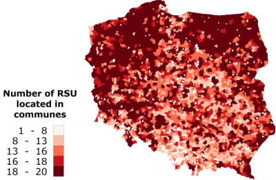
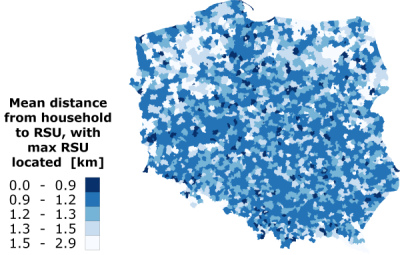
Figure 8: Maximal number of the RSUs located in particular commune. Figure 9: Mean distance between a household and a rescue unit in a commune, when maximum number of RSUs is located in the commune. Simplified economic analysis of the RSU system
- 4.8
-
Based on the models described so far, it is possible to carry out the preliminary economic analysis of the geo-referenced structure of RSUs distribution.
The most important factors that need to be balanced are the benefits related to the decrease of the mean household-RSU distance and the costs of creating any additional RSU in a commune. However, due to the inhomogeneous structure of population density, it is not a straight forward task to correctly estimate general benefits of establishing another RSU in a commune.
The mean distance from a household to the closest unit as a function of the number of RSUs in a commune is described here by a decaying function (named herein D). Function D is a reciprocal function, since the mean distance to RSU is inversely proportional to the number of located RSUs. It also depends on a commune topology. The following factors, among others, strongly affect the D-function: commune type (whether it is a rural, a urban, or a urban-rural commune), area of this commune and population density. Selected cases of D-function, presented as fits to the data, are shown in Figure 10.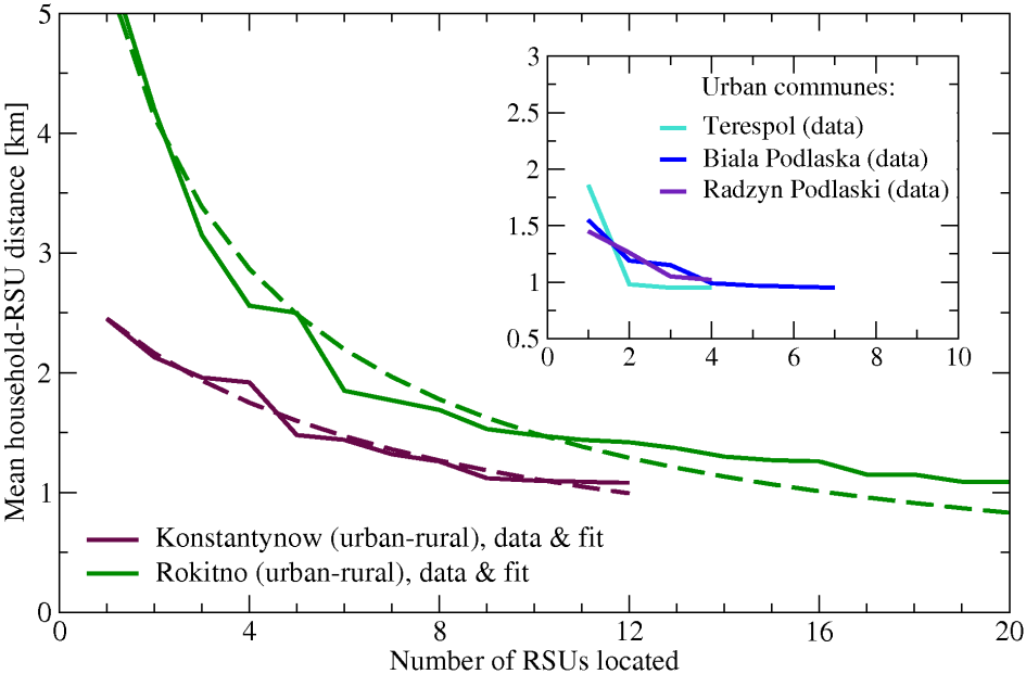
Figure 10: Examples of the dependence of the mean distance from household to rescue unit on the number of rescue units located in a commune for selected urban-rural communes (main plot) and urban communes (inset), together with the fitted curves in the case of urban-rural communes. No fits were done for the case of urban communes. Discrete data values (points) were connected for the sake of clarity.
- 4.9
- A good measure of the non-linearity of the D function in this case could be a root mean square difference (denoted as an rms difference) calculated between the linear function fitted to the initial and final point of the decay, and the decay data. Initial point's coordinates are defined by the mean household-RSU distance with one RSU located, final point's - by the mean household-RSU distance at the maximum number of RSU located. When rms difference values are small, the addition of a rescue unit in the commune considered results in the significant improvement of the accessibility to the RSUs. When rms difference values are high, only a few initial rescue units are beneficial because adding another RSU does not change much the mean distance to RSU.
Concluding remarks
- 5.1
- We reported here a robust, modular platform to create a large scale virtual society. The algorithms developed to create a network of virtual agents and objects of an appropriate type and properties, together with the imposed relationships among them, proved to be efficient.
- 5.2
-
First, the proper, countrywide, geo-referenced households size distribution was reproduced. Thus, the general descriptors of Polish society such as the total number of inhabitants or the percentage of both genders, together with the respective age distributions, were preserved. Further, the usage of the rules developed here yielded proper age and gender substructures in every household.
- 5.3
-
Within the proposed virtual society model, basic educational infrastructure was established, based on the commune-resolution statistical data regarding educational units - primary and secondary schools, colleges, and universities (not mentioned in the text). This constituted a preliminary contact map containing the information about pupils or students pertaining to a given educational unit. Similar work was performed regarding workplaces.
- 5.4
-
The resulting virtual structure permitted to perform an analysis of this structure. We presented several examples that included: mean distance to three types of educational unit statistics, as well as variability of the mean distance to rescue service units as a function of the number of the latter.
- 5.5
- The model implements a simple transportation model based on the approximate city network. Moreover, the software platform reported here is ready for the further implementation of road and railroad networks and corresponding traffic. Both features as well as the on-going epidemiological simulations are currently under development, and will be reported shortly.
Acknowledgements
- Authors were partially supported by the EU project SSPE-CT-2006-44405, also FR and MG were partially supported from the 352/6.PR-UE/2007/7 grant.
References
-
BAI X, Marinescu D C, Blni L, Siegel H J, Daley R A, and Wang I-J (2008)
A macroeconomic model for resource allocation in large-scale distributed systems, J. Parallel Distrib. Comput., 68 , pp.182-199 [doi:10.1016/j.jpdc.2007.07.001]
BALLAS D, Clarke G P, Dorling D, Rossiter D (2006) Using SimBritain to Model the Geographical Impact of National Government Policies, Geographical Analysis, 30, pp. 44-77
BECKMANN R J, Baggerly K, McKay M (1996) Creating synthetic baseline populations, Transportation Research A, 30, pp.415-429 [doi:10.1016/0965-8564(96)00004-3]
BERTOTTI M L and Delitala M (2006) On the qualitative analysis of the solutions of a mathematical model of social dynamics, Applied Mathematics Letters, 19, pp.1107-1112 [doi:10.1016/j.aml.2005.12.001]
BIRKIN M, Turner A, Wu B (2006) A Synthetic Demographic Model of the UK Population: Methods, Progress and Problems, Proceedings of the Second International Conference on e-Social Science, National Centre for e-Social Science, Manchester
CETIN N, Nagel K, Raney B, and Voellmy A (2002) Large-scale multi-agent transportation simulations, Computer Physics Communications, 147, pp. 559-564 [doi:10.1016/S0010-4655(02)00353-3]
DJIKSTRA E W, A Note on Two Problems in Connexion with Graphs, Numerische Mathematik, 1 (1959) pp. 269-271 [doi:10.1007/BF01386390]
DUNHAM J B (2005) An Agent-Based Spatially Explicit Epidemiological Model in MASON Journal of Artificial Societies and Social Simulation, 9(1)3 https://www.jasss.org/9/1/3.html
EUBANK S, Guclu H, Anil Kumar V, Marathe M, Srinivasan A, Toroczkai Z, Wang N (2004) Modelling disease outbreaks in realistic urban social networks., Nature, 429, pp.180-184 [doi:10.1038/nature02541]
CAUCHEMEZ S, Valleron A J, Boelle P Y, Flahault A, and Ferguson N M (2008) Estimating the impact of school closure on influenza transmission from Sentinel data, Nature, 452, pp.750-754 [doi:10.1038/nature06732]
FERGUSON N M, Cummings D, Cauchemez S, Fraser C, Riley S, Meeyai A, Iamsirithaworn S, and Burke D (2005) Strategies for containing an emerging influenza pandemic in Southeast Asia, Nature, 437, pp. 209-214 [doi:10.1038/nature04017]
FERGUSON N M, Donnelly C, and Anderson R A (2001) Transmission intensity and impact of control policies on the foot and mouth epidemic in Great Britain, Nature, 413, pp. 542-548 [doi:10.1038/35097116]
FERGUSON N M, Cummings D A T, Fraser C, Cajka J C, Cooley P C, and Burke D S (2006) Strategies for mitigating an influenza pandemic, Nature, 442, pp. 448-452 [doi:10.1038/nature04795]
FERGUSON N M, Galvani A P, and Bush R M (2003) Ecological and immunological determinants of influenza evolution, Nature, 422, pp. 428-433 [doi:10.1038/nature01509]
GALAM S (2004) Sociophysics: a personal testimony, Physica A, 336, pp.49-55 [doi:10.1016/j.physa.2004.01.009]
GERMANN T C, Kadau K, Longini I, and Macken C (2006) Mitigation strategies for pandemic influenza in the United States, Proc. Nat. Acad. Sci., 103, pp.5935-5940 [doi:10.1073/pnas.0601266103]
GOLDSTONE R L and Janssen M A (2005) Computational models of collective behavior, TRENDS in Cognitive Sciences, 9, pp. 424-430 [doi:10.1016/j.tics.2005.07.009]
GRANGER C W, Comparing the methodologies used by statisticians and economists for research and modeling, Journal of Socio-Economics, 30, pp.7-14 [doi:10.1016/S1053-5357(01)00089-0]
GUZIK R (2001) Wybrane problemy badawcze geografii spolecznej w Polsce, Kat. Geogr. Ekonom. Uniw. Gdanskiego, Gdynia, 2001, chapt. Dostepnosc szkolnictwa sredniego a szanse zyciowe w obszarach wiejskich, pp. 215-224.
GUZIK R (2003) Access to education and the knowledge-based economy in Poland: The regional perspective, in The Annual Anglo-Polish Colloquium "The Knowledge-Based Economy in Central and East European Countries: Exploring the New Policy and Research Agenda", SSEES-UCL, London.
HAMAMMI R, Frein Y, and Hadj-Alouane A B (2008) Supply chain design in the delocalization context: Relevant features and new modeling tendencies, Int. J. Production Economics, 113, pp. 641-656 [doi:10.1016/j.ijpe.2007.10.016]
HOGEWEG P (2007) From population dynamics to ecoinformatics: Ecosystems as multilevel information processing systems, Ecological Informatics, 2, pp. 103-111 [doi:10.1016/j.ecoinf.2007.01.002]
JANIC M (2000) Air Transport System Analysis and Modelling: Capacity, Quality of Services and Economics, Gordon and Breach.
JAROS R (2008) Psychologiczne, spoleczne i rodzinne aspekty mobilnosci kobiet na rynku pracy, report within the project From unemployment to employment - Women mobility at labour market maintained in the framework of European Social Fund.
KUTAKH A P and Fursova T I (2003) A simulation modeling system for estimation of the efficiency of new technologies and organization of railroad transportation, Cybernetics and Systems Analysis, 39, pp. 909-917 [doi:10.1023/B:CASA.0000020233.28801.b6]
LAKSHMANAN T R and Han X (1997) Factors underlying transportation CO2 emissions in the USA: A decomposition analysis, Transportation Research Part D, 2, pp.1-15 [doi:10.1016/S1361-9209(96)00011-9]
PABJAN B (2004) The use of models in sociology, Physica A, 336, pp.146-152 [doi:10.1016/j.physa.2004.01.019]
RANEY B, Voellmy A, Cetin N, Vrtic M, and Nagel K (2002) Towards a Microscopic Traffic Simulation of All of Switzerland, P.M.A. Sloot et al. (Eds), Springer Heidelberg. [doi:10.1007/3-540-46043-8_37]
RICHARDSON B C (2005) Sustainable transport: analysis frameworks, Journal of Transport Geography, 13, pp. 29-39 [doi:10.1016/j.jtrangeo.2004.11.005]
RICKERT M and Nagel K (2001) Dynamic traffic assignment on parallel computers in TRANSIMS, Future Generation Computer Systems, 17, pp. 637-648 [doi:10.1016/S0167-739X(00)00032-7]
STROUD P, Del Valle S, Sydoriak S, Riese J and Mniszewski S (2007) Spatial Dynamics of Pandemic Influenza in a Massive Artificial Society, Journal of Artificial Societies and Social Simulation 10(4)9https://www.jasss.org/10/4/9.html
SVENSON J E, O'Connor J E, and Lindsay M B (2006) Is air transport faster? A comparison of air versus ground transport times for interfacility transfers in a regional referral system, Air Medical Journal, 24, pp.170-172 [doi:10.1016/j.amj.2006.04.003]
ULENGIN F, Sule Onsel, Y. Ilker Topcu, Emel Aktas, and Ozgur Kabak (2007) An integrated transportation decision support system for transportation policy decisions: The case of Turkey, Transportation Research Part A, 41, pp.80-97 [doi:10.1016/j.tra.2006.05.010]