Sujai Kumar and Sugata Mitra (2006)

Self-Organizing Traffic at a Malfunctioning Intersection

Journal of Artificial Societies and Social Simulation vol. 9, no. 4
<https://www.jasss.org/9/4/3.html>

For information about citing this article, click here

Received: 07-Mar-2006    Accepted: 07-Jul-2006    Published: 31-Oct-2006

Abstract

Traffic signals and traffic flow models have been studied extensively in the past and have provided valuable insights on the design of signalling systems, congestion control, and punitive policies. This paper takes a slightly different tack and describes what happens at an intersection where the traffic signals are malfunctioning and stuck in some configuration. By modelling individual vehicles as agents, we were able to replicate the surprisingly organized traffic flow that we observed at a real malfunctioning intersection in urban India. Counter-intuitively, the very lawlessness that normally causes jams was causing traffic to flow smoothly at this intersection. We situate this research in the context of other research on emergent complex phenomena in traffic, and suggest further lines of research that could benefit from the analysis and modelling of rule-breaking behaviour.

Keywords:

Self-Organizing Systems, Complex Systems, Traffic, Emergent Behaviour, Agent-Based Modelling, Rule-Breaking

Introduction

1.1

Traffic jams are a problem in almost every major urban area in the world today. Some of the earliest research on the physics of traffic jams and traffic flows started over half a century ago (Lighthill and Whitham 1955) and has continued through the years using more and more sophisticated tools and techniques such as kinetic gas theory, fluid dynamics, and cellular automata, among others (for a comprehensive review, see Helbing 2001). Most of this research deals with aspects of traffic that are mechanical (traffic densities, traffic signals, grid layouts, etc). In addition, a fair assumption that most 'traffickers' make is that the system works as designed, and that it is the design that needs to be studied and improved.

1.2

However, in many developing countries, including India (where the authors reside), traffic signals often fail — mostly due to a power failure, but occasionally, even when there is power, they freeze in a particular configuration because of poor-quality switching equipment.

1.3

One of the authors was caught in just such a situation one evening where the traffic lights for two directions at a three-way intersection were stuck showing red while the third direction was always green, and observed that traffic actually seemed to be flowing quite smoothly in all directions. There would be a wait, but then a platoon of cars would move forward and through the intersection and the ones behind would wait, just as if the traffic lights were working perfectly. Initially, the author assumed that a policeman was aware of the malfunctioning lights, and was guiding traffic at the intersection, but when he approached the intersection, he was surprised to find no policeman there and each stream of traffic moving in bursts, by turn.

1.4

Before we go into more details, it is important to note that this is not analogous to situations where there is no traffic light, or where a traffic light is not working, and people are following the "stop" rule. Internationally, the "stop" rule is that a car should stop at an intersection, allow cars that stopped earlier at the intersection to move first, and then move itself. The "stop" rule is an example of well defined cooperative agent behaviour, but there is no emergent or complex behaviour in that case because the global behaviour is a scaled up version of the local behaviour.

1.5

On the other hand, our scenario was an example of traffic flows that take turns and move in platoons without any regulatory or timing inputs like traffic signals or traffic policemen. It was this collectively complex behaviour that we set out to model. This quote from Helbing and Huberman (1998) best sums up the phenomena that we are trying to replicate:

In many social situations, decisions made by individuals lead to external effects that may be very regular, even without a global coordinator. In traffic, these decisions concern when to accelerate or brake, to overtake or to enter a busy multi-lane road, while trying to get ahead as fast as possible, but safely, under the constraints imposed by physical limitations and traffic rules. At times these behaviours give rise to very regular traffic patterns, as exemplified by the universal characteristics of moving traffic-jam fronts or synchronized congested traffic. These phenomena are in contrast with usual social dilemmas, where cooperation in order to achieve a desirable collective behaviour hinges on having small groups or long time horizons.

1.6

In our case, one of the key points of departure from this description is that the individual agents don't follow traffic rules. In India, even careful drivers have a tendency to be impatient with a red light (perhaps because they have previously experienced traffic lights that were 'frozen' in the same configuration), and they eventually break the rule by crossing a red light that has stayed red for too long. In the model that we present, we show how this lawlessness can still lead to relatively organized behaviour.

1.7

This paper is organized as follows. The next section (section 2) provides a brief history of traffic simulations and how the current simulation relates to them. Section 3 describes the components of the model, its environment, and the behaviours of the agents in the model. Section 4 presents the experiments done with the model and the main results that were obtained, while Section 5 presents a comparative analysis of three very different signal-types at the intersection. Lastly, in section 6, we discuss how the given model is an example of a complex system, what variations we would like to try on the model in the future, and how we could use the results from this study in related research areas.

Relation to existing traffic simulations

2.1

Traffic models and simulations have helped provide insights into many phenomena like 'phantom traffic jams' which propagate backwards even when there is no obstacle in the way (Nagatani 2002), speed limits that can speed up traffic (Treiber and Helbing 2001), pedestrians moving in opposite directions organizing themselves into lanes (Hoogendoorn and Daamen 2004), and so on.

2.2

Over the years, researchers have focussed on different aspects of traffic — the flow of vehicles on single-lane and multi-lane freeways, the formation of jams, the occurrence of deadlocks in city traffic, and the optimization of traffic flows using traffic lights or other measures. Only a small fraction of these papers concentrate on describing the effect of traffic lights on congestion (Brockfeld et al 2001; Gershenson 2005; Spall and Chin 1997).

2.3

In this paper, we describe a single real-world phenomenon — self-organizing traffic at a malfunctioning intersection where the lights are frozen in a particular configuration. To the best of our knowledge, this kind of model or description has not been attempted before. The closest existing research we can think of is Gershenson's (2005) work on self-organizing traffic lights where smooth traffic flows are maintained despite the absence of any centralized control system with complete information, but his traffic lights work as designed, and his vehicles follow traffic rules, whereas our model investigates the interaction of malfunctioning signals and rule-breaking behaviour.

2.4

As Helbing (2001) has pointed out, several modelling techniques and tools have been used to study traffic ranging from differential equations to gas kinetic theories to liquid dynamics, and, with the advent of powerful computers, cellular automata (CA). We chose to work with a CA model of traffic that is closely related to the first CA traffic model by Nagel and Schreckenberg (1992) in that each vehicle occupies a cell on a grid of squares, and the grid is updated on each time-step following certain simple rules in order to determine the positions of the vehicles. This is described in more detail in the next section.

Model description

3.1

Our model is of a three way t-shaped intersection where we only simulate those traffic flow directions that intersect other traffic flow directions and could cause gridlocks.

3.2

The traffic signal could be working normally or malfunctioning, as described in more detail later in this section. Drivers have to wait when the traffic signal is red for their lane, but when the waiting time exceeds a certain wait-time-limit, we assume that a driver gets impatient and starts to cross the intersection even though the light is red. This lawlessness is the key aspect of this model and reproduces some interesting real world phenomena.

3.3

The model was implemented using NetLogo 3.0, a cross-platform multi-agent programmable modelling environment (Wilensky 1999). NetLogo is written in Java and is designed to give exactly the same results no matter what hardware it is run on. The model can be viewed using any Java enabled browser and its parameter space can be explored at http://www.ylog.org/complex/traffic/sot-2006-07-01-1930.html (Kumar 2006)

3.4

All models are simplifications of reality, and our model is no exception. In the next few sub-sections, we present the simplifications we assumed, and the reasons for making these assumptions.

Environment

3.5

The environment consists of a square grid made up of 31 × 31 patches or cells. NetLogo uses the term 'patch' so that is the term we use in the subsequent sections as well. The precise size of the grid is immaterial, as traffic self-organizes in this model across different-sized grids.

3.6

Following the assumptions made in the Nagel and Shreckenberg (1992) model (abbreviated as NaSch), each patch can be assumed to be about 5m in length (i.e., slightly larger than a car).

3.7

All vehicles are assumed to be the same size in this highly simplified model. In the discussion section we propose that a more realistic model of the kind of chaotic traffic one regularly sees on a Delhi road would have to include a wide variety of vehicle sizes from bicycles to container trucks.

3.8

A patch can be empty or occupied by exactly one car. Collisions are explicitly forbidden in this model. When cars move, they move exactly one patch per time-step.

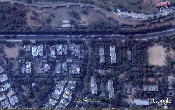
Figure 1. a) Overview of intersection, showing traffic flows, unsimulated lanes, and how vehicles wait at, and cross the intersection. b) The same intersection, as seen on Google Earth (download placemark at http://www.ylog.org/complex/traffic/kumar-mitra-selforg-traffic-malfunctioning-intersection.kml)

3.9

A time-step in the model can be assumed to be a little less than 1 second in real life. A speed of about 5m/s (about 18km/hr) might seem a bit slow for a car but this is a model of a crowded intersection, so that speed is certainly plausible.

3.10

This model does not account for speed variations the way the NaSch model does. Speed variations definitely contribute to jams and their resolutions (Koshi et al 1983; Herrmann and Kerner 1998; Helbing and Schreckenberg 1999), but we are interested in driver lawlessness in their non-stopping behaviour, not in their over-speeding or slowing tendencies. The sub-section on agent-behaviour presents this in more detail.

3.11

In this paper, we present a three-way high traffic density intersection because the phenomenon was originally observed at such an intersection. Although we present one experiment in the next section with a very low traffic density, we are primarily interested in how dense traffic resolves itself at a malfunctioning intersection.

3.12

All vehicles drive on the left, but the model and the environment is symmetric and traffic can be assumed to be on the right without any loss of generality.

3.13

All three roads (from the North, East, and West) have four lanes each, two each in opposing directions. Each lane is labelled with two directions — the direction from where traffic is coming, and the direction to which traffic is moving.

3.14

Only one lane from each direction is simulated in this model, because the other lane is assumed to have a smooth flow (since there is no interference from any of the other lanes). Thus the lanes simulated are East-North, North-West, and West-East, and the lanes ignored are East-West, North-East, and West-North.

Variables

3.15

Several parameters in the model are variables that can be tweaked or set to extremes in order to explore the parameter space of the model.

car-density

A global parameter that ranges from 0 to 1. This variable specifies how often new cars are generated at the start of each lane, provided there is room for the cars to be created. For most values of the density variable, the effective density remains maximal because if the traffic is backed up to the edge of the simulation space, then there is no way for there to be an empty space. A suitably large simulation space will ensure that backed-up traffic does not extend to the edge of the simulation space, thus allowing the actual density to reflect the parameter value more closely.

wait-time-limit

The number of time-steps that a driver spends waiting before becoming impatient and deciding to break the rule by crossing a traffic light.

signal-type

Used by the experimenter to specify the different types of traffic signals that the model supports. Values include:

Normal

The signal works as it should — traffic from each direction is Green in turn while the others remain Red.

All Red

Malfunctioning signal. All directions remain Red all the time.

All Green

Malfunctioning signal. All directions remain Green all the time.

North Green, rest Red

Malfunctioning signal. The traffic lights remain stuck in this configuration.

North Red, rest Green

Malfunctioning signal. The traffic lights remain stuck in this configuration.

West Green, rest Red

Malfunctioning signal. The traffic lights remain stuck in this configuration.

signal-cycle-time

If the signal-type is Normal, then this variable determines the number of time steps after which the signals cycle through the same configuration again. For example, if this parameter is 60, then traffic from each of the three directions gets 20 time-steps to move. To be precise, the traffic-light for each direction stays Green for 18 time-steps (the remaining 2 time-steps are to allow any straggling cars to finish crossing the intersection)

Agent Behaviour

3.16

An agent in this simulation is an individual vehicle. Each agent is programmed to behave in exactly the same way, because we wanted to keep the underlying local rules as simple and standard as possible, but see if they could allow complex behaviour to emerge globally.

1. Moving forward

   Rule 1.

   If a vehicle is not at a traffic light, it tries to move forward to the patch in front in one time-step, provided the patch ahead is not blocked, otherwise it stops on the current patch.

   Rule 2.

   If a vehicle is stopped for any reason, its waiting time counter increases by 1 for each time-step spent stopped.

   Rule 3.

   If a vehicle is changing its direction of motion at the intersection (e.g, in the East-North or North-West traffic flows), it turns right by 45 degrees, but still moves exactly one patch in that direction per time-step. The distance travelled in this case is Sqrt(2) × Length of patch. In other words, the velocity is discrete — either 0 or 1 patch or Sqrt(2) patches per time-step.

   Figure 2. Close-up of intersection, showing distance travelled by a vehicle when moving straight or turning across the intersection

   Rule 4.

   If the patch ahead is blocked, then the current vehicle stops and waits until it is clear.

2. Checking signal

   Rule 5.

   In all cases, if a vehicle reaches a traffic light, and finds more than 5 vehicles in the intersection, it waits. The geometry of this model (Fig. 3) fixed this number at 5 because a higher limit is simply not possible in the intersection without instantly causing a gridlock where no vehicle can move at all.

   Figure 3. Close-up of intersection. The darker colours show patches in the intersection which are either at a traffic light, or are crossed by more than one traffic flow

   Rule 6.

   If a vehicle reaches a green light, it continues through the intersection towards the planned-for direction (e.g., a vehicle in the North-West traffic flow coming from the North will turn right towards the West as planned).

   Rule 7.

   If a vehicle reaches a red light, it stops and waits (and the waiting time counter increases as specified in Rule 2)

   Rule 8.

   If a vehicle is at a red light, and the waiting time exceeds the wait-time-limit, the driver get impatient and moves into the intersection (provided Rule 5 is not violated).

Simulation Experiments

4.1

In this section we present some runs in detail that we observed with different signal types and different wait-time-limit, signal-cycle-time, and car-density parameters. The first two experiments A and B describe situations where the traffic lights work normally, but where the drivers are more patient and less patient respectively. Experiment C deals with the situation where the lights malfunction and remain frozen in a configuration where one direction remains green all the time while the others stay red. This is the situation that the authors observed in real life and based on which this model was created. The final two experiments D and E in this section describe two very different scenarios as contrasts — with lights malfunctioning where all sides remain green, and with all drivers following the international stop rule where they wait for their turn to cross the intersection.

4.2

Only individual runs are present in this section, and a detailed analysis of an aggregate of 100 runs for each scenario is presented in Section 5.

Normal traffic lights with high wait-time-limit

4.3

We begin with the default ideal scenario — that all traffic lights work as planned. We use this first scenario to generate an average speed graph for each traffic flow (at each time-step), and for the intersection as a whole. This graph can then be compared with graphs generated in the other simulation experiments where we simulate malfunctioning lights, try different waiting-time parameters, etc.

4.4

Note that each of the following graphs represents one run of the simulation. We present individual runs to give the reader a feel for how the simulation behaves. In the analysis in Section 5, we present aggregate data across hundreds of runs to demonstrate that the turn-taking behaviour we observed was not an isolated phenomenon in just one run of the simulation.

Figure 4. signal-type: Normal; signal-cycle-time: 60 time-steps; car-density: 1.0, wait-time-limit 60 time-steps

4.5

The first 1000 time-steps are shown. Each plot point represents the average speed (measured in patches or cells per time-step) of all cars in a particular traffic flow, averaged over the plot-window or plot resolution — in this case, the previous 20 time-steps. The highest speed possible for each traffic flow is 1.0 patches/time-step, implying that every car moved one cell forward in that simulation time-step.

4.6

As expected, the different traffic-flows take turns peaking because the corresponding traffic lights turn green in the same order every 20 time-steps. Initially, the average speed of each traffic flow is high because none of the cars have had to stop in the first few time-steps as they approach the intersection.

4.7

The wait-time-limit was deliberately kept fairly high so no driver's waiting time would cross that limit, and they wouldn't get impatient and break rules. In Experiment B, we will explore a Normal signal-type with low wait-time-limit as well.

4.8

If we increase the plot-window from 20 time-steps to 60 time-steps, we see the curves becoming smooth, and the three individual traffic flows are almost identical. They are not perfectly identical because the model updates the locations of each agent at random within one time-step to prevent any artefacts that might be due simply to the update order.

Figure 5. signal-type: Normal; signal-cycle-time: 60 time-steps; car-density: 1.0. Same parameters as Fig. 4, except that the plot window is 60 time-steps instead of 20

4.9

Changing the signal-cycle-time only changes the frequencies of the peaks. Figure 6 shows how the frequency of the peaks is halved when the signal-cycle-time is doubled to 120 time-steps from 60 time-steps.

Figure 6. signal-type: Normal; signal-cycle-time: 120 time-steps; car-density: 1.0. Same parameters as in Fig. 4, with the signal-cycle-time doubled

4.10

Figure 7 shows the effect of reducing the traffic density. The combined average speed of all three traffic streams goes up, as cars have to wait for a shorter period of time in this case, but the curves remain essentially the same as in Figure 4. However, the overall throughput measured in number of cars passing through the intersection per time-step does go down as there are fewer cars.

Figure 7. signal-type: Normal; signal-cycle-time: 60 time-steps; car-density: 0.1. Same parameters as in Fig. 4, with the car-density reduced

Normal traffic lights with low wait-time-limit and high signal-cycle-time

4.11

If the traffic lights work normally, but the drivers have a shorter wait-time-limit than the signal cycle time (either because these drivers get impatient really fast, or the signal takes longer than one would normally expect to change), then the system again gridlocks rapidly, as seen in Figure 8.

Figure 8. Gridlock configuration with no further movement possible

4.12

This scenario is occasionally visible on the roads of Delhi, but is rarer than the case where all traffic lights freeze in a particular configuration.

Figure 9. signal-type: Normal; wait-time-limit: 40 time-steps; signal-cycle-time: 180; car-density: 1.0

4.13

Repeated runs with these parameters showed that the traffic gridlocked (Fig. 9) on every single run, usually within 500 time-steps. However, if the wait-time-limit is equal to, or only a little less than the amount of time that the light stays green for each direction (one-third the signal-cycle-time), then the system works as expected, despite the lawlessness. In Figure 10, the wait-time-limit is 55 time-steps, which is only 5 time-steps lower than the 60 time-steps for which the light stays green in each direction.

Figure 10. signal-type: Normal; wait-time-limit: 55 time-steps; signal-cycle-time: 180; car-density: 1.0; plot-window: 60 time-steps

Malfunctioning traffic lights with one direction remaining Green

4.14

This scenario most closely mimics the real-life situation that inspired this model. When the traffic lights malfunction, and are frozen forever in a configuration where traffic from the North always get a Green light while the other two directions always get Red, then the traffic flow graph in Figure 11 is seen.

Figure 11. signal-type: North-Green, Rest Red; wait-time-limit: 120 time-steps; car-density: 1.0, plot-window: 40 time-steps; signal-cycle-time is immaterial as this is a malfunctioning signal

4.15

In Figure 11, traffic flow from the North to the West has the highest throughput which is expected as that light remains Green the entire time. Traffic from the East and the West initially waits at the intersection because the light is Red for them (Point A, Fig. 11), but when the wait-time-limit of 120 time-steps (double the normal signal-cycle-time) is exceeded, drivers get impatient and start to cross the intersection as and when they get a chance. All the cars from the East and West have been waiting together, so they all reach their wait-time-limits at about the same time, and start moving together across the intersection (Point B, Fig. 11). Once the initial group of waiting cars has crossed the intersection, new vehicles which arrive at the intersection from the East and West wait at the Red light because their wait-time-limit has not yet been reached, causing the average speed for traffic from the East and West to drop (Point C, Fig. 11). This behaviour has a direct parallel in the real world where cars that arrive at the intersection don't know that it is not working (because the traffic in front of them did move eventually), and are thus content to wait for a while until their patience levels are tested. After these vehicles reach their wait-time-limit, they start across the intersection together again.

4.16

Initially, for approximately the first 1000 time-steps, vehicles from the East and West wait at, and move across the intersection at almost the same time (from Point A to Point D in Fig. 11). However, from about 1000 to 2000 time-steps, we see that those two traffic flows have started to take turns in crossing the intersection (the two curves peak at different times). The effect becomes even more pronounced from 2000 to 4000 time-steps in Figure 12.

Figure 12. signal-type: North-Green, Rest Red; wait-time-limit: 120 time-steps; car-density: 1.0, plot-window: 40 time-steps; 2000 to 4000 time-steps

4.17

What causes the East and West traffic flows to take turns even though their average speeds were initially synchronized? We examined several runs of the simulation closely, and concluded that the random order in which the cars move into the intersection breaks the symmetry of the system. Although both traffic flows (from the East and the West) initially waited together at the intersection, cars from one direction would enter the intersection before cars from the other direction (because the positions of the cars within one time-step are updated at random). If, on a particular run, after a period where both Eastern and Western traffic flows waited at the intersection, a car from the East entered the intersection first, then a car from the West might be forced to wait (because of the rule preventing too many cars from entering the intersection). Even this short extra wait can break the symmetry of this system because all cars behind the first car from the West would then be forced to wait an extra time-step. These small differences in waiting time add up until one traffic flow has an average wait-time that is higher than the other. Over time, that set of cars will reach the wait-time-limit faster and start moving across the intersection sooner the next time that both traffic flows are waiting at the intersection.

4.18

This turn-taking behaviour is a good example of a complex system in real world social behaviour because it does not rely on a central regulatory authority to coordinate the turns. It emerges out of individually selfish and rule-breaking behaviour where each individual vehicle only has information about the vehicle in front.

4.19

When we let the simulation run longer, another interesting phenomenon that emerged was the oscillation between platoons from the East and West moving together, and taking turns. Figure 13 shows the simulation from 4000-6000 time-steps. After 4000 time-steps, the East and West traffic flow throughput curves again start peaking at the same time. Even when we let the simulation run for a further 10,000 time-steps, we observed these two platoons oscillating between the two states — moving together and taking turns.

Figure 13. signal-type: North-Green, Rest Red; wait-time-limit: 120 time-steps; car-density: 1.0, plot-window: 40 time-steps; 4000 to 6000 time-steps

4.20

The graphs till now have provided details of a single run of the model. Repeated runs did not always result in turn-taking behaviour. On several runs, the traffic gridlocked (as in Fig. 8) after a few time-steps. Figure 14 shows the proportion of 100 runs with the same parameters (signal-type: North-Green, Rest Red; wait-time-limit: 120 time-steps; car-density: 1.0) but different wait-time-limits (ranging from 30 to 120 in increments of 10 time-steps) that ended in gridlock.

Figure 14. Proportion of runs that ended in gridlock for differing wait-time-limits, for signal-type: "North-Green, Rest Red", and traffic density 1.0

4.21

At low wait-time-limits (i.e., when drivers are very impatient), the simulation gridlocks almost every time. The probability of gridlock occurring goes down as the wait-time-limit increases, but beyond a wait-time-limit of 90 time-steps, it starts increasing again. The gridlock proportion graph is compared with other signal-types in Section 5.

4.22

The simulation graphs till now showed average speed graphs for single runs of the model with different parameters. Figure 15 is an aggregate representation of 100 runs of the same model. It is a distribution of the absolute differences in speed for each time-step in each run of the model (analyzed collectively). Turn-taking behaviour is evident as a high proportion (0.457) of the total number of time-steps show a speed difference greater than 0.2. We compare this distribution with distributions for other signal types in more detail in the analysis in Section 5.

Figure 15. Distribution of absolute differences in average speed for East and West traffic flows, for each time-step, across 100 runs, with wait-time-limit 120 time-steps

4.23

If we reduce the wait-time-limit for the simulation, we see a reduction in the gap between the average speed curves in Figures 11, 12, and 13. Traffic from the directions with red lights will wait less, and thus their average speeds will increase.

4.24

Keeping the rest of the parameters the same as in Figure 11, Figure 16 shows the wait-time-limit reduced to 90 time-steps, while Figure 17 shows a wait-time-limit of 30 time-steps.

Figure 16. signal-type: North-Green, Rest Red; wait-time-limit: 90 time-steps; car-density: 1.0

Figure 17. signal-type: North-Green, Rest Red; wait-time-limit: 30 time-steps; car-density: 1.0

4.25

When the wait-time-limit is reduced to 90 time-steps (Fig. 16), the turn-taking self-organizing behaviour is still seen after about 1000 time-steps, but once the wait-time-limit is reduced to 30 time-steps, the platoons become smaller and are no longer visible on the plot, taking turns to cross the intersection (Fig. 17).

4.26

Reducing the wait-time-limit to 0 is essentially the same scenario as that of a malfunctioning signal with all lights staying Green all the time. This is described in the next sub-section. The average speed curves for the three directions become identical to the graph in Figure 18 and there is no turn-taking behaviour visible.

4.27

The chances of gridlock also increase as we reduce the wait-time-limit and the simulations approach the "All Green" scenario in Figure 18 in the next sub-section.

Malfunctioning traffic lights with all directions remaining green all the time

4.28

Figure 18 shows the average speeds of each traffic-flow in one run of our model when all the traffic lights are Green and frozen in that configuration.

Figure 18. signal-type: All-Green; wait-time-limit: 120 time-steps; car-density: 1.0, plot-window: 20 time-steps

4.29

The plots stop after about 100 time-steps in Figure 18 because a gridlock occurs (as in Fig. 11) where no traffic can move further because of the rules of our model, and the simulation halts.

4.30

This scenario is not an example of a self-organizing system because there is no emergent global behaviour that is qualitatively different from the local behaviour of individual vehicles. The average speeds for each direction all remain at about the same level until the simulation halts, with no evidence of turn-taking behaviour. Every vehicle tries to get through the intersection when it can, only pausing if there is another vehicle in front that prohibits further movement.

4.31

The scenario with all lights green all the time directly parallels the real world behaviour of traffic at an intersection where no lights are working and everyone tries to get ahead. Unlike some countries where drivers automatically follow the 'Stop' rule when they encounter malfunctioning traffic lights, a situation like this in India invariably ends in a gridlock as in the simulation, and is only cleared when a traffic policeman or concerned citizen steps into the fray and starts directing traffic.

4.32

Unlike the case where the traffic lights worked normally and the number of times that gridlock occurred was dependent on the wait-time-limit, in this case the traffic gridlocked every single time (detailed comparison in Section 5).

International Stop Rule

4.33

The graphs in the previous section mean little unless we have something to compare them with. Drivers who follow the international stop rule at an intersection are, in a sense, behaving most unlike the impatient drivers in the previous scenario, because they follow rules and don't barge through an intersection when they get impatient. The stop rule requires drivers to allow a car from another direction that reached the intersection first, to cross the intersection first. Traffic never gridlocks at this intersection, but it also passes through the intersection at a much lower overall average speed (Fig. 19). The simulation in Figure 14 also shows almost identical average speeds for each traffic flows. Although the cars do take turns at the intersection, the overall traffic flows don't take turns, moving in platoons, as they did in the case where the traffic lights functioned normally, or as in the previous section, where the drivers were impatient and the traffic lights were malfunctioning.

Figure 19. signal-type: Stop rule; wait-time-limit: 120 time-steps; car-density: 1.0, plot-window: 20 time-steps

Analysis

5.1

In the previous section, we presented individual runs of the model in detail with different signal-types and different parameters. In this section, we present a comparison of three signal-types.

5.2

Table 1 compares the following three signal-types: normal traffic lights, malfunctioning traffic lights with one direction remaining green, and traffic following the stop rule.

5.3

Each signal-type was run with 10 different values of the wait-time-limit parameter, ranging from 30 time-steps to 120 time-steps in increments of 10 time-steps. For each of these parameter settings, we allowed the model to run 100 times resulting in a total of 1000 runs of the model for each signal-type.

Table 1. Comparisons between three signal-types

5.4

As the comparisons indicate, the Stop Rule is the most effective at preventing gridlocks. A gridlock can never happen by the very definition of the rule. However, the total average speed of all the cars passing through the system is very low compared to the other two cases. Even in the case of normally functioning traffic lights (Table 1, Cell A1) — if people are impatient and lawless, that is, they have a low wait-time-limit, then there is a high incidence of gridlock.

5.5

Rows B and C in Table 1 are indirect indicators of turn taking behaviour., for each time-step the absolute difference in average speed between the East and West traffic flows is taken. There will be lower differences if there is no turn-taking behaviour and higher differences if platoons of cars go through the intersection. Large platoons (e.g., more than 20-30 cars at a time) going through the intersection show a speed difference of about 1 cell per time-step. Smaller platoons (5-10 cars at a time) show a speed difference of 0.3 — 0.5 cells per time-step. In the Stop Rule, a platoon is of size 1, and the speed difference is typically only about 0.25 cells/time-step. Row B shows a distribution of these speed differences and Row C shows the proportion of total time-steps considered which had a difference greater than 0.2.

5.6

Rows D and E in Table 1 show how throughput of the system changes with different wait-time limits. The more impatient drivers are (lower wait-time limits), the faster the overall traffic flows are, but the traffic also ends up in gridlock more often.

Discussion

6.1

The highly simplified model we have presented in this paper is fairly successful in mimicking the real-world self-organizing behaviour of traffic that we observed at a malfunctioning intersection. A one-line summary of this paper's simulation experiments could be "Lawless behaviour at an intersection with malfunctioning traffic-lights can lead to self-organized smooth traffic flows". The word 'can' is important in the previous statement as such behaviour could also lead to gridlock. We hope readers will try out the NetLogo simulation (Kumar 2006) that allowed us to replicate a counterintuitive phenomenon and show that it was a robust model valid for a wide range of parameters and not simply an artefact of a particular traffic density, signal period, or wait-time limit. More importantly, it highlighted the need to study situations where things do not happen as designed, to see how robust a system is, or can be.

6.2

No model can mimic reality perfectly, but, by changing only the wait-time parameter, we were also able to observe other classes of behaviour that are seen at real intersections where the individual drivers have a tendency to be lawless, thus lending further credibility to the model's validity.

6.3

In this discussion, we focus on three aspects of this model — how it is an example of a complex system, what other variations could be attempted, and other types of research that could benefit from this kind of modelling.

Complex emergent behaviour

6.4

Self-organizing traffic is seen in the situation where the traffic lights malfunction and remain frozen in a configuration where one direction is always green, while the others always stay red (Figs. 11, 12, and 13).

6.5

The turn-taking behaviour of the traffic without any centralized regulatory authority is an example of complex emergent behaviour. In this sub-section, we compare the characteristics of complex and self-organizing systems as proposed by several researchers (Camazine et al 2001; Gershenson and Heylighen 2003; Fewell 2003), with the characteristics of our system:

1. There are many elements in the system acting in parallel
2. The elements only have local interaction or local information, they are not individually in control of (or in some cases, even aware of) activity at a higher level
3. Able to withstand perturbations
4. Multiple stable attractor states in the state space (also an example of symmetry breaking). The platoons from the East and the West oscillate between taking turns and crossing the intersection together.
5. Away from/far from equilibrium (i.e. the system is not in its lowest energy state). The lowest energy state occurs when the traffic gridlocks and no vehicle can move any more.
6. Open to environment (free flow of energy/ information, dissipative structures). Free flow of incoming traffic. And the system organizes it into platoons and sends them on their way.
7. No single unit or non-communicative subset of units can achieve the system's goal as well as the collection can at high traffic densities.
8. The elements of the system use positive and negative feedback to regulate themselves. Positive feedback in this case is the wait-time-limit, which, coupled with the lawless behaviour, urges the drivers to move forward, while the traffic light acts as a negative feedback, preventing vehicles from moving forward.

Variations of this model

6.6

By the very definition of the term, a model is an attempt to mimic a simplified version of reality. In our example of self-organizing traffic at malfunctioning traffic lights, several simplifications were made to try and design a simulation that would be as simple as possible but still demonstrate the observed behaviour. In this sub-section, we present several possible variations of this model that could be of potential interest.

1. Physical variations

   One possible limitation of the model is that each vehicle is physically too simple — it does not even account for varying vehicle velocities. In addition, all vehicles have exactly the same size. Varying these physical aspects of the vehicles could have an interesting effect on how often jams and gridlocks occur and how fast they dissolve. For example, different sized vehicles might cause gridlocks because smaller vehicles might fill the gaps between larger vehicles and prevent any further movement. On the other hand, smaller vehicles might be able to better utilize small gaps in order to escape a jam, and thus contribute to clearing the gridlock.

2. Behavioural variations

   An infinite range of behavioural variations is possible. We have only considered one kind of behaviour where lawless drivers jump traffic lights when their vehicles stay stopped for a time-period longer than their wait-time-limit.

   One behaviour that is often observed around the world but not accounted for in this model is the tendency for vehicles to change lanes when confronted with congestion in their own lane, or to change direction altogether and choose a different route.

   Following the terminology of the classic Prisoner's Dilemma, drivers in India sometimes even switch to the lane going in the opposite direction because they want the immediate benefit of 'defecting', without appreciating the cumulative long-term effect of 'cooperating' with other vehicles.

   Such behaviours would be interesting to model but it is difficult to see how they would lead to self-organizing behaviour.

3. Environment variations

   Our simulation is only applicable to a three-way intersection where the traffic lights might freeze in a particular configuration. However, modelling other breakdown or malfunctioning situations — such as lane closures on a narrow mountain road, or the complete absence of traffic signals at a large intersection, could throw up some interesting insights as well into whether traffic might be able to flow efficiently in those cases as well in the absence of a regulatory system.

Related research

6.7

This model could be a good starting point for other scenarios that deal with the sustained, jam-free movement of independent agents, such as data flow management in packet networks, and crowd control in stadiums. In such scenarios, it could be useful to study, analyze, predict and plan for breakdowns of the intended design when agents do what they are not supposed to do either because of stress or because of other forces (in our case, they jump traffic lights).

6.8

It could also make an interesting case for studying more chaotic rather than more ordered social systems, because systems at the edge of chaos have a wider solution space to explore (Kauffman 1993). We are tempted to speculate that building in, or allowing for 'lawlessness' might lead to more robust, flexible and adaptive systems.

References

BROCKFELD, E., Barlovic, R., Schadschneider, A., & Schreckenberg, M. (2001). Optimizing traffic lights in a cellular automaton model for city traffic. Physical Review E, 64:056132.

CAMAZINE, S., Deneubourg, J. L., Franks, N., Sneyd, J., Theraulaz, G., & Bonabeau, E. (2001) Self-organization in biological systems. Princeton University Press.

FEWELL, J. H. (2003). Social insect networks. Science, 301:1867-1870.

GERSHENSON, C. (2005). Self-organizing traffic lights. Complex Systems, 16(1): 29-53

GERSHENSON, C. and Heylighen, F. (2003) When can we call a system self-organizing? In Banzhaf, W., Christaller, T., Dittrich, P., Kim, J. T., & Ziegler, J. (eds), Advances in Artificial Life, 7th European Conference, ECAL 2003, Dortmund, Germany. pp. 606-614. Springer.

HELBING D and Schreckenberg M (1999) Cellular automata simulating experimental properties of traffic flow. Physical Review E, 59:2505-2508.

HELBING D. (2001) Traffic and related self-driven many-particle systems. Review of Modern Physics, 73(4):1067-1141.

HELBING, D. and HUBERMAN, B. (1998). Coherent moving states in highway traffic. Nature, 396:738-740.

HERRMANN M. and Kerner B. S. (1998) Generalized force model of traffic dynamics. Physica A, 255:163-188.

HOOGENDOORN, S. P. and Daamen, W (2004). Self-organization in walker experiments. In Proceedings Traffic and Granular Flow Conference (to be published).

KAUFFMAN, S. (1993). Origins of order: Self-organization and selection in evolution. Oxford University Press.

KOSHI M., Iwasaki M., Ohkura I. (1983) Some findings and overview on vehicle flow characteristics. In Hurdle V. F. et. al (eds.), Proceedings of 8th International Symposium on Transportation and Traffic Theory, (University of Toronto Press, Toronto, Ontario). p. 403.

KUMAR S. (2006) NetLogo simulation of self-organizing traffic at a malfunctioning intersection. Centre for Research in Cognitive Systems, retrieved 27 February 2006, http://ylog.org/complex/traffic/sot-2006-07-01-1930.html

LIGHTHILL M. J. and Whitham G. B. (1955) On Kinematic Waves. II. A theory of traffic flow on long crowded roads. Proceedings of the Royal Society of London. Series A, Mathematical and Physical Sciences, 229(1178):317-345.

NAGATANI, T. (2002) The physics of traffic jams. Reports on Progress in Physics, 65:1331-1386.

NAGEL K. and Schreckenberg M. (1992) A cellular automaton model for freeway traffic. J. Phys. I France, 2:2221-2229.

SPALL, J. C. and Chin, D. C. (1997), Traffic-responsive signal timing for system-wide traffic control. Transportation Research, Part C, 5:153-163.

TREIBER, M. Helbing, D. (2001) Microsimulations of freeway traffic including control measures. Automatisierungstechnik, 49:478-484.

WILENSKY U. (1999) NetLogo. Center for Connected Learning and Computer-Based Modeling, NorthEastern University, Evanston, IL, retrieved 27 February 2006, http://ccl.northwestern.edu/netlogo/.

Return to Contents of this issue

© Copyright Journal of Artificial Societies and Social Simulation, [2006]