©Copyright JASSS

JASSS logo ----

Francesc S. Beltran, Laura Salas and Vicenç Quera (2006)

Spatial Behavior in Groups: an Agent-Based Approach

Journal of Artificial Societies and Social Simulation vol. 9, no. 3
<https://www.jasss.org/9/3/5.html>

For information about citing this article, click here

Received: 14-Nov-2005    Accepted: 22-Apr-2006    Published: 30-Jun-2006

PDF version


* Abstract

We present an agent-based model with the aim of studying how macro-level dynamics of spatial distances among interacting individuals in a closed space emerge from micro-level dyadic and local interactions. Our agents moved on a lattice (referred to as a room) using a model implemented in a computer program called P-Space in order to minimize their dissatisfaction, defined as a function of the discrepancy between the real distance and the ideal, or desired, distance between agents. Ideal distances evolved in accordance with the agent's personal and social space, which changed throughout the dynamics of the interactions among the agents. In the first set of simulations we studied the effects of the parameters of the function that generated ideal distances, and in a second set we explored how group macro-level behavior depended on model parameters and other variables. We learned that certain parameter values yielded consistent patterns in the agents' personal and social spaces, which in turn led to avoidance and approaching behaviors in the agents. We also found that the spatial behavior of the group of agents as a whole was influenced by the values of the model parameters, as well as by other variables such as the number of agents. Our work demonstrates that the bottom-up approach is a useful way of explaining macro-level spatial behavior. The proposed model is also shown to be a powerful tool for simulating the spatial behavior of groups of interacting individuals.

Keywords:
Spatial Behavior, Proxemics, Agent-Based Modeling, Minimum Dissatisfaction Model, Small Groups, Social Interaction

* Introduction

1.1
The concepts of personal space and spatial distances between interacting individuals have been common topics addressed by social spatial behavior research since the 1950s. Proxemics, as introduced by Hall (1966), has become a key field of interest for social scientists, such as anthropologists, sociologists, and environmental and social psychologists. For example, proxemics provides a background for environmental psychologists because personal space is related to crowding and territoriality (Cassidy 1997). However, research done in these social sciences usually focuses on macro-level behaviors. Although it is possible to obtain accurate descriptions of this phenomena, it is difficult to explain the behavior observed. For example, although it is possible to identify a great many of the variables that affect spatial distances and personal space from a macro-level point of view, such as age, gender, personality, cultural differences and so on (for a review of these variables, see Hayduk 1983), it is difficult to come up with general rules, and whenever a general rule is formulated, a number of exceptions to it quickly crop up.

1.2
Suppose you are observing a group of people interacting in a situation such as a cocktail party. If you (or a camcorder) had a bird's eye view of a room where a party was going on, you would clearly detect certain patterns in the dynamics of spatial behavior: people move from one group to another, people come together to form groups, one person sits alone in a corner, some people move very close to others as they interact, while others prefer to keep their distance, and so on. However, the real problem begins when you try to formulate rules to explain the spatial behavior you have observed. You could begin by stating, "After a certain length of time, a group of people talking together tends to break up". But you would probably quickly find exceptions to this general rule: "After a certain length of time, a group of people talking together tends to break up, unless a new person joins the group". You would also find exceptions to the exceptions: "After a certain length of time, a group of people talking together tends to break up, unless a new person joins the group and no one in the group dislikes that new person". And so on. In short, it is very difficult to come up with even one simple general rule.

1.3
However, a different strategy can be used to explain complex social behavior: analyzing the macro-level behaviors that emerge[1] from micro-level relationships instead of focusing on the macro-level itself. Complex social behavior can then be explained as a consequence of simple rules of interaction, and models can be built from the bottom up. Though bottom-up models are not common in human social-behavior research, there was a time when such proposals were made. Quite some time ago, Schelling (1969) proposed a model in which some people (called agents) were located in cells on a line and individuals moved to the left or right in accordance with certain rules. Sakoda (1971) developed a model in which agents moved on a checkerboard. The agents had positive, neutral or negative attitudes towards one another, and used them to move to empty cells on a lattice in accordance with an established rule: each agent could move to a cell in its Moore neighborhood (defined as a 3-cell by 3-cell square with the agent's current location in the center) where the sum of attitude values was maximized. Nowak, Szamrej, & Latané (1990) developed a bottom-up computational model of attitude change and social impact. Cellular automata theory was also used to explain the social macro-level effects of micro-level behavior (Hegselmann 1996; Hegselmann & Flache 1998); likewise, pedestrian behavior has been modeled using cellular automata and agent-based models (Schreckenberg & Sharma 2002).

1.4
We suggest that the spatial behavior of a group as a whole (macro-level behavior) can be explained as a process emerging from the dyadic interaction rules governing the spatial distances between the members of the group (micro-level behavior). Therefore, the main objective of this paper is to show that macro-level dynamics observed in spatial behavior in a closed room emerge from the spatial interactions between the agents occurring at the micro level.

* Model

2.1
Quera, Beltran, Solanas, Salafranca, & Herrando (2000) and Quera, Solanas, Salafranca, Beltran, & Herrando (2000) presented an agent-based model to explain the dynamics of spatial behavior of a small group of people interacting in a closed space (for instance, in a room at an indoor event). This model, called the minimum-dissatisfaction (MD) model, establishes how distances between agents change through time as a consequence of modifications in micro-level features. In accordance with the MD model, at each time unit, an agent moves to the location within its current neighborhood that minimizes its social dissatisfaction, defined as a function of the discrepancy between the real distances it actually keeps from the other agents and the ideal distances it wants to keep from them. Agent i's dissatisfaction at time t is defined as:

Equation 1 (1)

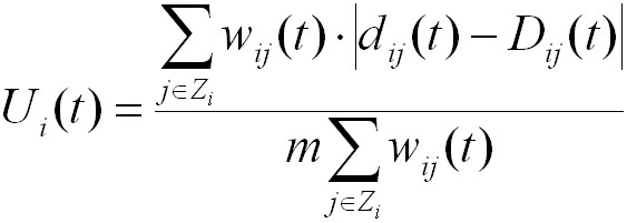
where Zi is the subset of agents perceived at time t by agent i and from which agent i keeps non-neutral ideal distances; m is the maximum possible real distance, given the dimensions of the room, and is used to rank dissatisfaction between 0 and 1; wij(t) weighs the discrepancy between the real and ideal distance; dij(t) is the current real distance between agents i and j at time t; and Dij(t) is the ideal distance agent i wants to keep from agent j at time t (for details, see Quera, Beltran, Solanas, Salafranca, & Herrando 2000).

2.2
The ideal distance agent i wants to keep from agent j can vary in accordance with some rules (or functions) that are applied whenever a behavioral event or combination of events occurs during the interaction. For the purposes of this paper, we used a function that generated ideal distances between agents as a consequence of changes in their personal and social spaces. We defined the personal (Pij(t)) and social (Sij(t)) distances of agent i with respect to agent j at time t as the lower and upper limits, respectively, for the ideal distance agent i wanted to keep from agent j at time t. Personal and social distances were the diameters of two concentric circles whose center was agent i's current location. In accordance with our model, the ideal distance varied as a function of both the personal and social distances, which changed as a function of real distance, which in turn was ultimately determined by the agent's dissatisfaction (Ui(t)).

2.3
Initially, Pij(0) and Sij(0) were assigned specific values: Pij(0) was equal to the diameter of the agent's neighborhood; and Sij(0) was equal to 3Pij(0) because, according to proxemics, the social-space distance is approximately three times greater than the personal-space distance (Hall 1966). As the simulation progressed (t = 1, 2, …) and while dij(t) > Sij(0), agent i's movements were not a product of its real distance from agent j, and Pij(t) and Sij(t) kept their initial values. During this period the agent moved randomly. The first time its real distance from agent j reached a value that was lower than or equal to its social distance from that agent, i.e., dij(t) ≤ Sij(0), the ideal distance that agent i wanted to keep from agent j changed to one of the following values: (a) if the real distance was less than the personal distance, i.e., dij(t) ≤ Pij(t), then the ideal distance was set equal to the personal distance, Dij(t) = Pij(t); or (b) if the real distance was greater than the social distance, i.e., dij(t) > Sij(t), then the ideal distance was set equal to the social distance Dij(t) = Sij(t); or (c) if the real distance was between the personal and social distances, i.e., Pij(t) < dij(t) ≤ Sij(t), then the ideal distance was set equal to the real distance, Dij(t) = dij(t).

2.4
Three different time counters were updated when each of these conditions occurred: tp, tm and ts, which were cumulative times for conditions (a), (b), and (c), respectively. Pij and Sij were also updated depending on which condition applied, and as a function of the corresponding time-counter value, provided it was greater than the given critical adaptation time T. When condition (a) applied, i.e., when the real distance was less than the personal distance, the personal distance was updated in accordance with the following formula:

Pij(t+1) = Pij(t) + r·k·T2/tp (2)

2.5
If tp = n·T (n = 1, 2, …), r = -1; otherwise r = +1. Parameter k was equal to a non-null value that was less than the neighborhood diameter. Thus, while agent j was at a distance of less than Pij(t), agent i reacted by increasing that personal distance by small amounts, and subsequently made its ideal distance with respect to agent j equal to its personal distance. In other words, agent i reacted to agent j's approaches by trying to avoid agent j, because agent i perceived agent j as an invader of its personal space. However, as the cumulative time at a specific personal distance increased and reached values equal to T, 2·T, 3·T, etc., agent i became progressively more used to agent j being at that distance, and decreased its personal distance with respect to agent j; as a result, its ideal distance from agent j decreased as well. In other words, agent i could not run away from agent j and adapted to the new situation. Subsequent increases and decreases in personal distance became progressively smaller, and therefore that distance tended towards equilibrium.

2.6
When condition (b) applied, i.e., when the real distance was greater than the social distance, the social distance was updated in the following way:

Sij(t+1) = Sij(t) + r·k·T2/tm (3)

2.7
If tm = n·T (n = 1, 2, …), r = +1; otherwise, r = -1. While agent j was at a distance from agent i that was greater than agent i's social distance with respect to agent j, agent i reacted by decreasing that social distance by small amounts, and making its ideal distance equal to its social distance. In other words, it reacted to non-approaches from agent j by trying to approach it. Still, as tm increased and reached values equal to T, 2·T, 3·T, etc., agent i became progressively more tired of agent j being at that distance, and increased its social distance substantially; as a result, its ideal distance increased as well. As subsequent changes became progressively smaller, the social distance tended towards equilibrium.

2.8
Finally, when condition (c) applied, i.e., when the real distance was greater than the personal distance and less than the social distance, these distances were updated as follows:

Pij(t+1) = Pij(t) + r·k·T2/ts Sij(t+1) = Sij(t) + r·k·T2/ts (4)

2.9
If ts = n·T (n = 1, 2, …), r = -1; otherwise, r = +1. In other words, agent i reacted by increasing both its personal and social distances by small amounts; therefore, agent i responded to an almost steady situation by trying to avoid agent j. However, as ts increased and reached values equal to T, 2·T, 3·T, etc., agent i became progressively more used to the situation and decreased both its personal and social distances with respect to agent j; consequently, its ideal distance decreased as well. As before, subsequent increases and decreases in personal and social distances became progressively smaller.

2.10
In this paper, we will systematically explore how the agents' personal and social distances evolved, depending on different parameter values (k and T) of the function that generated the ideal distances Dij, as described above.

* Method

3.1
The MD model was implemented as an agent-based computer program called P-Space written in Borland C language (Quera, Beltran, Solanas, Salafranca, & Herrando 2000; Quera, Solanas, Salafranca, Beltran, & Herrando 2000) in accordance with the following assumptions: (a) agents move in a lattice, called a room, occupying one cell at a time (i.e., time and space are measured in discrete units); (b) a cell cannot be occupied by two or more agents simultaneously; (c) at each time unit, agents decide to move within their respective neighborhoods simultaneously; and (d) agents make their decisions independently from the other agents. Figure 1 shows the interface screen of P-Space. The software and the user manual can be downloaded from http://www.ub.es/comporta/gcai/Paginas/gcai_Downloads.htm.

Figure 1
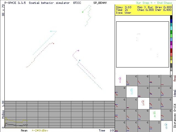
Figure 1. Interface screen of P-Space. A room with five agents is shown in the upper left section. The lower left plot shows the agents' dissatisfactions as a function of time. Ideal and real distances between agents as a function of time are shown in the lower right 5 × 5 grid. The upper right section of the screen displays the room to scale, where frequency of occupation is represented using color codes in a real screen. Also, different colors are used for identifying agents and their trajectories.

3.2
Agents have individual features: (a) initial orientation or heading, subsequent headings being defined by the direction of the agent's movement from time t to time t+1; (b) attention scope, a circular sector which is defined as an area within the room to which the agent "pays attention" at time t, so that only other agents within that area are considered when the agent computes its dissatisfaction at that time; (c) initial position within the room; and (d) the diameter and type of neighborhood, which are the same for all agents in a given simulation.

3.3
The general procedure for the simulations was as follows: First, the diameter of the neighborhood was set at 3 cells, making initial values for personal and social distances 3 and 9, respectively. Some preliminary simulations showed that the size of the room, the attention scope, and the type of neighborhood yielded no effects on Dij, so in all the simulations these parameters were assigned constant values of 80 cells × 70 cells, 360º and a Moore neighborhood, respectively. The program saved values for Pij and Sij for each agent at each time unit, as well as real and ideal distances. Thus, the dynamics of Pij and Sij over time can be observed. Moreover, when the simulation was running, the computer screen showed the room and the position of the agents in the room at each time unit. The total time units of each simulation varied depending on the time needed for Pij and Sij to reach equilibrium. The procedure of the simulation as carried out by program P-Space is outlined in the pseudocode shown in Figure 2.

Figure 2
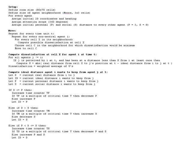
Figure 2. Pseudocode of program P-Space, indicating how ideal, personal, and social distances are updated according to changes in real distance between the agents

3.4
Two sets of simulations were carried out with P-Space: (a) a first set systematically tested the effects of critical adaptation time T and incremental parameter k on the evolution of personal and social distances; and (b) a second set of simulations tried to identify macro-level spatial-behavior patterns that might emerge as a function of parameters T and k, as well as other variables.

First set of simulations: Effects of parameters T and k

3.5
Values for parameters T and k were varied systematically in order to observe the effects on the evolution of Pij and Sij over time. Only two agents were defined: Agent 1 acted in accordance with the rules that generated ideal, personal, and social distances, while Agent 2 was immobile and neutral, i.e., it did not move and did not react to Agent 1. When the simulation started (t=0), Agents 1 and 2 were located in the center of the room, one facing the other (i.e., their headings were opposite). Agent 1's values for parameters T and k were varied using four simulation conditions obtained from previous exploratory simulations (see Table 1). P12 and S12 values were recorded during the simulation.

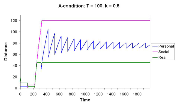
Table 1: Parameter T and k values used in the simulation

ConditionParameter T Parameter k
A1000.5
B1000.05
C100.5
D100.05

3.6
The results show that under condition A, P12 and S12 values become higher than the dimensions of the room; whereas, under conditions B, C, and D, P12, S12 and d12 reached steady values after a variable number of time units (see Figure 3). Given that D12 was equal to d12 when d12 was between P12 and S12, D12 also reached equilibrium under conditions B, C, and D. Therefore, the ideal distance agent i wanted to keep from agent j remained constant when P12 and S12 reached equilibrium. Figure 3 also shows that under conditions B and C, social distance S12 tended to be higher than under condition D (about 25 cells vs. about 8 cells). Also, under conditions C and D, personal distance P12 was lower than under condition B (about 2 cells vs. about 15 cells).

Figure 3a
Figure 3b
Figure 3c
Figure 3d
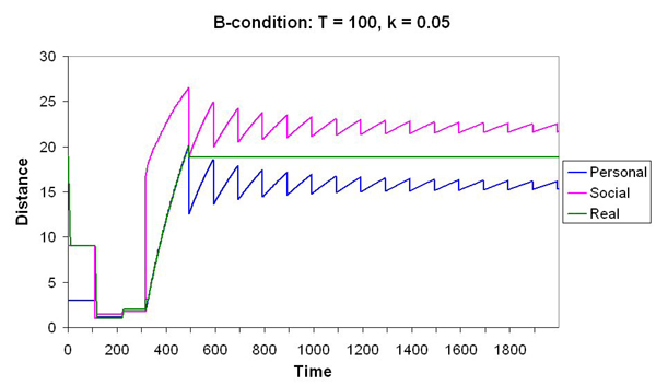
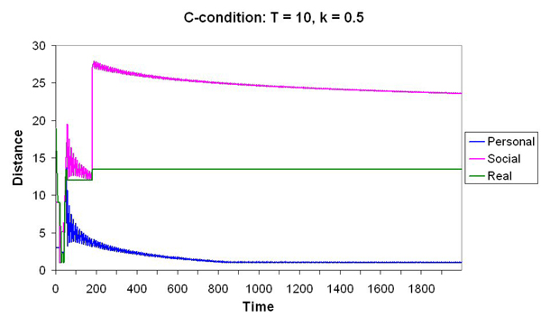
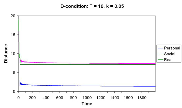
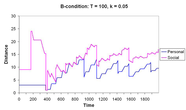
Figure 3. Evolution of personal, social, and real distances over time under simulation conditions A, B, C, and D. Distances for Agent 1 were governed by parameters T and k, which are shown in the figure. Agent 2 was immobile and neutral

3.7
A second series of simulations was carried out in order to obtain the equilibrium values for P12 and S12 when Agent 2 was neutral with respect to Agent 1, but moved randomly; the neutral agent had no ideal distances with respect to the other agent, and therefore did not experience dissatisfaction. At t=0, Agents 1 and 2 were located in the center of the room and their headings were opposite. Parameters T and k for Agent 1 were varied in accordance with the A, B, C, and D simulation conditions described above. The results are shown in Figure 4. For all conditions, P12 and S12 values were approximately the same as those found in the first simulation series, although the evolution of P12 and S12 over time was more irregular, especially under condition B.

Figure 4a
Figure 4b
Figure 4c
Figure 4d
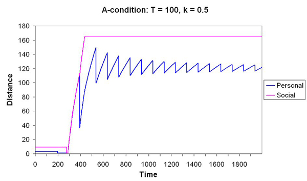
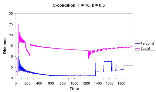
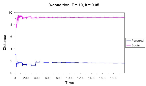
Figure 4. Evolution of personal and social distances over time for conditions A, B, C, and D. Distances for Agent 1 were governed by parameters T and k, which are shown in the figure. Agent 2 was neutral and moved randomly

3.8
Under condition B, an interesting emergent effect occurred. The perception gained from watching the computer screen while the simulation was running was that sometimes Agent 2 (which was neutral and moved randomly) was chasing Agent 1, and sometimes Agent 1 was chasing Agent 2. This behavior was obviously not the result of an order telling agents to chase each other alternately, and can be explained by Agent 1's high personal and social distance values under condition B. While moving randomly, Agent 2 invaded Agent 1's personal space, making D12 increase, which in turn prompted Agent 1's avoidance behavior; likewise, Agent 2 moved far from Agent 1's social space, making D12 decrease, which in turn prompted Agent 1's approach behavior. Thus, to an outside observer, the overall spatial dynamics of the two agents was perceived as "Agent 1 and Agent 2 are chasing each other alternately".

3.9
A third simulation series was carried out in order to determine whether the evolution patterns of personal and social distances found previously remained the same if the two agents were not neutral but acted in accordance with different values of parameters T and k. Two agents were defined: Agent 1 with T = 100 and k = 0.05 (which corresponded to condition B in the previous simulation series) and Agent 2 with T = 10 and k = 0.05 (which corresponded to condition D).

Figure 5
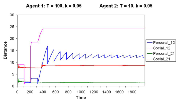
Figure 5. Evolution of personal and social distances between Agents 1 and 2 over time during the simulation

3.10
Figure 5 shows that the personal and social distances between the two agents (P12, S12, P21, and S21) tended to reach equilibrium very much like those found under conditions B and C of the previous simulation; equilibrium values were P12 = 24 and S12 = 12 (as under condition B), and P21 = 2 and S21 = 9 (as under condition C). In summary, equilibrium values of personal and social distances for a given agent were not influenced by the other agents' values for parameters T and k, and were consistent only with the agent's own T and k parameters.

3.11
In a fourth series of simulations, we compared Pij and Sij equilibrium values when the agents that interacted had identical values for T and k, and when they had different T and k values. Three agents were defined with T and k values as shown in Table 2. For instance, Agent 1 (row 1) behaved towards Agent 2 (column 2) with the parameter values corresponding to condition B (T=100 and k = 0.05), and Agent 2 (row 2) behaved towards Agent (column 1) in accordance with those same values. On the other hand, Agent 1 (row 1) behaved towards Agent 3 in accordance with the parameters of condition C (T = 10 and k = 0.5) (column 3), while Agent 3 (row 3) behaved towards Agent 1 (column 1) in accordance with the parameters of condition D (T = 10 and k = 0.05).

Table 2: Values of parameters T and k. The ideal distances for each agent (rows) towards each other agent (columns) was computed in accordance with T and k values under conditions B, C, and D (for more details, see Table 1)

Agent
123
Agent1-BC
2B-C
3DB-

3.12
The results show that Pij and Sij equilibrium values were as expected for all conditions (B, C, and D), regardless of the fact that T and k were identical or different for the two specific agents that interacted. When Agent 1 interacted with Agent 2, P12 and S12 had the same equilibrium values as those corresponding to condition B; the same occurred when Agent 2 interacted with Agent 1. Furthermore, when Agent 1 interacted with Agent 3, Agent 1's personal and social distances reached equilibrium values identical to those corresponding to condition C, whereas when Agent 3 interacted with Agent 1, Agent 3's personal and social distances reached values like those for condition D.

3.13
In conclusion, when equilibrium was reached, the agents' personal, social, and ideal distances depended on their own values for parameters T and k, which defined a trend for that agent. Furthermore, an emergent behavior that was observed under one of the conditions in the second simulation series, i.e., an agent with T=100 and k=0.05 plus a neutral agent, can be explained by the trend of the first agent.

Second set of simulations: Macro-level spatial behavior

3.14
We explored the agents' macro-level spatial behavior as a function of their parameter values while paying special attention to emergent group phenomena. To that end, we carried out a first simulation series with from 3 to 20 agents with the parameter values for conditions B, C, and D corresponding to those of the previous set of simulations. The results again show that the personal and social distances for each individual agent at equilibrium agreed with those anticipated in accordance with the agent's trend, i.e., the characteristic pattern values of personal and social distances were the same under the different conditions as those obtained in the first set of simulations. Agents behaving in accordance with the parameter values of condition B developed greater personal distances than the other agents, which produced avoidance behavior in the agents behaving in accordance with condition-B parameter values; conversely, agents behaving in accordance with the parameter values of conditions C and D developed smaller personal distances and thus tended to remain closer to the other agents. These different global patterns were very clear to an observer looking at the computer screen while the simulations were running.

3.15
Moreover, the results of the first series of simulations showed that the mobility of the group (i.e., the number of time units during which the agents were moving around the room before the group reached equilibrium) was influenced by the length of time the agents remained neutral before interaction started. According to our model, in the beginning, an agent (i) remained neutral until it encountered another agent (j), i.e., when dij(t) ≤ Sij(0) for the first time; therefore, agents did not interact during a variable number of time units after the simulation started. If an agent's first encounter was delayed with respect to the first encounter of the other agents, the first agent's time counter was different from the other agents', making it take longer for the group to reach equilibrium. As a result, the overall dynamics observed on the computer screen was of greater group mobility. Moreover, delayed agents moved randomly during the first time units of the simulation, while the other agents did not. Therefore, the delayed agents tended to invade the other agents' personal space, which produced two kinds of behavior: avoidance (as observed in the emergent chase behavior in the second simulation) or approach (when the delayed agents left the other agents' social space, which provoked approaching behavior in the other agents). This process delayed overall equilibrium. Finally, we also found that the greater the number of agents making up the group, the faster the agents reached equilibrium.

3.16
In a second series of simulations, we focused on the effects of the T and k parameters on the mobility of the group. We defined a group of four agents, two of which behaved in accordance with the parameter values of condition B (Agent 1 and Agent 2) and the other two in accordance with the parameter values of condition C (Agent 3 and Agent 4), and then observed the number of time units the agents moved around the room before the group reached equilibrium. More simulations were carried out varying the agents' parameters, which we found produced variations in the group's mobility: (a) when the T parameter was changed from T=100 to T=10 for Agent 1, Agent 2 or both of them, overall mobility decreased; (b) when the T parameter was changed from T=10 to T=100 for Agent 3, Agent 4 or for both of them, overall mobility increased; (c) when all the agents were assigned the values k=0.05 and T = 80, 100, 120, and 140, overall mobility increased as T increased. Hence, overall mobility clearly depended on the values of parameters T and k.

3.17
In summary, in the second set of simulations we observed that the parameters of the agents, i.e., the trend of each agent with respect to the other agents, determined the group's observed dynamics at the macro-level behavior, and provoked the emergence of avoidance and approach behaviors. Also, the group's mobility increased the longer the agents remained neutral during the early time units of the simulation. Mobility also increased the higher the values of parameters T and k, and when the number of agents was lowered.

3.18
Moreover, compared with the first set of simulations (in which only two agents were present), more complex group behavior was observed when a larger group of agents was defined; their global behavior, as observed on the computer screen while the simulation was running, was more diverse, as each agent reacted to several agents at the same time.

* Conclusions

4.1
The main objective of this paper was to demonstrate that our model could be used to explain the behavior observed in a group of people interacting in a closed space (such as a cocktail party), based on dyadic and local interactions using a bottom-up approach. We have briefly discussed the minimum-dissatisfaction model (MD) and used it to define the dynamics of the spatial behavior of the group. In our simulations, we explored the effects of the critical adaptation time (T) and the incremental parameter (k) on the function generating Dij and, based on that, we observed the dynamics of the macro-level spatial behavior. The two sets of simulation results show that several agents interacting with the function generating Dij in the MD model leads to the emergence of unexpected overall behavior similar to that of a group of individuals in a closed space. As discussed in the introduction, this behavior can be described but not explained from a macro-level point of view, i.e., no general rules can be stated using a classic top-down approach. In this paper, we show that it is more advantageous to describe spatial processes using a bottom-up approach, and to define the spatial behavior in a closed room as an emergent process resulting from the function governing the evolution of the personal space of each agent at the micro level.


* Notes

1 An observed global phenomenon is called emergent when it arises from the nonlinear parallel interactions of a larger set of simpler elements. For a definition of emergence, see Darley (1994).


* Acknowledgements

This project was supported by grants from the Directorate General for Research of the Government of Catalonia (2001SGR-00140) and the Directorate General for Higher Education and Culture of the Spanish Government (BSO 2001-2844). This research project also received funding from the European Union's FEDER program.

* References

CASSIDY T (1997) Environmental psychology. Behavior and experience in context. Hove, East Sussex, UK: Psychology Press.

DARLEY V (1994) "Emergent phenomena and complexity". In Brooks R A and Maes P (Eds.) Artificial Life IV: Proceedings of the fourth international workshop on the synthesis and simulation of the living systems, Cambridge, Massachusetts: MIT Press.

HALL E T (1966) The hidden dimension. Garden City, New York: Doubleday.

HAYDUK L A (1983) Personal space: Where we now stand. Psychological Bulletin, 94 (82). pp. 293-335.

HEGSELMANN R (1996) "Understanding social dynamics: The cellular automata approach". In Troitzsch, K G, Mueller U, Gilbert G N and Doran, J E (Eds.) Social science simulation, Berlin: Springer (pp. 282-306).

HEGSELMANN R and Flache A (1998) Understanding complex social dynamics: A plea for cellular automata based modelling. Journal of Artificial Societies and Social Simulation [on line], 1 (3). Available: https://www.jasss.org/1/3/1.html.

NOWAK A, Szamrej J and Latané B (1990) From private attitude to public opinion: A dynamic theory of social impact. Psychological Review, 97 (3). pp. 362-376.

QUERA V, Beltran F S, Solanas A, Salafranca L and Herrando S (2000) "A dynamic model for inter-agent distances". In Meyer J A, Berthoz A, Floreano D, Roitblat H L and Wilson S W (Eds.) From animals to animats (Vol. 6. Supplement), Honolulu: The International Society for Adaptive Behavior (pp. 304-313).

QUERA V, Solanas A, Salafranca L, Beltran F S and Herrando S (2000) P-SPACE: A program for simulating spatial behavior in small groups. Behavior Research Methods, Instruments, and Computers, 32 (1). pp. 191-196.

SAKODA J M (1971) The checkerboard model of social interaction. Journal of Mathematical Sociology, 1. pp. 119-132.

SCHELLING T (1969) Models of segregation. American Economic Review, 59, 488-493.

SCHRECKENBERG M and Sharma S D (Eds.) (2002) Pedestrian and evacuation dynamics. New York: Springer.

----

ButtonReturn to Contents of this issue

© Copyright Journal of Artificial Societies and Social Simulation, [2006]