
Alison Heppenstall, Andrew Evans and Mark Birkin (2006)
Using Hybrid Agent-Based Systems to Model Spatially-Influenced Retail Markets
Journal of Artificial Societies and Social Simulation
vol. 9, no. 3
<https://www.jasss.org/9/3/2.html>
For information about citing this article, click here
Received: 23-May-2005 Accepted: 20-May-2006 Published: 30-Jun-2006

 Abstract
|
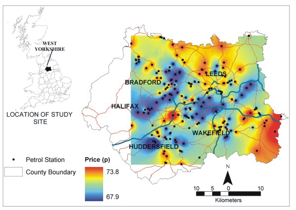
| Figure 1. Map showing the location and spatial variability of retail petrol prices within West Yorkshire. Urban areas are indicated by station density and by name |
|
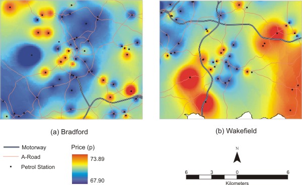
| Figure 2. Intra-urban price variation for two typical cities |
| Table 1: List of agent characteristics | |
| Characteristic | Explanation |
| Autonomous | React to other petrol agents on basis of individual and local information. |
| Heterogeneous | Stations can have individual rule sets, price and profit levels. |
| Communicative and Cooperative | Pricing and location information shared between agents for competition. |
| Pro-active | Monitor their own profit/price levels and take action to maintain or maximise their profit. |
| Reactive | Decision making on pricing rules and updating of prices based on information supplied to them. |
|
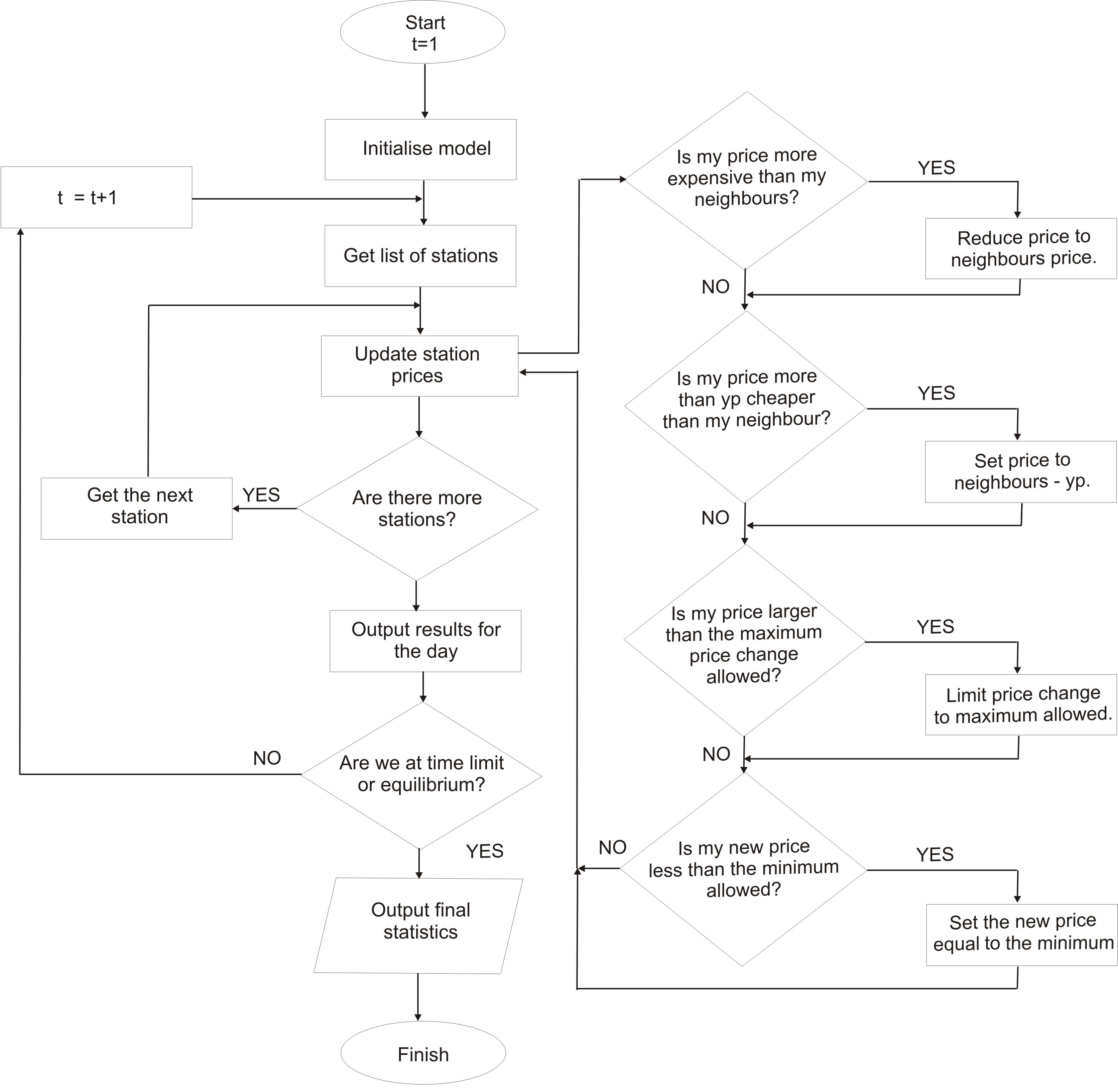
| Figure 3. Flowchart illustrating the operation of rules within the petrol agent during one iteration. For the values of parameters like "maximum price change allowed, see Appendix 2 |
|
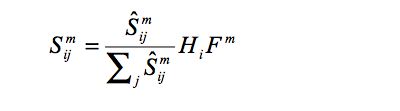
(1) |
|
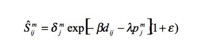
(2) |
where:
Smij is the amount of fuel m sold by garage j to ward i.The stochastic term in the calculation of the weighted distribution of sales allows for the representation of imperfect knowledge and non-rational behaviour in customers and for the addition of a random perturbation to the model. For the purposes of this paper ε is taken as being normally distributed with a mean of 0.0 pence and a standard deviation of 0.05 pence.
δmj is 1 where garage j sells fuel m and 0 otherwise.
dij is the distance between ward i and garage j.
pmjis the price of fuel m at garage j.
Hi is the number of households within the ward i.
Fm is the amount of fuel of type m required per car per day.
ε is a stochastic term.
|
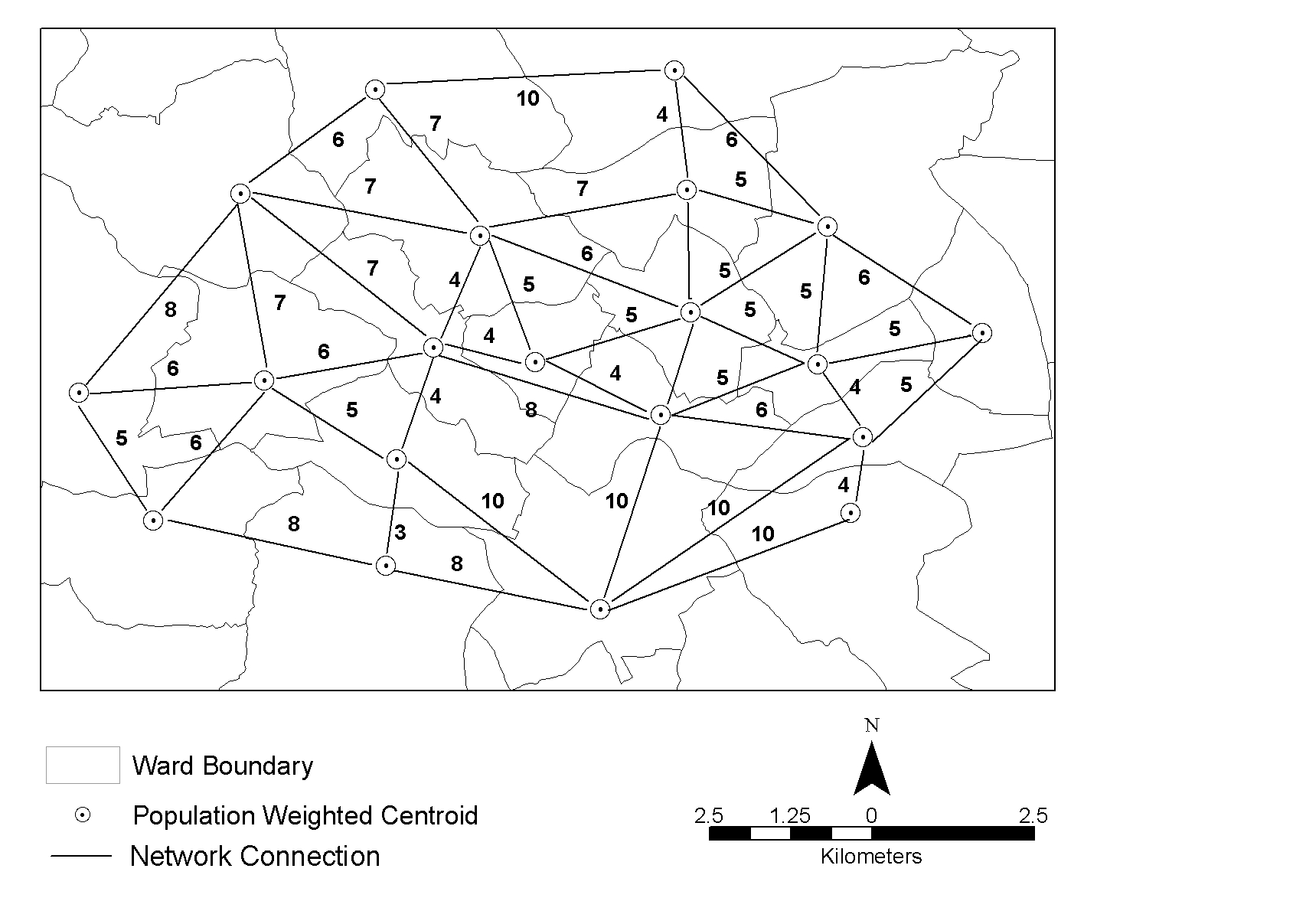
| Figure 4. A section of the weighted graph network |
|
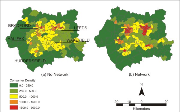
| Figure 5. Distribution of consumer density before (a) and after (b) application of the networking |
| Table 2: Comparison of the Hybrid and Network models running the models in deterministic and stochastic mode. The model was run ten times in stochastic mode to generate the ranges. The first and second rows are the mean and standard deviation of the errors between the real and predicted data | |||||
| Test | Hybrid-Model | Network-Model | |||
| Business as usual | Deterministic | Stochastic | Deterministic | Stochastic | |
| Mean | 0.160 | 0.138 | 0.137 — 0.143 | 0.152 | 0.149 — 0.155 |
| SD | 0.976 | 1.007 | 1.004 — 1.012 | 1.037 | 1.036 — 1.044 |
| RMSE | 0.987 | 1.018 | 1.012 — 1.019 | 1.046 | 1.044 — 1.054 |
| MAE | 0.773 | 0.783 | 0.781 — 0.788 | 0.806 | 0.805 — 0.814 |
|
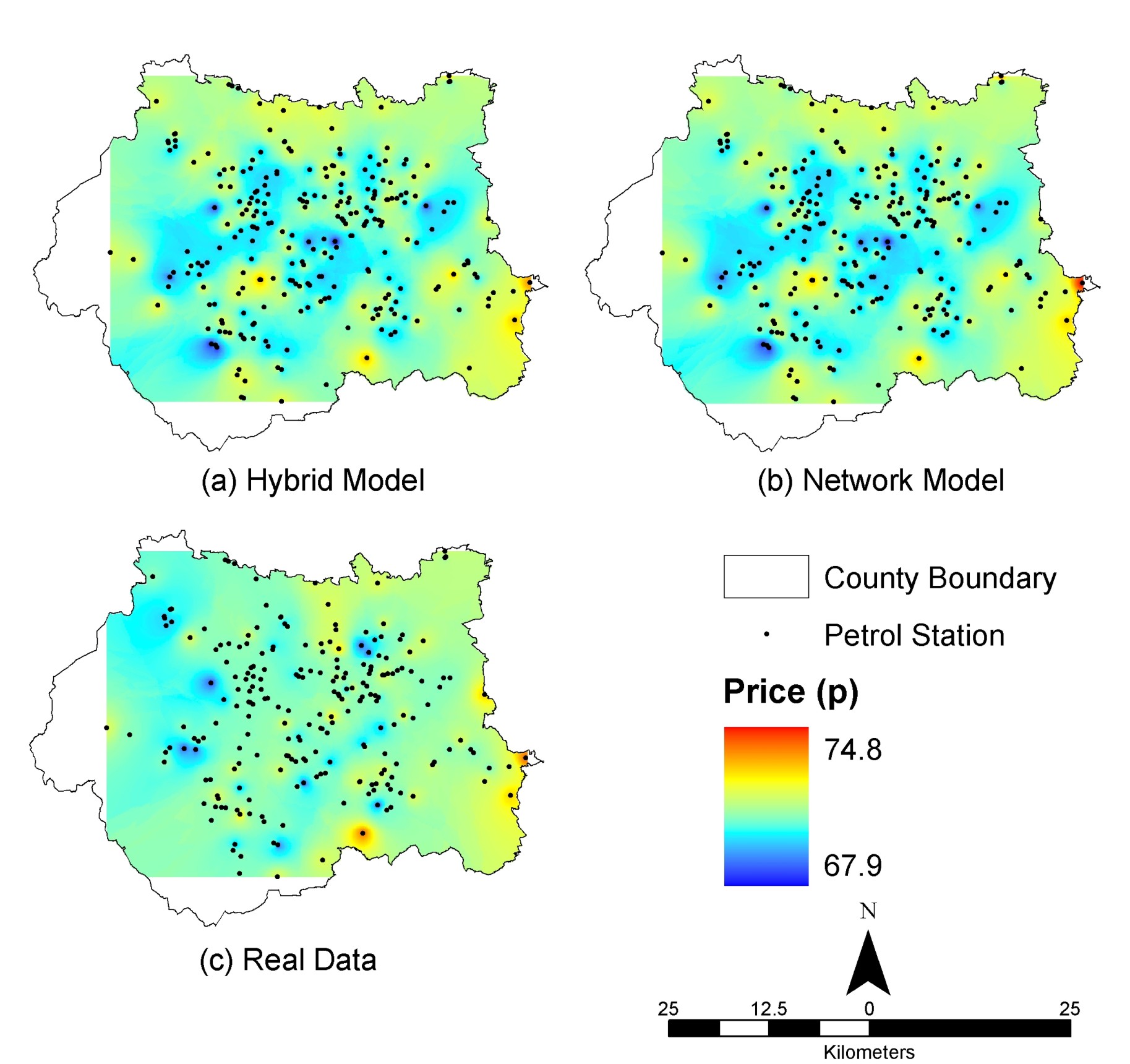
| Figure 6. Price distributions for the various models ten days after runs started with all stations initialised at 71p: (a) Hybrid-model and (b) Network-model. Data from day ten of the real data set (c) is included for comparison |
| Table 3: Aggregated results of running the model with a random price drop and increase of 1p and 3p at random stations. Each experiment was run ten times. The first and second rows are the mean and standard deviation of the errors between the real and predicted data | |||||
| Test | Price Drop | Price Increase | |||
| Real Data | 1p | 3p | 1p | 3p | |
| Mean | 0.160 | 0.183 — 0.196 | 0.199 — 0.777 | 0.177 — 0.203 | 0.179 — 0.200 |
| SD | 0.976 | 1.018 — 1.043 | 1.031 — 1.590 | 1.012 — 1.038 | 1.027 — 1.058 |
| RMSE | 0.987 | 1.033 — 1.058 | 1.048 — 1.767 | 1.026 — 1.056 | 1.042 — 1.078 |
| MAE | 0.773 | 0.788 — 0.803 | 0.798 — 1.271 | 0.786 — 0.801 | 0.786 — 0.810 |
|
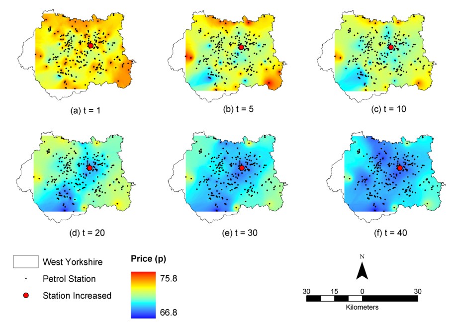
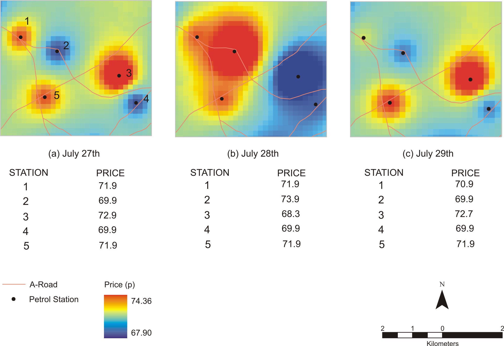
| Figure 7. Spatial diffusion of prices over time for a price drop of 5 pence. All stations are initialised with real prices from day zero (July 27 th) |
|
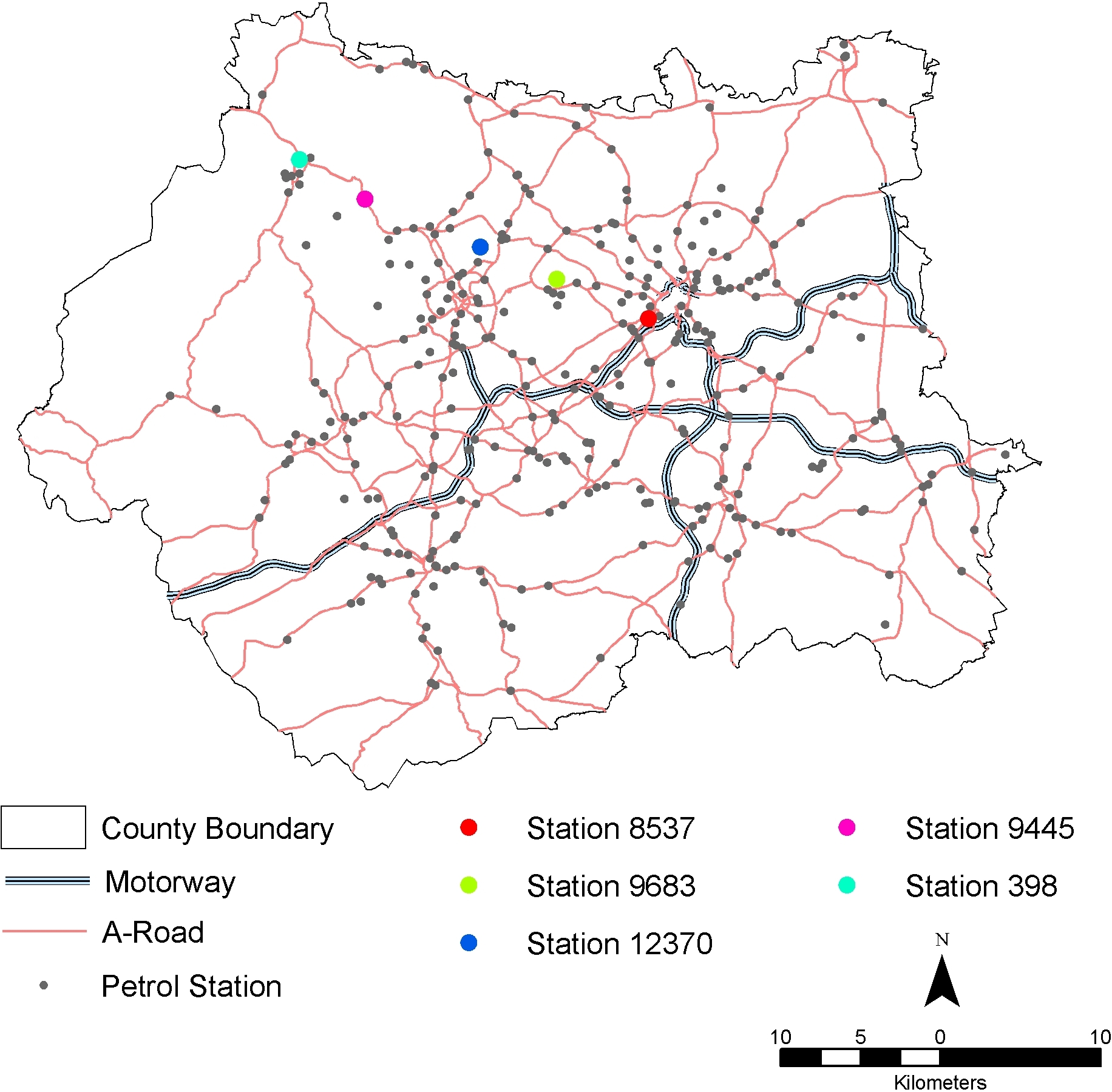
| Figure 8. Location of stations examined in the experiments |
|
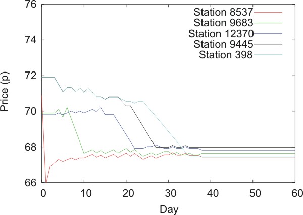
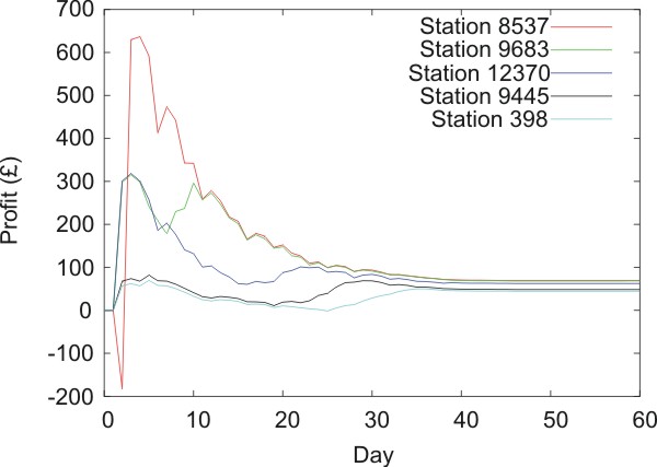
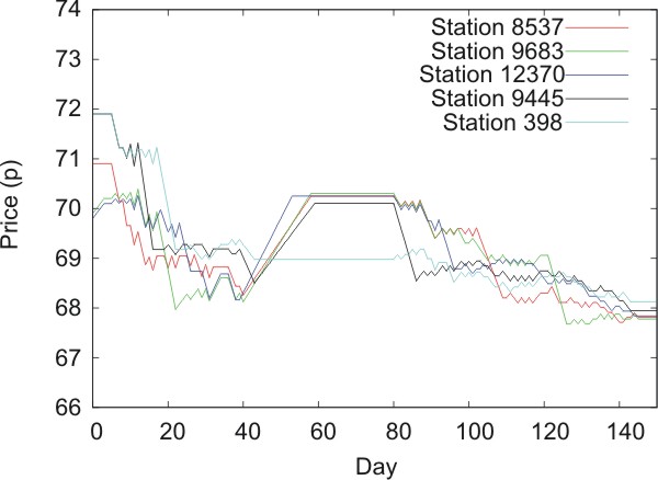
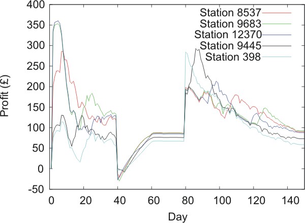
| Figure 9. Change in (a) price and (b) profit over time for the selected stations in the real data diffusion experiment with a price drop of 5 pence |
|
| Figure 10. Mean price (a) and profit (b) plotted against time for simulations of the "rockets and feathers" effect using the West Yorkshire data |
|
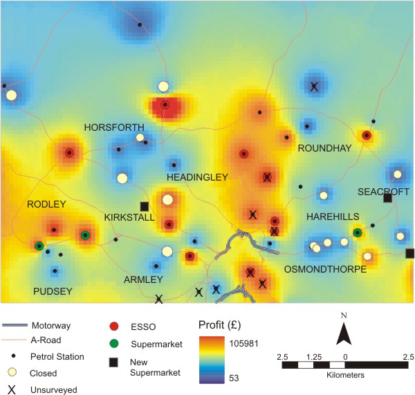
| Figure 11. Map showing the profitability of stations in Leeds using the Network-model with data from 1999. Also shown for comparison are the status (open or closed) of the stations in 2004 |
| Table A1: Parameters | |
| Parameter | Definition |
| B | Coefficient controlling the impact of distance. |
| λ | Coefficient controlling the impact of price. |
| fixedCosts (£) | The amount the petrol station has to pay per day to keep running. |
| costToProduce (p) | The amount per litre that it costs the station to produce and sell the petrol. |
| changeInProfit (p) | The level of profit under which the station will not change its strategy. |
| Overprice (p) | The amount by which petrol stations can be more expensive than their neighbours without becoming uncompetitive and being forced to cut their price. |
| Undercut (p) | The amount by which petrol stations can undercut competitors, e.g. 1p, 2p. |
| Neighbourhood (km) | The distance that the petrol stations will treat as their neighbourhood e.g. 2km, 3km. |
| Table A2: Experiment parameter values | |
| Parameter | Value |
| B | 0.0003 |
| λ | 0.7 |
| fixedCosts (£) | 80.00 |
| costToProduce (p) | 66.00 |
| changeInProfit (p) | 40.00 |
| Overprice (p) | 5 |
| Undercut (p) | 1 |
| Neighbourhood (km) | 5.0 |
|
| Figure A1. |
BACON, R.W. (1991). Rockets and Feathers: the Asymmetrical Speed of Adjustment of UK Retail Gasoline Prices to Cost Changes. Energy Econ, 1:211 - 218.
BIRKIN, M., CLARKE, G., CLARKE, M. AND WILSON A. (1996). Intelligent GIS: Location decisions and strategic planning. GeoInformation InternationalBIRKIN, M., CLARKE, G. AND CLARKE, M. P. (2002). Retail Geography and Intelligent Network Planning. Wiley, 1st edn.
BRUNSDON, C., FOTHERINGHAM, A. S. AND CHARLTON, M. E. (1998a). Geographically Weighted Regression - Modelling Spatial Non-Stationarity. Journal of the Royal Statistical Society - Series D - The Statistician, 47(3): pp431 - 443.
BRUNSDON, C., FOTHERINGHAM, A. S. AND CHARLTON, M. E. (1998b). Spatial Non-Stationarity and Autoregressive Models. Environment and Planning A, 30(6): pp957-993.
BUNN, D. W., and OLIVERIA, F. S. (2001). Agent-based simulation: An application to the New Electricity Trading Arrangements of England and Wales. IEEE Transactions on Evolutionary Computation (5): pp493-503.
CASTIGLIONE, F. (2000) Diffusion and aggregation in an agent based model of stock market fluctuations. International Journal of Modern Physics C 11 (5): 865 - 879.
COMPETITION COMMISSION (1990). Petrol Pricing. URL http://www.competition-commission.org.uk/rep_pub/reports/1990/fulltext/265c4.pdf.
CONSTANTINIDES, E. (2002). Influencing the online consumer's behaviour: the Web Experience. Internet Research-Electronic Networking Applications and Policy 14(2) pp 111 - 126.EMCAS, Electricity Market Complex Adaptive Systems. Argonne National Laboratory. http://www.dis.anl.gov/ceeesa/programs/emcas.html. Accessed May 2006.
GALOETTI, M., LANZA, A. AND MANERA, M. (2003) "Rockets and Feathers Revisited: An International Comparison on European Gasoline Markets". Energy Economics, 25 pp175-190.
GARCIA-FLORES, R. AND WANG, X.Z. AND GOLTZ, G.E. (2000). Agent-based Information Flow for Process Industries' Supply Chain Modelling. Computers and Chemical Engineering 24(2-7) pp1135 - 1141.
HA, S.H., BAE, S.M. and PARK, S.C. (2002). Customer's Time-Variant Purchase Behaviour and Corresponding Marketing Strategies: An Online Retailer's Case. Computers and Industrial Engineering. 43(4) pp801 - 820.
HEPPENSTALL, A.J. (2004) Application of Hybrid Intelligent Agents to Modelling a Dynamic, Locally Interacting Retail Market. Unpublished Thesis. School of Geography, University of Leeds.
HEPPENSTALL, A.J., EVANS, A.J. AND BIRKIN, M.H. (2005). A Hybrid Multi-Agent/Spatial Interaction Model System for Petrol Price Setting. Transactions in GIS 9(1) pp 35 - 51.
HEPPENSTALL, A.J., EVANS, A.J. AND BIRKIN, M.H. (2006), Genetic Algorithm Optimisation of a Multi-Agent System for Simulating a Retail Market. In press, Environment and Planning B.
JULKA, N. AND SRINIVASEN, R. and KARIMI, I. (2002). Agent-based supply chain Management-1: Framework. Computers and Chemical Engineering. 26(12) pp 1755- 1769.
KIRMAN, A., AND VRIEND, N. J. (2001). Evolving Market Structure: An ACE Model of Price Dispersion and Loyalty. Journal of Economic Dynamics and Control 25, pp 459-502.
LOMBARDO, S., PETRI, M., and ZOTTA, D. (2004). Intelligent Gis and retail location dynamics: A multi agent system integrated with ArcGis. Computational Science And Its Applications - Iccsa 2004, Pt 2 Lecture Notes In Computer Science, 3044: 1046 - 1056.
MANNING, D. N. (1991). Petrol Prices, Oil Price Rises and Oil Price Falls: Evidence for the UK since 1972. Applied Economics, 23:1535 - 1541.
MITCHELL, J. D., Ong, L. L. and Izan, H. Y. (2000). Idiosyncrasies in Australian Petrol Price Behaviour: Evidence of Seasonalities. Energy Economics, 28:243 - 258.
NING, X. AND HAINING, R. (2003). Spatial Pricing in Interdependent Markets: A Case Study of Petrol Retailing in Sheffield. Environment and Planning A, 35:2131 - 2159.O'SULLIVAN, D. AND HAKLAY, D. (2000). Agent-based Models and Individualism: Is the World Agent-Based? Environment and Planning A, 32(8) pp1409 - 1425.
PETTERSEN, E., PHILPOTT, A.B. AND WALLACE, S.W. (2005). An Electricity Market Game Between Consumers, Retailers and Network Operators. Decision Support Systems, 40(3-4) pp427 - 438.
PLUMMER, P. S., SHEPPARD, E. AND HAINING, R. P. (1998). Modeling Spatial Price Competition: Marxian versus Neoclassical Approaches. Annals of the American Association of Geographers, 88(4): pp575 - 594.
PONTIUS, R.G. Jr, HUFFAKER, D., and Denman, K. (2004). Useful Techniques of Validation for Spatially Explicit Land-Change Models. Ecological Modelling, 179: 445 - 461.
REILLY, B. AND WITT, R. (1998), "Petrol Price Asymmetries Revisited", Energy Economics, 20 pp297 - 308.
SHIN, D. (1994). Do Petrol Prices Respond Symmetrically to changes in crude oil prices? OPEC Review, 18:137 - 157.
SIGNORILE, R. (2002). Simulation of a Multi-Agent System for Retail Inventory Control: A Case-Study. Simulation-Transactions of the Society for Modelling and Simulation International 78 (5) pp 304 - 11.
 Return to Contents of this issue
© Copyright Journal of Artificial Societies and Social Simulation, [2006]