Anselm Fleischmann (2005)

A Model for a Simple Luhmann Economy

Journal of Artificial Societies and Social Simulation vol. 8, no. 2
<https://www.jasss.org/8/2/4.html>

To cite articles published in the Journal of Artificial Societies and Social Simulation, reference the above information and include paragraph numbers if necessary

Received: 20-Sep-2004    Accepted: 28-Feb-2005    Published: 31-Mar-2005

Abstract

The core of this work is the definition of an agent-based model for a simple Luhmann economy based on publications of Niklas Luhmann. Using an implementation on a default personal computer the behaviour of the model is studied when assumptions regarding initial conditions are made. Fuzzy-c-means clustering is used as visualisation aid. The impact of the observation horizon (a model parameter determining how far agents can see) is studied interactively. Solution paths of the Luhmann economy originating from an initial endowment to equilibrium (when the economy settles down) are studied. The impact of model parameters determining the unevenness regarding the initial distribution of wealth is studied by Monte Carlo simulation. Niklas Luhmann's hypothesis, that the economy starts from and produces further inequality in order to continue (see Luhmann 1988, p. 112) could be reproduced by computer simulation. The main characteristic of the approach is the consideration of the cohesive structure of communication (i.e. one communicative act - many understanding observers) also prominent in Dunbar (1996, pp. 192-207). The model gives directions how to model further aspects of Niklas Luhmann's theory.

Keywords:

Agent-Based Modelling, Luhmann Economy, Fuzzy Clustering

Introduction

1.1

Niklas Luhmann's social theory uses many abstract concepts but is not formulated in a formal language. It has become an important line of thought within sociology (Joas and Knöbl 2004, pp. 351-392) but it is hard to access for other disciplines. Several attempts have been made to formalise Niklas Luhmann's work by the usage of agent-based models. Most prominent are models focussing on the emergence of symbols^[1] (see Kron and Dittrich 2002) as well as models that emphasise the anticipation/recursion dichotomy^[2] (see Leydesdorff 2004).

1.2

As economic concepts such as the exchange of goods between agents are easier to capture in quantitative terms, this paper tries to model along Niklas Luhmann's publication about the economy (Luhmann 1988). It describes an agent-based model for a simple Luhmann economy. The term simple Luhmann economy and the assumptions used for an agent-based model are explained in the next sections.

1.3

Once a model for a Luhmann economy is developed, it may serve as a template for other function systems^[3] (e.g. law, politics, family). Models may even be combined to study mutual effects. Nelson and Winter (1982, p. 405) comment on the linguistic and conceptual isolation of economics and its sister social sciences. Choosing Luhmann (1988) as a template for modelling may help to bridge this gap.

Luhmann Economy

1.4

Luhmann (1988) contains an analysis of economic phenomena - or rather economic communications - on the proposition that the function system^[4] economy is one of several subsystems of society^[5]. Evolutionary arguments^[6] are used to explain the historical development to the present, thus leading to the following stages of economic development (simplified and summarised):

• Stage 1: Scarcity and the Ownership-code

  In order to secure future access to a finite set of goods, people provisionally access (store, own) these goods. Access as a solution to the problem of scarcity creates further scarcity. This is referred to as the scarcity paradox. The ownership code (to own or not to own) gets established. To own something (desirable) is better that not owning it. The code is asymmetrical.

• Stage 2: Money, the Money-code and the Double cycle

  The money-code (to pay or not to pay) superimposes the ownership-code when the usage of money becomes established. It is not necessarily better to pay than not to pay (or vice versa). This code is symmetrical. Payments enable further payments. Solvability is passed into one direction. Insolvability is passed into the other direction. This is referred to as the double cycle. The economic system gains autonomy, as the value of money (interest) is determined within the economic system. Niklas Luhmann points to the similarity to meaning, because meaning is determined within the social system society^[7].

• Stage 3: Prices and Markets

  Markets are observation horizons where consumers can efficiently observe (many) other consumers, suppliers can efficiently observe many other suppliers using prices.

• Stage 4: Risks

  Dangers, attributed to events in the environment, are converted to risks, attributed to decisions in the economic system^[8].

Stage 1 is referred to as a "simple Luhmann economy" in this paper.

Modelling Implications

1.5

In order to apply the technique of agent-based modelling (Axelrod 1997)^[9], the following key concepts of Niklas Luhmann's theory of social systems were used as assumptions:

• Assumption 1: Elements of social systems are events of communications^{[10] [11] [12]} when understood
• Assumption 2: The structures of systems are made of expectations^{[13] [14]}
• Assumption 3: Communication transforms the difference of information and utterance to the difference of acceptance or rejection of the utterance^{[15] [16] [17]}
• Assumption 4: The structures of a system can only be determined by its own operations^[18]

  Remark: Psychic and social systems evolve by means of Co-evolution ^[19]

1.6

An important consequence is, that neither people (psychic systems^[20]) nor the physical world, are "part of" the social system under consideration but do belong to its (necessary) environment. This equally holds for the economic system. Communications that belong to other function systems (e.g. politics, law, science) are part of its environment.

A Model for a Simple Luhmann Economy

2.1

The following design goals were used for the model presented in this paper:

• correspond to a Luhmann economy as defined in stage 1 of the introduction;
• follow the assumptions given in the introduction, so that the model can be used as template for other social systems;
• enable a comparison of simulation results with known behaviour of classes of systems of difference equations;

2.2

The simulations should confirm Niklas Luhmann's hypothesis of the (autopoietic) propagation of inequality that drives the economic system. Agent-based models that study similar economic phenomena - without making use of Niklas Luhmann's concepts of social systems - were developed by Pingle and Tesfatsion (2003). Visualisation techniques will be used to investigate patterns of internal differentiation.

Agents and Neighbourhoods

2.3

Each agent inhabits exactly one of n * m squares. The squares are positioned in a 2-dimensional lattice (world) with n rows and m columns. Both n and m are natural numbers ≥ 1.

2.4

Agents have the ability to observe other agents that are within reach of the observation horizon o. o is a natural number and denotes how many rows or columns apart an agent can "see". So in the straight forward case when o = 1 an observing agent can observe all its eight (north, south, west, east and in between directions) neighbours and of course itself.

2.5

Edges are eliminated by closing the array like a torus, so that row 1 is also neighbouring row n, as well as column 1 is also neighbouring column m. By this the number of observable squares is the same for all agents with the same observation horizon o.

2.6

It is further assumed that all agents have the same observation horizon and behave according to the same rules.

Portfolios

2.7

There are g different goods that can be owned and traded by agents. g is a natural number ≥ 2.

2.8

Each agent has a portfolio of g different goods. An n*m × g stock matrix A_t describes the portfolios (stocks) of all agents at discrete time t ≥ 0. Because goods are modelled undividable all entries in matrix A_t are natural numbers. There is no short selling (or credit), so A_t ≥ 0 for all t.

Trades and Trade Runs

2.9

Agents trade with other agents within their observation horizon. A single trade involves two trading agents and two goods. One agent proposes to exchange an amount of good A in exchange for an amount of good B.

2.10

Let an n*m × n*m × g matrix P_t describe all the proposals from agents i to agents j regarding goods k at time t. A proposal from agent i to agent j implies exactly two entries different from zero in the ij ^th g-vector of the proposal matrix P_t. One strictly positive indicating an intended good's flow from agent i to agent j; one strictly negative in the reverse direction; all others zero. When there is no proposal from agent i to agent j the the ij ^th g-vector of matrix P_t is all zero.

2.11

The second (accepting) agent can only accept or refuse a proposal. There are no further choices. The deal matrix D_t has the same dimension as the proposal matrix P_t and describes the deals made by agents, when proposals are accepted.

2.12

Trades are always completed by both agents in the way they are agreed. No defection/cooperation type of behaviour (e.g. agents take proposed good A without exchanging good B) like an iterated prisoner's dilemma (Axelrod 1984, p. 8) is considered in the model. In a limited sense a trade is always beneficial for both partners. Agents receive at least something, comparable to solutions of the ultimatum bargaining game (Mehlmann 1997, pp.119-121).

2.13

A trade run involves the following steps:

• Agents direct proposals to other agents in their respective observation horizon. The matrix P_t is calculated following the proposal rule.
• Agents accept the (economically) best proposals among the received proposals. The matrix D_t is calculated according to the acceptance rule
• The accepted proposals (deals) are cleared. The new stock matrix A_t+1 is calculated from the old stock matrix A_t and the accepted trades D_t.

2.14

Given the definitions above, a trade run affects the stock matrix A_t without changing the total quantities of each good (the sum of owned goods is constant).

2.15

In mathematical notation this reads as follows: A_t^T* 1_n*m = w for all t. w is a g-vector denoting the total wealth of the system. 1_n*m is an n × m-vector of 1s.

Observation

2.16

The rules that define the making of proposals and the acceptance of deals depend on mutual observation of agents. Agents are modelled with the ability to distinguish between themselves and their environment. An agent's (constructed) environment is constituted by the observable behaviour of those agents located within the observation horizon of the observing agent.

2.17

Regarding itself an agent observes:

• Its own portfolio
• Its committed proposals during a trade run, to ensure that nothing is promised that cannot be fulfilled before deals are cleared.

2.18

Regarding its environment (the behaviour of other agents within the observation horizon) an agent observes:

• Showoffs of agents in its observation horizon. Showoffs are displays of an agent's wealth.
• Among the proposals only these, which are directed towards the observing agent can be observed. Proposals that other agents direct to other agents cannot be observed (even within the observation horizon).
• Accepted deals of all agents in its observation horizon.

The proposal and acceptance rules are the same for all agents.

2.19

The rules regarding observation of other agents, making decisions upon other agents' behaviour and offering communication (acting) implemented in this model are a specific choice following the idea of bounded rationality as introduced by Simon (1951).

2.20

As observation is linked to making expectations in Niklas Luhmann's theory our agents' observations, which are subject to change, correspond to the notion of cognitive expectations. Our agent's decision rules (staying the same throgout trade runs) correspond to normative expectations (Luhmann 1984, p. 437; Luhmann 1995, pp. 320, 321).

2.21

A more general setting requires choices among decision rules (function spaces). The models presented in Kron (2002, pp. 175 ff, 209 ff) make use of these concepts but implement communication as a one-to-one^[21] interaction between agents. The model presented here uses n-to-m communication patterns constrained by restrictions on mutual observaility of agents.

Displays of Wealth (Show Off)

2.22

Agents can perform displays of wealth called showoffs. Cheating, lying or misunderstandings (errors in information transfer) are not considered in the model.

2.23

As the model does not include prices or (explicit) utilities the following simple showoff rule is implemented:

• With a probability p show off quantity and identity of the most numerous good. If the good is not unique the lexicographic^[22] order is used to select good and wealth to be displayed.

2.24

To study the behaviour of the system when not influenced by other probabilities than the initial wealth of the system the showoff probability p is set to 1^[23].

2.25

There are reasonable other rules, e.g.

• Given prior exchanges of goods at observed exchange rates (memory is needed) the most valuable instead of the most numerous could be selected.
• More than one good is shown off

2.26

In terms of the mathematical description the showoff rule is a one-to-one map showoff: A → A, of the set of n*m × g (stock) matrices A into itself. Let the matrix X_t be the observable (shown off) wealth. Note that X_t ≤ A_t for all t.

Rule for Making Proposals

2.27

Every agent can direct proposals to all its neighbours. Depending on an agent's observations different rules are applied:

• The arbitrage rule is applied, when an agent observed (at least) two further agents exchanging the same goods in different quantity ratios ("prices")
• The proposal rule following showoff is applied, when no proposals can be made according to the arbitrage rule, e.g. when no deals were observed. By definition this is the case at time t = 1. One can understand the showoff rule as an activity rule in the sense that it triggers further activities. The term activity rule corresponds to the term used in auction theory (see Milgrom 2003, p. 6).

The rule for making proposals comprises two sub rules that are slightly more complicated than the general setting. They are described in the following chapters. In mathematical notation the overall proposal rule can be described as a one-to-one map propose: A × Δ × A → Δ . A denotes the set of n*m × g (stock) matrices as before. Δ denotes the set of n*m × n*m × g (proposal, deal or flow) matrices. As proposals depend on stock prior deals and displayed wealth the following identity holds P_t = propose(A_t,D_t-1,showoff(A_t)) for all t ≥ 1.

Arbitrage Rule

2.28

The main idea behind the arbitrage rule is the concept of naive prognosis, i.e. tomorrow will be the same as today. In the context of this model this means: If an agent observes another agent exchanging goods A and B in certain quantities, the agent expects the observed agent to do the same in the next run.

2.29

The situation, in which agent i makes proposals according to the arbitrage rule is characterised as follows:

• More than one exchange between two goods A and B have been observed at different quantity ratios, i.e. "prices".
• Agent i assumes by naive prognosis, that the observed agents will repeat their behaviour and are therefore likely to accept a proposal, that is at least as good as the observed deal.
• Agent i owns a sufficient disposable quantity of goods A and B respectively, so a proposal, when accepted can be fulfilled.

2.30

Without loss of generality agent i selects good A as the primary object of the intended trade and selects good B as payment. Given this distinction, the set of observed deals (exchanges between A and B) can be split up in observed purchases (of good A) and observed sales (of good A) according to the sign of the observed deal.

2.31

In this setting a purchase (of good A, say by agent j ≠ i) constitutes an opportunity to sell the same good A (at the same price) to this agent j. Following the same reasoning, a sale by agent j ≠ i constitutes an opportunity to buy. Agent i now selects the cheapest price, i.e. the quantity of good B for one piece of good A among the opportunities to buy and the highest price among the opportunities to sell. If this cheapest purchase price is lower than the highest sales price, then a proposal is addressed to each of the agents, where the respective prices have been identified. If the disposable stock admits only one proposal, only one proposal is made. If the cheapest purchase price or the highest sales price is not unique, the agent with the lexicographic^[24] smallest index is selected respectively.

2.32

Reasonable variations of this arbitrage rule could be the following:

• A higher purchase price or a lower sales price could be offered as an incentive to price out competition
• In case where prices are not unique, all "best price" agents could be addressed, as long as there is enough disposable stock.

The Arbitrage rule as outlined above was chosen as the most simple and straightforward one.

Proposal Rule following Showoff

2.34

Proposals are made according to the proposal rule following showoff, when no arbitrage rule proposals could be made. The showoff rule is less complex than the arbitrage rule. Before an agent i makes a proposal according to the showoff rule, it faces the following situation:

• other agents (within the observation horizon) gave displays of their wealth.
• From the above observations agent i computes, who is the wealthiest neighbour regarding every good.

2.35

For every good k₁ the procedure is followed:

• If agent i owns at least as much as (or 1 piece less than) the wealthiest neighbour, agent i "experiences" no scarcity, is confident and does nothing.
• If agent i owns less than 2 pieces than its wealthiest neighbour, scarcity is "experienced". Agent i now selects good k₂ ≠ k₁ as the good where it owns the highest disposable quantity.
• If such a good k₂ can be identified, agent i proposes to give 1 piece of k₂ to its wealthiest neighbour in exchange for receiving half (truncated to integer) of the difference between the neighbour's and its own wealth (of good k₁).

When the wealthiest neighbour is not unique, the neighbour with the lexicographic^[25] smallest index is selected.

2.36

Possible variations of the proposal rule following showoff include

• Less greedy behaviour by offering more than one piece of good k₂, especially if a considerable quantity of k₂ (more than the observed minimum) is owned.
• Propose to all wealthiest neighbours, if there is more than one and sufficient "payment" is available.

For simplicity reasons the show off rule as outlined above was selected in the model.

Rules for Accepting Proposals

2.37

Deals are accepted following a rule that is similar to the arbitrage rule. Before accepting deals between goods A and B agent j is in the following situation

• Zero, one or more proposals to exchange good A and B were addressed to agent j

2.38

For all suitable combinations of goods A and B agent j follows the following rule

• If no proposals are present, do nothing
• If one proposal is present, accept it if it can be fulfilled.
• If more than one proposal is present - without loss of generality - agent j selects good A as the primary object of the intended trade and selects good B as payment. Proposals are split into two distinct sets, a set of proposals to buy good A and a set of proposals to sell good A.
• Among the proposals to buy good A the minimum purchase price is selected. Among the proposals to sell good A the highest sales price is selected.
• The proposal with the lowest purchase price and the proposal with the highest sales price are accepted if the lowest purchase price is lower than the highest sales price. Each proposal is made subject to the no short selling condition.
• If one of the sets is empty (i.e. when there are either only proposals to buy or only proposals to sell) the proposals with the lowest purchase price (or in the other case the proposal with the highest sales price) are accepted, subject to the no short selling condition.

If lowest purchase prices or highest sales prices are not unique, the lexicographic^[26] order is used to determine a unique proposing agent.

2.39

The rule according to which a proposal to exchange good A with good B is accepted, if there is only one of its kind available (singleton proposal) can be considered rational for the following reasons: If the (singleton) proposal was addressed to the agent according to the arbitrage rule then a proposal with the same price was selected in an earlier run. If - in the other case - the proposal was addressed to the agent according to the proposal rule following showoffs there is no competitive argument. Still the following holds:

• Let without loss of generality A be the good that is to be purchased by agent j and good B the payment.
• In this case B must have been the good that agent j showed off in the prior round. Given the chosen showoff rule - only these goods are shown off, that are owned in largest quantities - receiving quantities of the (scarcer) good A in compensation for the (less scarce) good B cannot be ruled out as uneconomic.

2.40

Possible variations of the deal acceptance rule include

• A consideration of transitivity (only needed with more than 2 goods). An "exchange rate" of good A with good B plus an "exchange rate" of good B with good C may influence the evaluation of exchanges between A and C. For the sake of simplicity (and in the absence of money) transitivity was not considered in the model.
• Accept all best proposals, if there is more than one and the no short-selling condition can be met.
• A more elaborate strategy with singleton proposals

For the sake of simplicity the acceptance rule as outlined above was selected.

2.41

In mathematical notation the deal acceptance rule can be described as a one-to-one map deal: A × Δ → Δ using the same definitions for A and Δ as before. The acceptance of deals depends on stock and (pending) proposals and reads in functional form as follows D_t = deal(A_t,P_t) for all t ≥ 1.

2.42

As all maps showoff, propose, deal are are one-to-one they can be combined into a map trade: A × Δ → Δ , so that the (simplified) identity holds D_t = trade(A_t,D_t-1) for all t ≥ 1.

Clearing Deals

2.43

The last step of a trade run is the clearing of deals. It does not involve any action or communication of the agents. In this model, it is assumed that all agents have dealt with each other within one "tick" of time. Resetting the variables of all agents in a bookkeeping manner can therefore be done in one final, separate step. A different model architecture (e.g. picking agents at random that deal with and observe each other) would require the same clearing immediately after each deal on an individual level.

2.44

In this step the flows (deals) are added to the stock according to the straight forward rule:

ai,k,t+1 = ai,k,t + Σj di,j,k,t - Σj dj,i,k,t for all i, k and t

Given the definitions above, the clearing of deals can be expressed in matrix notation as a one-to-one map clear: A × Δ → Δ giving the identity A_t+1 = clear(A_t,D_t).

Dynamics

2.45

The dynamics of the system can be summarised by the following equalities:

Flows:	Dt = trade(At, Dt-1) = deal(At, propose(At, Dt-1, showoff(At)))
Stocks:	At+1 = clear(At, Dt).

subject to the following initial and transversality conditions:

• The initial wealth is fixed at t = 0, A₀ is fixed
• There are no prior trades to t = 1. D₀ = 0_{n*m × n*m × g}, so A₁ = A₀
• No short selling: A_t ≥ 0 and integer for all t
• The total wealth remains constant: A_t^T * 1_n*m = w for all t.

and the definitions:

• A_t element of A, A denotes the set of n*m × g finite integer matrices
• D_t element of Δ , Δ denotes the set of n*m × n*m × g finite integer matrices
• n, m, g, t elements of N₀; t ≥ 0; n, m ≥ 1; g ≥ 2

2.46

The specifics of the model are:

• There is no (explicit) utility function - the only assumption is that more (of any scarce good) is better than less. None of the goods has a special role (like money). Which good is exchanged most is determined by the model's simulation runs.
• As there are no markets, there is no market clearing in the sense that supply equals demand. Bookkeeping rules make sure, that only available goods are exchanged. There is no short selling and no credit.
• The memory of agents is very limited in the sense that only the preceding transactions are memorised. Allowing for a bigger memory size does not require a redesign of the model, just changing parameter values.
• The observation horizon can be chosen to study influences of the cohesive structure of the larger environment^[27]
• Demand creation is endogenous to the model. Demand results from observed differences in ownership of scarce goods or by observed differences in purchase and sales prices.
• The focus is to study instability (not stability) - in terms of conditions that support the continuation of economic activity - not its decline to equilibrium

2.47

Potential enhancements include:

• A relief of the no short selling condition (e.g. by credit). In terms of modelling this implies an enlargement of the state space (agents need more memory-capacity as expectations regarding a longer timeframe into the future are needed). The granting of credit needs ways to implement creditworthiness or trust. In terms of Niklas Luhmann (1975, p. 22), this implies at least one further medium of communications, e.g. trustful/not trustful.
• Agents with bigger/longer memory (allowing for advanced strategies)
• "Disturbances" in terms of either a declining stock (depreciation, consumption) and/or an increasing stock (production, labour endowments per period)
• Individualisation (different strategies for different agents) by an evolutionary setting (successful behaviour is copied) makes it possible to look for evolutionary successful strategies and to compare these strategies. Strategies are understood as elements of function spaces.
• A combination with other games by implementing the codes of other societal function systems may allow to study (in terms of specifying and analysing) the phenomenon of resonance (see Luhmann 1989, p.15 ff) among function systems or the phenomenon of overstrain and relief between social systems and their meaning-processing environment.
• Agents are free to seek new places (move). Interesting questions are how players recognize each other individually (and remember earlier interactions) and how they make new acquaintances.

Simulation and Analysis

3.1

The model was implemented in Microsoft Excel and VBA (Visual Basic for Applications) to allow for simulation and exploration on a default personal computer. As an aid for the detection and visualisation of the behaviour of solutions a fuzzy clustering algorithm (see Wolkenhauer 2001, pp. 94 ff) was additionally implemented and used.

Interactive Model

3.2

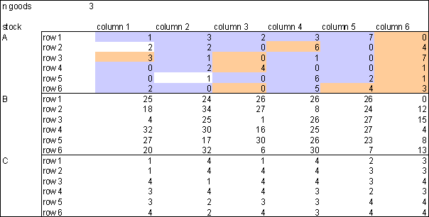
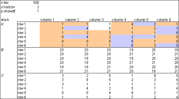
The main design guideline was to use user-defined-functions. By this the full functionality of a spread-sheet program can be used, as changes in variables are immediately reflected in results (as far as computing time allows for immediacy). This approach allows the construction of initial distributions of wealth and interactive observation of the behaviour of the model. The following figures give an overview of how the model works. The VBA Code can be found in Appendix A.

3.3

Only one parameter - the number of goods - has to be specified (in this case 3). The initial distribution then needs to be put into a matrix (a range in terms of Excel). The only requirement is that the number of rows must be a multiple of the number of goods specified initially.

3.4

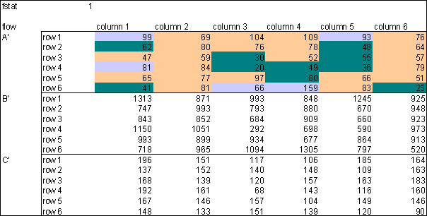
The colours result from a classification by fuzzy clustering into 2 clusters (rich/poor). The clustering is achieved by the fuzzy-c-means clustering algorithm. The fields with blue background colour indicate that their membership in cluster with rank 1 is above 60%. The fields with a red background have a cluster membership in cluster with rank 2 above 60%. Uncoloured fields do not fulfil either of the two conditions. The clusters get ranked according to Euclidean norm of their cluster centres. The parameters for cluster weight can be chosen (in this setting 1.5 was used).

Figure 1. Initial wealth with 3 Goods in a 6 × 6 world, Spreadsheet

3.5

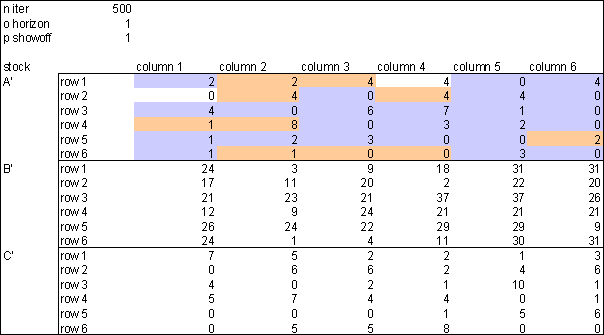
The example shows an initial distribution where goods A and C are owned fairly low in number. Good B is owned in larger quantities. In contrast to good A and good B, good C is distributed fairly equal. This initial distribution was generated by using random numbers from beta distributions, each good with a different parameter setting and truncating the random numbers to integer values. After 500 trade runs with an observation horizon 1 (agents can observe other agents that are no more than 1 row or column apart) and a show off probability of 100% the following result is calculated:

Figure 2. Stock after 500 trade runs, observation horizon 1, show off probability 100%

Note that the evenness of distribution of wealth of good C has been lost.

3.6

The flows show the following structure:

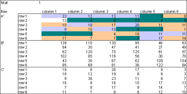
Figure 3. Flow in 500 trade runs, observation horizon 1, show off probability 100%

The figure is obtained by adding the absolute value of goods flows throughout the trade runs. The colours now refer to 3 clusters. Blue is again the cluster which ranks highest in Euclidean norm of the cluster centre, green ranks lowest. So blue agents trade most, green ones trade lowest. Not surprisingly, the given case clusters show a cohesive pattern, as deals are only made with direct neighbours.

3.7

Let us compare the result with an increased observation horizon:

Figure 4. Stock after 500 (137) trade runs, observation horizon 2, show off probability 100%

As an immediate consequence the system reaches equilibrium (a fixed point) after 137 trade runs. Equilibrium is defined as a situation in which no more deals occur or when a cycle is reached.

3.8

From the results presented one can see, that equilibrium is primarily characterised by an even distribution in good B. Other goods are not distributed as evenly as good B. This is due to fact that individual showoffs only occur with the good that an agent owns most in number.

3.9

This leads to the question how many iterations are needed to reach equilibrium with observation horizon 1. The result is 159,219 trade runs, which is a big difference. The clustering of the flows does no longer show the same pattern:

Figure 5. Flow in 500 (137) trade runs, observation horizon 2, show off probability 100%

It is worth mentioning that a further increase of the observation horizon to 3 does not give a different result to observation horizon 2. In a 6 × 6 world observing other agents that are no more than 2 rows or columns apart (in each direction) is a situation that nearly amounts to "every agent observes every other agent".

3.10

I would like to add the following comments regarding usage and limits of the model

• Given the rules of the model, an agent that owns no more than 0 (or 1) of every tradeable good will never participate in any deal. This allows for modelling of sparse populations.
• Neither exclusion nor inclusion can happen as a result of the dynamics of the system. Agents can become wealthier or poorer but they never drop out of business.

Characteristics of Solution Paths

3.11

In order to observe solution paths the following statistics are collected:

• Distance to mean: As the total number of every good stays the same during all iterations it is straight forward to add up the absolute values of the differences of ownership of every agent with the mean. To make this measure comparable to the mean used above, this sum is also divided by the number of agents. Approaching the fixed point observed before this statistics must decrease in value. To be more exact equilibrium is better described as a set of fixed points, where distribution of wealth is almost even and no further proposals are made.
• Activities: The number of proposals following show off, the number of proposals following price differences and the number of deals are recorded and shown.
• Weighted average prices: In terms of prices (understood as exchange rates) the weighted average prices are calculated for every trade run and recorded. If no deals occur the weighted average prices is set to zero.

Although these statistics amount to an outside observation of the larger environment it is nevertheless interesting for studying the behaviour of the system. The following sections show the statistics for the examples shown above.

Distance to Mean

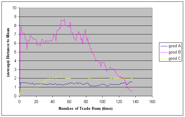
3.12

The development of the average distance to mean is shown in the following figures

Figure 6. Distance to mean (even distribution), observation horizon 1; only the first 500 trade runs are shown

3.13

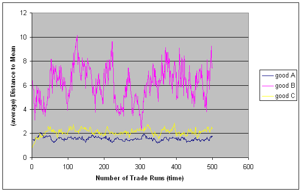
The next figure will show the development of the distance to mean given the same initial distribution but an observation horizon 2. As indicated above, the system reaches equilibrium after 137 trade runs. In both cases the distance to mean regarding good C is increased during the first trade runs, where as the distance to mean of good B lowers. At a certain point this development stops and the system shows a fairly irregular pattern. There are instances when the distance to mean is even bigger than the initial distribution for all goods. This irregular pattern finally breaks down and the distance to mean of good B (the good that is most abundant) falls below 1, the system reaches equilibrium.

Figure 7. Distance to even distribution, observation horizon 2

The difference between observation horizon 1 and 2 is, that the irregular phase lasts about 150.000 trade runs given observation horizon 1, and merely 80 trade runs given observation horizon 2.

Activitites

3.14

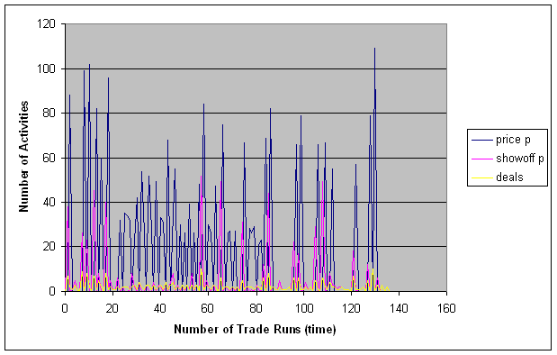
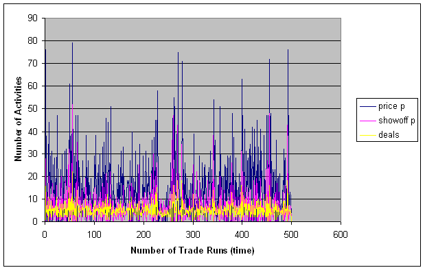
The next statistics collected are the number of activities. As expected the increased observation horizon leads to more proposals but a smaller number of accepted deals, because only one best deal among all proposals (per pair of exchangable goods) is chosen.

Figure 8. Activities statistics, observation horizon 1; first 500 trade runs

Figure 9. Activities statistics, observation horizon 2

Prices

3.15

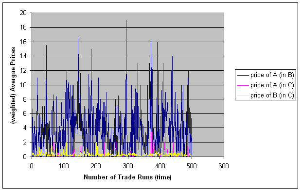
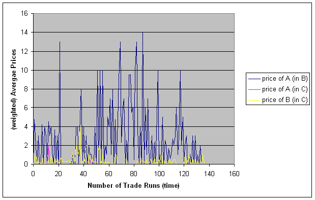
The last statistics collected are (weigthed) average prices:

Figure 10. Price statistics, observation horizon 1; first 500 trade runs

Figure 11. Price statistics, observation horizon 2

The qualitative behaviour appears to be the same in observation horizon 1 and 2.

Characteristics of Classes of Solutions

3.16

Scenarios were defined and evaluated by Monte Carlo simulation, in order to analyse the system for whole classes of initial distributions. All of the scenarios (except scenario 1a) refer to a 6 × 6 world, 3 goods, an observation horizon 1 and a show off probability 1 (deterministic). Scenario 1a analyses the impact of different show off probabilities. As these sizes can be given as parameters to the software developed examples have been calculated also in a 4 × 4 and 12 × 12 world. A world with 12 × 12 agents is closer to the size of an early homo sapiens group, as explained in Dunbar (1996, p. 63).

3.17

In the 4 × 4 world an observation horizon 1 is nearly equivalent to the situation of every agent observing every other agent. So this world was considered too small. In a 12 × 12 world the limits of a default personal computer regarding an acceptable performance for model exploration were reached.

3.18

The 6 × 6 world shows rich behaviour such as cycles of different length, quick and late convergence.

3.19

The following scenarios have been defined

• Scenario 1: All three goods are distributed according to a uniform distribution in the interval [0,7] truncated to integer values. See Mood et al. (1974, p. 540) for the probability density function of a uniform (or rectangular) distribution.
• Scenario 1a: The showoff probability is varied.
• Scenario 2: All three goods are (still) distributed according to a uniform distribution - but the intervals vary. This is to reflect that goods vary in their abundance (scarcity). The intervals used are [0,7], [0,11], [0,5].
• Scenario 3: The intervals stay the same, but the distributions are changed. The distribution of the first good stays unchanged. For the second and third good Beta distributions are used to compute the initial distribution of wealth. For good B the following parameters are used: a = 2, b = 1. For good C the values of the parameters are reversed. See again Mood et al. (1974, p. 540) for the probability density function of a ([0,1] standardised) Beta distribution.
• Scenario 4: intervals and distributions are the same as scenario 3. The parameters are varied to a = 3, b = 1 for good B, good C holds again the parameters of good B in reverse order.

Scenario 1

3.20

Each scenario is based on the selection of 100 initial distributions of wealth (goods A, B, C) according to the rules given above. For each of the initial distributions a maximum of 2000 trade runs is computed. The following table gives information that was aggregated from the 100 cases of this scenario. Details can be found in Appendix B.

3.21

In order to check for the robustness of the scenarios, the scenarios were repeated (with further 100 cases) and their results compared. There were no differences in qualitative terms (types of cycles, number of trade runs). In quantitative terms the differences of the aggregated results were considered small enough.

Table 1: Aggregated results scenario 1
	last run no deals	number no deals	episode length	total A+B+C
mean	37	7	7	326
median	35	6	6	325
std deviation	12	4	5	22
std deviation in %	32%	56%	73%	7%

3.22

The table contains the following columns:

• Last run non deals: This refers to the number of the trade run, when no more deals are made in 2 consecutive steps and equilibrium is reached. The system dynamics (type 2^nd order difference equation) demands that two steps need to be checked. In this case of a fairly even distribution of all goods the median number of trade runs needed to reach equilibrium is 34.5. The comparatively low standard deviation (in % of the mean) indicates that the behaviour is fairly homogenous.
• Number no deals: The rules of the model imply situations where no deal gets accepted. This is primarily due to repeated proposals following the arbitrage rule being not accepted given the no short selling condition. At these temporary rest points the system settles down - for one moment - and the activity rule (proposals following show off) generates further business for the next rounds. The number of these temporary rest points is given. They mark the beginning and end of so called episodes.
• Episode length: The (average) length of episodes is given by the number of trade runs (i.e. the last trade run no deals) divided by the number of temporary rest points (number no deals).
• Total A+B+C: The total wealth was recorded because the possible number of states of the system (restricted to temporary restpoints) is given by (6 * 6)^a+b+c-1, where a, b, c denote the total number of goods A,B,C in the system. The -1 in the exponent is due to symmetry caused by the torus. The total serves as a control variable, because a longer journey to equilibrium could also be due to the fact, that there are more states.

3.23

Although the quantitative results are not very surprising, this scenario shows rich qualitative behaviour that does not emerge in the other scenarios:

• Cycles: Nearly half of the cases obtained end with a cycle. The detected cycle lengths are 1, 2 and 5. As these lengths are calculated as distances between the last saved state that equals the actual state (considering symmetry), they refer to period lengths of 2, 3, and 6. A period of length 1 indicates a fixed point.
• Cycle within episodes: As the exploration part of the software checks for cycles only at the temporary rest points (because they can be tested more easily) cycles that appear within an episode are not detected automatically. However 3 of these cases appeared.

All of the observed cycles do appear in states that are very close to the equilibrium.

3.24

If the mapping would be continuous, the observed period length 3 would point to chaotic behaviour by Sarkovskii's theorem^[28]. As the system only has a finite number of states it cannot be chaotic in terms of the definition. See Lawvere (2002, p.317) for the definition of a chaotic observable on a dynamic system.

Scenario 1a

3.25

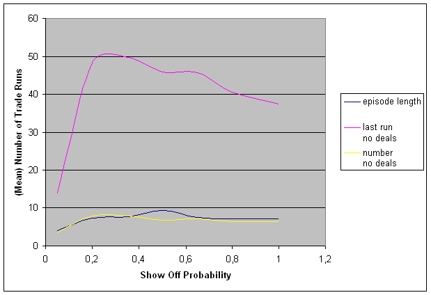
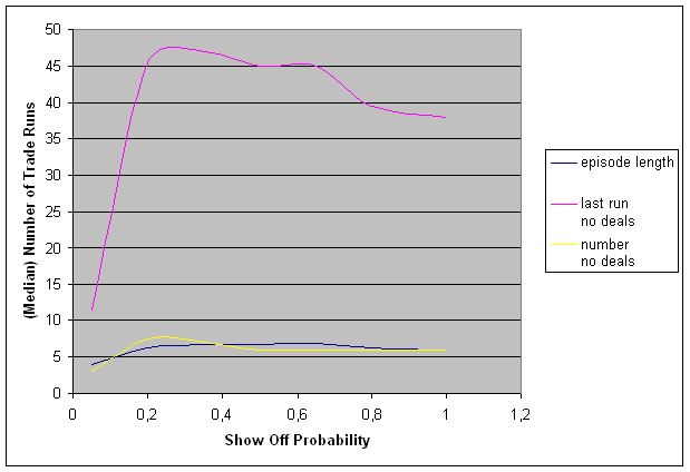
Scenario 1a shows the influence of the show off probability on the characteristics of solutions to the model. The results are given in the following figures:

Figure 12. Means of characteristics varying with showoff probability

Figure 13. Median of characteristics varying with showoff probability

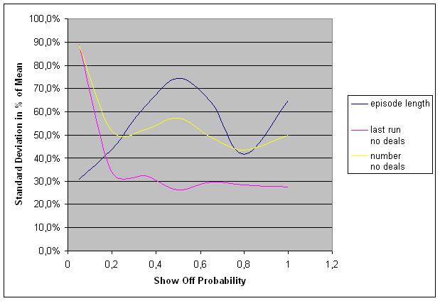
Figure 14. Relative Standard deviation of characteristics varying with showoff probability

3.26

The simulations indicate that episode length and the number of temporary rest points are fairly invariant to changes of the show off probability when the mean or median of the cases is considered. This is reasonable as episodes largely depend on the continuation of deals by applying the arbitrage rule. However the relative deviation shows an interesting pattern.

3.27

Regarding the number of trade runs required to reach equilibrium (last run no deals), a peak is achieved at a show off probability of 20% that is slowly decreasing to the value when show off is deterministic.

Scenario 2

3.28

Scenario 2 is very similar to scenario one, except that the intervals in which the goods A, B, C are distributed are no longer the same. Good B is must abundant. Good C is scarcest.

Table 2: Aggregated results scenario 2
	last run no deals	number no deals	episode length	total A+B+C
mean	75	8	10	361
median	55	7	8	364
std deviation	82	5	5	25
std deviation in %	109%	62%	55%	7%

Compared to scenario 1 the mean number of trade runs required to reach equilibrium (last run no deals) more than doubles, the median moves from 34.5 to 54.5. The relative standard deviation at least doubles. The number and the length of episodes are increased only slightly (in all measures).

3.29

Cycling occurs far less, i.e. in about 14% compared to nearly half of the cases in scenario 1. A cycle of period length 4 is observed.

Scenario 3

3.30

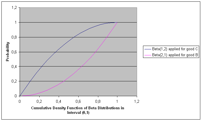
In Scenario 3 the unevenness of distribution is further increased. The initial wealth regarding good B (still most abundant) is now retrieved from a beta distribution with parameter values: a = 2, b = 1. The cumulative distribution function can be seen in the figure below. This parameter setting moves the mass of the distribution slightly to the right, i.e. more agents own a higher amount of good B. For the scarcest good C, the situation is intensified by selecting parameter values: a = 1, b = 2 and moving the mass of the distribution slightly to the left. The cumulative distribution function is shown below:

Figure 15. Cumulative Β(1,2) and Β(2,1) distribution functions

3.31

The results are summarised in the following table:

Table 3: Aggregated results scenario 3
	last run no deals	number no deals	episode length	total A+B+C
mean	151	11	12	397
median	97	9	11	397
std deviation	190	9	7	22
std deviation in %	126%	76%	54%	6%

It is interesting that the step from scenario 1 to 2 shows a similar pattern as the step from scenario 2 to scenario 3. Mean and Median of the required number of trade runs to reach equilibrium nearly double again. The number of deals and episode length increase only slightly. Cycling (with period length 2) occurs only once.

Scenario 4

3.32

The final scenario 4 is characterised by further intensifying abundance of good B and scarcity of good C. The unevenness of the total distribution of wealth is also increased.

3.33

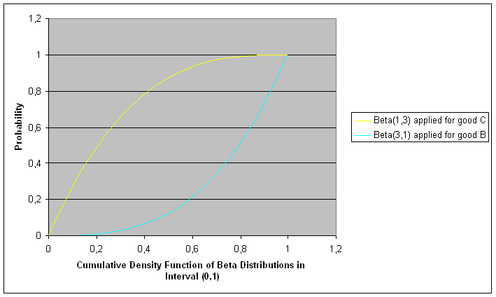
The next two figures show the cumulative distribution functions from which the initial endowments regarding good B and good C were calculated.

Figure 16. Cumulative Β(1,3) and Β(3,1) distribution functions

The following results were obtained:

Table 4: Aggregated results scenario 4
	last run no deals	number no deals	episode length	total A+B+C
mean	291	16	15	414
median	180	13	14	414
std deviation	332	12	9	17
std deviation in %	114%	78%	62%	4%

The pattern that was observed by moving from one scenario to the next is affirmed. Mean and median of the required trade runs to reach equilibrium nearly double again. The number of episodes and their length increases only slightly. No more cycles are observed.

Conclusion

4.1

At the onset of this work there has been the idea to model what was called a simple Luhmann economy by an agent-based model. Studying the behaviour of the model showed conformity to Niklas Luhmann's hypothesis, that the economy starts from and produces further inequality in order to continue (see Luhmann 1988, p. 112).

4.2

The study of the behaviour of the system has shown:

• The number of trade runs needed by the system to reach an end of its autopoiesis (either a fixed point or a closed cycle, also understood as equilibrium) is significantly enhanced by the extent of unevenness of initial wealth.
• A comparatively long path to the end of autopoiesis (equilibrium) can be observed, when the following conditions are met:
  • uneven initial distribution of wealth (i.e. sufficient "disorder" in the environment)
  • sufficient large numbers of some, but not all goods (abundance/scarcity)
  • an observation horizon that does not imply every agent sees every other agent
  • a showoff probability above 20% (i.e. sufficient "disorder" in the environment)
• Given these conditions the system maintains a level of unevenness (subpaths seem to move away from equilibrium) and shows fairly irregular patterns for a considerable amount of trade runs (time) before it suddenly breaks down and reaches equilibrium. This timeframe may be long enough (our example with only 36 agents, 3 goods altogether 900 in number needed more than 150.000 trade runs) to justify Niklas Luhmann's observation that the economy produces unevenness from unevenness.
• Although individual economic communication drives towards equilibrium, equilibrium of the system is upset for long periods of time due to historical conditions and other economic communications. The model does not show a smooth path towards equilibrium.
• The observation indicates that the length of episodes is less sensitive to the parameters that guide unevenness
• Although cycles (with various period lengths) have occurred in the simulations only "close" (in terms of average distance to mean) to equilibrium ones were observed. There are no indications that similar cycles (with presumably longer period lengths) could also occur at levels farther away from equilibrium.
• The emergence of systems within systems was not studied in this simple model. However the model describes how activities are caused by prior observations of activities. The model maintains a certain distance from equilibrium by its own operations - not forever but for a considerable amount of time.

4.3

The model turned out to be too simple to show distinctive patterns of differentiaton although fuzzy clustering has proved to be an aid in the interactive search for types of sytem behaviour. The development and specification of the model has given rise to further questions, such as:

• What are the necessary modelling assumptions to allow for credit, agents moving between locations and more complicated decision rules?
• What are the effects of combining the economic and other function systems (e.g. law, politics), when these systems operate with the same agents and serve each other as "irritating" environments?
• How do different and more complicated communication patterns between agents (e.g. networks) affect the simulations?

It also points to directions for future enhancements and so gives ideas how these questions might be answered.

Notes

¹see Luhmann (1995), p. 103-136

²see Luhmann (1995), p. 446-447: Self-referential, autopoietic reproduction would not be possible without an anticipatory recursivity.

³Luhmann (1989) includes a glossary of the most frequent terms in English.

⁴see Luhmann (1989) for a concise description of societal function systems. The differentiation of (world) society into function systems (and its primacy) is among the core theorems of Niklas Luhmann's theory. Note that both society as a whole and its function systems are defined as social systems.

⁵see Luhmann (1995), p. 412: Society is a system for which an encompassing system does not exist

⁶see Luhmann (1988), p. 413: society is the result of evolution. One does also speak of “ermergence”. ... there is today no other theory (except evolution) that can explain the emergence and reproduction of structures of the social system society

⁷see Luhmann (1988), p. 232: One can oppose the theorem of a certain structural isomorphism of meaning and money - if one means something different by meaning. But insights, that are worth to be preserved are possibly lost in this case.

⁸see further Luhmann (1993), pp 175-186

⁹see Axelrod (1997) p. 3: Agent-based modelling is a third way of doing science. Like deduction, it starts with a set of explicit assumptions. But unlike deduction, it does not prove theorems. Instead, an agents-based model generates simulated data that can be analysed inductively

¹⁰see Luhmann (1995), p. 43: An element is, what for a system functions as a not further dissoluble unity;

¹¹see further Luhmann (1995), p. 240: To the Question, what are the parts of social systems, we give a double answer: Communications and their attribution as action.

¹²see further Luhmann (1995), p. 78: The system builds itself from instable elements, that last only a short amount of time - or as in the case of action have no duration by themselves. ... A stable system consists of unstable elements. The stability is a consequence of itself being a system, not of the elements. Still the system is constituted by its elements - in this case events. It has no basis for duration outside of these events (this is why we experience the present necessarily as short)

¹³see Luhmann (1995), p. 398: The theory of events and structures plus the theory of expectations are put together by the proposition that structures of social systems are made of expectations, that they are structures of expectations, and that for social systems - because they temporalise their elements as events of action - there are no other options to build structures. That means: structures do only exist as present structures

¹⁴see further Luhmann (1995), p. 363: Expectations are a primitve technique. This technique can be used nearly without prerequisites. It is not necessary to know who you are or what you know about your environment. One can have an expectation, without knowing the world - for pure luck. It is solely important, that the expectation can be used by the autopoiesis, so that the access to connecting reality constructions (“Vorstellungen”) is sufficiently pre-structured.

¹⁵See further Luhmann (1995), p. 149: In a somewhat different formulation, one can say: communication transforms the difference between information and utterance into the difference between acceptance or rejection of the utterance.

¹⁶see Luhmann (1995), p. 203: If communication is defined as synthesis of three selections (the unity of information, utterance and understanding), it is realised when and to what extent understanding happens. Everything further happens outside the unity of an elementary communication. This is not to be confused with the acceptance of refusal of the (communicated, i.e. understood) selection as a basis for own behaviour. But it cannot be ignored.

¹⁷For the definition of information (what was said?), utterance (was it said?) and understanding (selection of meaning) see Luhmann (1995), pp.137-175

¹⁸See Luhmann (1988), p. 26: that means, the structures of a system can only be varied by the systme's own operations. These operations themselves depend on the structures of the system.

¹⁹see Luhmann (1995), p. 92: Psychic and social systems evolved by means of Co-evolution

²⁰Psychic systems are like social systems defined as autonomous systems processing meaning. Their elements are thoughts, not communications, see Luhmann (1995), p. 59

²¹The term n-to-m refers to n agents performing the task of Alter, m agents performing the task of Ego. Note that in Luhmann's terminology Ego is the agent that understands information and utterance of the agent Alter. Alter is the agent that has provided an offer for communication (an action), as attributed (understood) by Ego.

²²The choice of the lexicographic smallest index (instead of random) was preferred at this stage of model development to be able to reproduce results.

²³The motivation to show-off lies outside the economic system. It is not governed by bounded rationality focussed on ownership of goods. Probability is used to separate autonomous system dynamics and environmental dynamics. The same holds for the initial distribution of wealth, which is also outside the dynamics of the economic system.

²⁴see xxii

²⁵see xxii

²⁶see xxii

²⁷The term larger environment refers to the environment of agents as observable to the constructer of the model, who has - compared to the agents within this model - superior observation capacity

²⁸see Devaney (2003), p. 60: Let f:R into R be continous. Suppose f has a periodic point of period 3. Then f has periodic points of all other points.

References

AXELROD, Robert M. (1984), The Evolution of Cooperation. Harper

AXELROD, Robert M. (1997), The Complexity of Cooperation. Princeton

DEVANEY, Robert L. (2003), An Introduction to Chaotic Dynamical Systems, 2nd Edition. Westview Press

DUNBAR, Robin I. M. (1996), Grooming, Gossip and the Evolution of Language. Harvard University Press, 1998

JOAS, Hans and KNÖBL Wolfgang (2004), Sozialtheorie, Zwanzig einführende Vorlesungen. Suhrkamp, 2004.

KRON, Thomas and DITTRICH, Peter (2002), "Kontingenz nach Luhmann - ein Simulationsexperiment" in Kron, Thomas (Ed.) (2002), Luhmann modelliert. Leske+Budrich

LAWVERE, F. William and Schanuel, Stephen H. (1997), Conceptual Mathematics. Cambridge University Press, 2002

LEYDESDORFF, Loet (2004), "Meaning, Anticipation and Codification in Functionally Differentiated Systems of Communications" in Kron, Thomas, Schimank, Uwe, Winter, Lars (eds), Luhmann simulated - Computer Simulations of the Theory of Social Systems. Hamburg, LIT-Verlag (in Vorbereitung) 2005.

LUHMANN, Niklas (1973), Zweckbegriff und Systemrationalität, 6. Auflage. Suhrkamp, 1999

LUHMANN, Niklas (1975), Macht. Lucius & Lucius. Suhrkamp, 2003

LUHMANN, Niklas (1984), Soziale Systeme, Grundriß einer allgemeinen Theorie. Suhrkamp, 1999

LUHMANN, Niklas (1988), Die Wirtschaft der Gesellschaft. Suhrkamp, 1999

LUHMANN, Niklas (1989), Ecological Communication (translated by John Bednarz, Jr.). The University of Chicago Press

LUHMANN, Niklas (1993), Risk: A Sociological Theory (translated by Rhodes Barrett). Aldine De Gruyter

LUHMANN, Niklas (1995), Social Systems (translated by John Bednarz, Jr.). Stanford University Press

LUHMANN, Niklas (1997), Die Gesellschaft der Gesellschaft. Suhrkamp, 1999

MEHLMANN, Alexander (1997), Wer gewinnt das Spiel. Vieweg

MILGROM, Paul (2003), Putting Auction Theory to Work. Cambridge University Press

MOOD, Alexander M. and Graybill, Franklin A. and Boes, Duane C. (1974), Introduction to the Theory of Statistics. McGraw Hill, 1983

NELSON, Richard R. and WINTER, Sidney G. (1982), An Evolutionary Theory of Economic Change. The Belknap Press of Harvard University Press

PINGLE, Mark and TESFATSION Leigh, 2003, "Evolution of Worker-Employer Networks and Behaviors Under Alternative Non-Employment Benefits: An Agent-Based Computational Study", pp. 253-284 in Anna Nagurney (ed.), Innovations in Financial and Economic Networks. Edward Elgar Publishers, 2003.

SIMON Herbert A. (1951), "A Behavioural Model of Rational Choice", Quarterly Journal of Economics 69, pp. 99-118. Reprinted in Models of Man. Wiley, New York, 1957

WOLKENHAUER, Olaf (2001), Data Engineering. Wiley

Return to Contents of this issue

© Copyright Journal of Artificial Societies and Social Simulation, [2005]