©Copyright JASSS

JASSS logo ----

Piergiuseppe Morone and Richard Taylor (2004)

Small World Dynamics and The Process of Knowledge Diffusion: The Case of The Metropolitan Area of Greater Santiago De Chile

Journal of Artificial Societies and Social Simulation vol. 7, no. 2
<https://www.jasss.org/7/2/5.html>

To cite articles published in the Journal of Artificial Societies and Social Simulation, reference the above information and include paragraph numbers if necessary

Received: 07-Feb-2004    Accepted: 12-Feb-2004    Published: 31-Mar-2004


* Abstract

This paper aims to understand some of the mechanisms which dominate the phenomenon of knowledge diffusion in the process that is called 'interactive learning'. We examine how knowledge spreads in a network in which agents have 'face-to-face' learning interactions. We define a social network structured as a graph consisting of agents (vertices) and connections (edges) and situated on a grid which resembles the geographical characteristics of the metropolitan area of Greater Santiago de Chile. The target of this simulation is to test whether knowledge diffuses homogeneously or whether it follows some biased path generating geographical divergence between a core area and a periphery. We also investigate the efficiency of our 'preference' model of agent decision-making and show that this system evolves towards a small-world type network.

Keywords:
Agent-based, Chile, Inequality, Knowledge, Network, Small world

* Introduction

That the advance of knowledge lies at the core of modern growth process is more than an inference from the growth accounts. It is a perception enforced by well over a century of common experience. Economists have therefore applied themselves to learning more about the ways that practical knowledge is gained and exploited. A new outlook has developed and spread. It is not yet well defined (Abramovitz 1989)
1.1
The dynamic nature of the knowledge-based economy has increasingly directed the attention of researchers towards process-orientated perspectives and interdisciplinary approaches. Evolutionary economics has emerged as a leading example of this trend. By encouraging the development of new theory-building tools based on evolutionary principles, as well as improving our ability to describe learning and adaptation processes found in empirical research, it undeniably has shaped our understandings of the information society. Agent-based modelling is one such tool that allows us to reflect on existing theory, and to apply our evolutionary models to relevant case studies.

1.2
Adopting the agent-based approach, this paper presents our research investigating knowledge flows in a network of interacting individuals. We focus upon the processes of diffusion and learning, and the emerging network characteristics that result from these interactions. We explore these dynamics by means of a calibrated simulation model, using socio-geographical data from the Greater Santiago de Chile case study.

1.3
To our understanding, the processes of learning and knowledge diffusion are still largely undiscovered and require substantial theoretical and empirical efforts in order to be properly understood. The nexus linking education and personal income is well established in the labour economic literature. It has been thoroughly investigated both theoretically and empirically and its main conclusion is that investments in human capital have a positive impact on one's future income. The learning process through which labour force builds up human capital has then been divided into schooling and on-the-job experience.

1.4
In this work, following Morone (2001), we argue that the process of human capital creation should be decomposed into two distinct learning processes: individual learning and interactive learning. The first is basically the learning process which takes place at school or through training courses, while the second, neglected by the literature until now, is the learning process which takes place through simply every-day interactions which each person has with her/his acquaintances.

1.5
The focus of this work is precisely this second learning process. We will study how interactive learning affects the knowledge creation in a middle-income country like Chile. We decided to focus on the Chilean case because of its particularly biased wage distribution and its exponential returns to schooling.[1]

1.6
The main target of this work is to model one possible type of interactive learning known as 'face-to-face' learning. Departing from previous studies on knowledge diffusion, we aim to develop a model which takes into consideration the complexity of the process of knowledge acquisition. In doing so we define a cognitive structure for each agent (cognitive map) and use this structure to define the process of knowledge acquisition.

1.7
The paper is structured as follows: section 2 revises briefly the existing literature on informal knowledge diffusion. In section 3 we present a formal model which investigates how knowledge spreads among agents situated on a grid composed of several neighbourhoods. Section 4 develops the concept of Cognitive Map (CM) and elaborates on the processes of knowledge diffusion and accumulation in the presence of a complex cognitive structure. Section 5 then introduces the case study and shows the results of the simulation exercise. Finally, section 6 concludes the paper.

* Reviewing Literature On Interactive Learning

2.1
The learning process which takes place simply by interacting within a neighbourhood can be considered as a social externality. For instance, the diffusion of a new technology is a positive externality, which is generated by the informal interaction of entrepreneurs. Nonetheless, learning from neighbours can also represent a negative externality. Consider, for instance, the problem of children in a poor neighbourhood choosing whether to pursue higher education or drop out of school. If in such an environment the most popular decision were dropping out, this would represent a negative externality for those children facing the choice, subject to social influence.

2.2
Most studies found that social learning plays a positive role in determining the long-term equilibrium. Ellison and Fudenberg (1993) developed a model in which agents consider the experience of neighbours in deciding which of two technologies to use. Their work is structured around two simple models of the learning environment. First, they consider a homogeneous population which reacts identically to the two technologies, with one technology being superior to the other; subsequently they introduced heterogeneous agents who consider the two technologies in different ways. In the first case the issue is whether the better technology will be adopted, while in the second case, the question is whether the two technologies will be adopted by the appropriate players. In both environments agents use exogenously specified 'rules of thumb' that ignore historical data but might incorporate a tendency to use the more popular technology. Under this condition, the outcome of this study suggests that "even very naïve learning rules can lead to quite efficient long-run social states", but adjustment can be slow when a superior technology is first introduced (Ellison and Fudenberg 1993: 637).

2.3
In a subsequent paper (Ellison and Fudenberg 1995), the authors focused their attention on patterns of information exchanges, studying the way in which word-of-mouth communication contributes to aggregate information of individual agents. They defined a nonstrategic environment composed of homogeneous agents who face the decision of choosing one of two products. Their findings show how "despite the naïve play of individuals, this type of information flow may lead to efficient learning on the social level, and that social learning is often most efficient when communication between agents is fairly limited" (Ellison and Fudenberg, 1995: 120).

2.4
Bala and Goyal (1995) analysed social learning in an organisational environment in which agents have a time-limited life experience and heterogeneous beliefs. Departing from the original work of Kiefer (1989), they consider the case of a monopolistic firm attempting to calculate its true demand curve. "The learning process - adopted by the authors - is then one in which the sequence of managers learn about the demand curve through their own actions as well as the experience of earlier managers" (Bala and Goyal 1995: 303). In this case, again, learning from others augments the probability of converging to the set of ex-post optimal actions.

2.5
Subsequently, Bala and Goyal (1998) investigated the relation between the structure of social networks and learning processes in a world where agents learn from currently available social information, as well as from past experiences (as opposed to the previous works of Ellison and Fudenberg). Their findings show that the structure of the neighbourhood has important implications for the likelihood of adopting new technologies, for the coexistence of different practices, and for the temporal and spatial patters of diffusion in a society. More precisely, they showed how neighbourhood structures characterised by the presence of locally independent agents (i.e. agents with non-overlapping neighbourhoods) generally facilitate social learning.

2.6
A common way of modelling the mechanisms of social learning and technology diffusion makes use of evolutionary game theory. Several authors examined local interaction games[2] in which each agent's payoff depends on the actions of his/her neighbours. Most of these studies pointed out that local interaction might result in the diffusion of personal behaviours in certain dynamic systems. In a recent work, Morris (2000) extended this finding, linking the occurrence of social learning (that he calls contagion) to some qualitative properties of the interaction system such as cohesion, neighbour growth, and uniformity. Chwe (2000) modelled social learning as dependent on both social structure and individual incentives. In this way he obtained a model that he called a 'local information game' as, he argued, "locality is represented by information and not necessarily by payoffs […]. Local interaction games make sense for local coordination, such as keeping our street clean; for 'big' coordinations such as political changes, informational locality is more appropriate" (Chwe 2000: 11).

2.7
Along with the speed of new technologies' diffusion, several researchers have focused on the impact of peers' behaviour upon individual decisions in several areas such as propensity to crime, use of drugs, school dropout and school attainments. For instance, the role model provided by good students might generate positive spillovers in the sense that peer students may imitate successful behaviours. Nonetheless, "when social interactions act as strategic complementarities between agents, multiple equilibria may occur in absence of any coordination mechanisms" (Brock and Durlauf 1995: 1). The school-based interaction was studied by Bénabou (1993) in his model of occupational and residential choices. The author shows that when the cost of individual education is a decreasing function of investment decision of one's neighbours, neighbourhoods can exhibit multiple equilibria in the steady-state level of human capital.

2.8
Durlauf (1996) showed how these spillovers can have significant distributional effects generating stubborn inequality in the long run. Income inequality "emerges through the interaction of positive feedback structure between members of a common neighbourhood with the tendency of families to stratify themselves endogenously into economically homogeneous neighbourhoods" (Durlauf 1996: 505).

2.9
The notion of 'positive feedbacks' means, in the words of Durlauf, "that the income distribution of neighbourhoods will strongly affect the future economic status of children within the community" (Durlauf, 1996: 505). A similar argument was raised by Glaeser, Sacerdote and Scheinkman (1996), who argued that social interactions can explain large differences in community crime rates.

2.10
What all the studies considered so far have in common is the fact that learning from neighbours occurs and that under certain conditions it leads to (highly unequal) multiple equilibria. Yet, none of these studies goes beyond a binary definition of learning. If there is a new technology, agents can either learn of its existence, and hence adopt it, or stay in their initial state of ignorance. Pupils that live in 'good' neighbourhoods have good chances of imitating good role models, while pupils who live in 'bad' neighbourhoods are more likely to imitate bad role models and hence end-up in perpetuating the initial differences. In other words, learning is defined and modelled as an imitational process deprived of its real complexity. In the economic literature there are few attempts to model informal knowledge diffusion in a more complex way. We will now examine these works.

2.11
Jovanovic and Rob (1989) presented a model in which knowledge was defined as a public good which is exchanged through pairwise meetings. The authors define incremental improvements in knowledge as a complex process of assembling different ideas by means of information exchange by heterogeneous agents. The new insight brought by Jovanovic and Rob is that knowledge is defined as something more complex than a binary variable and, therefore, that growth of knowledge can be defined as an interactive process tightly linked to its diffusion.

2.12
Cowan and Jonard (1999) made a subsequent attempt to study the effects of incremental innovations and their diffusion over a network of heterogeneous agents. In their model, knowledge is considered as a vector of values and is exchanged via a simple process of barter exchange. Depending on the network structure, the authors found that there is a trade-off between the speed of knowledge diffusion and the variance of knowledge. In other words, there is a spectrum of states of the world varying from a situation of high knowledge inequality and fast knowledge diffusion (i.e. small-world) to the opposed situation, more equal in terms of knowledge variance but less efficient in terms of knowledge diffusion.

2.13
Along the lines of Cowan and Jonard (1999), Morone and Taylor (2004) defined a model in which agents exchange knowledge by means of face-to-face interactions. The network structure was endogenous to the model and could vary over time. The authors showed how small-world networks emerged and coexisted with both a very unequal and a very equal diffusion of knowledge, depending upon the initial conditions. The model presented in the following section could be considered an extension of Morone and Taylor (2004) as it departs from similar assumptions but develops a more complex learning structure.

* Model Description

3.1
We assume a population of N agents distributed over a grid that resembles the geographical configuration of the metropolitan area of Greater Santiago de Chile. The grid is divided into 34 portions, each corresponding to a defined district of Santiago and thus having different dimensions and different population densities. Each agent is initially assigned a district and then allocated to a cell at random within that district. However, agents do not occupy all the cells of the grid, and each occupied cell can have only one agent. Neighbourhoods, which may contain cells from several districts, are constructed according to the von Neumann definition: those cells adjacent in the four cardinal directions and within the agent's visible range. The initial local-network is created by connecting an agent with all other agents located within her/his neighbourhood. We also define a cyber-network as the ideal network connecting all those agents who have access to the Internet. The cyber-network generates a second system which has no geographical dimension but connects agents located in far distant regions through ICT support. As opposed to the local-network, all agents who have access to the Internet are neighbours within the cyber-network (i.e. the visibility is equal to the size of the system). Each agent has a list of acquaintances which includes the members of the local-network and the cyber-network. The data which are used to initialise the model are a sub-sample of the 1998 edition of the Encuesta de Ocupación y Desocupación, and will be described more fully later.

3.2
Our geographical network is expressed in graph notation following the standard definition: "a graph G consists of a nonempty set of elements, called vertices, and a list of unordered pairs of these elements called edges" (Wilson and Watkins 1990). In our simulation, vertices correspond to agents and edges are the agents' connections. Formally, we have G (I, Γ), where I = {1,…, N} is the set of agents, and Γ = {Γ(i), iI} gives the list of agents to which each agent is connected. This can also be written Γ(x) = {(yI \ {x} | d(x, y) -# ν) (yω)}, where d(x, y) is the length of the shortest path from agent x to agent y (i.e. the path which requires the shortest number of intermediate links to connect agent x to agent y), ν (visibility), as already mentioned, is the number of cells in each direction which are considered to be within the agent's spectrum, and ω defines the cyber-space, which by definition encompasses all those agents endowed with ICT facilities (i.e. computers connected to the Internet). Intuitively, Γx (we will use this notation rather than Γ(x) from now on) defines the neighbourhood of the agent (vertex) x.

3.3
The unit of time we define in our model is called the cycle. In each cycle, all individuals are sorted into a random order, and each is then permitted to interact with one acquaintance. Each interaction is aimed at diffusing knowledge. Each agent is endowed with a cognitive map (CM), which contains information on the level and the kind of knowledge possessed by her/him. The structure of the CM is that of a tree, where each node corresponds to a bit of potential knowledge and each edge corresponds to acquired knowledge. We will return to the cognitive map in the next section.

3.4
Initial acquaintances in the local-network are the immediate neighbours (i.e. those within the visible spectrum). Subsequently, an agent can learn of the existence of other agents through interactions with her/his acquaintances (i.e. she/he can be introduced to the acquaintances of her/his acquaintances). A new connection is made if the selected acquaintance is connected to another individual of whom she/he is not aware, where that individual was the one the acquaintance interacted with in the last cycle (this would tend to avoid the situation where he/she is introduced to one that has a low preference and is not considered to be a good choice). Moreover, agents can stop interacting with some of their acquaintances if the connection does not tend to result in gain interactions and is therefore no longer useful.[3] Hence the number of acquaintances changes over time, but does not necessarily increase over time. In this way we introduce a dynamic element into the network structure.

3.5
Having defined Γx as the set of initial acquaintances of agent x (or first generation connections), we define φx,t as the set of acquaintances of the acquaintances at time t (or next generation connections), and the individual mt∈ φx,t who is added at each t. We also define θx,t as the set of acquaintances dropped at time t and the individual nt ∈ θx,t who is dropped at each t. Now we can define the total set of acquaintances for individual x at time t=T as:

eqn 1 (1)

3.6
Each acquaintance has an associated strength, τ ∈ (0.05, 1), which is a measure of the strength of the relationship from the agent to her/his acquaintance. Note that this model is not constrained to have symmetry of relationships between agents.

3.7
We define a rule governing how an agent chooses an acquaintance to interact with. In doing so, we assume that an agent prefers interacting with acquaintances with whom she/he has strong relations. Agent y will be selected for interaction with agent x with probability given by:[4]

eqn 2 (2)

3.8
Each interaction is based on the transmission of knowledge. However, in this model, interaction is not based on the assumption that each agent has, at any moment in time, full information about other agents' knowledge. Rather, each agent will build internal models of the likelihood of having gain interactions through a process of updating the strength of relationship with her/his acquaintances τi, (where i = {1, … , Φ}). We define a 'gain interaction' as the case where an agent increases her/his knowledge as the result of an interaction. Each cycle, the strength of the relationship is adjusted (we drop for simplicity the index of the agent and use it only when strictly necessary) as follows:

eqn 3 (3)

3.9
As already mentioned, τi is bounded between 0.05 and 1. Whenever the τi attached to any acquaintance reaches the lower threshold of 0.05, the acquaintance is dropped from the acquaintances list. In other words, we assume agent memory decay in our model. However, if the acquaintance is a neighbour (i.e. an acquaintance asserted at the beginning of the simulation), then she/he is not dropped (i.e. they can reach the lower threshold of preference, but are not dropped from our acquaintance list). This is due to the fact that initial acquaintances are geographical neighbours with whom we keep meeting unless we move to a different neighbourhood (an option which is not considered in our simulation model).

3.10
Equations (2) and (3) together define our model of 'preferential acquaintance selection' where agents gather, over time, information on the opportunities for learning interactions, which they use to develop internal models of interaction preference. We suggest that this process enables agents to make better choices of acquaintances and learn more efficiently.

3.11
In the following section we describe how the (knowledge) diffusion interaction takes place. In doing so we will describe in greater detail how the cognitive map of each agent is constructed and why this 'structured' knowledge is important in defining the model of interactive learning.

* Cognitive Map: Implications for Knowledge Diffusion

4.1
One of the main limitations of the simulation models which aim to formalise the process of knowledge diffusion as an incremental process (Cowan and Jonard 1999; Morone and Taylor 2004) is the oversimplifying assumption that knowledge is accumulated as a stockpile (i.e. a vector of cardinal numbers indicating the level of knowledge). The roots of this problem are to be found in the distinction between economics of information and economics of knowledge. As pointed out by Ancori et al. (2000), the economics of knowledge differs from the economics of information in the sense that knowledge is no longer assimilated to the accumulation of information as a stockpile. The distinction between these two concepts has been repeatedly ignored by a certain branch of the economic literature (economics of information), which does not consider the cognitive structure that agents use to elaborate knowledge.

4.2
Following this distinction, Ancori et al. (2000) developed an appreciative model which is of great interest to us: according to the authors, new knowledge is acquired "by a backward process through which the new knowledge is confronted and articulated with previous experience. […] the appropriation of crude knowledge - i.e. its integration in one's cognitive context - is not the result of a transmission, but rather the result of a re-engineering process" (Ancori et al., 2000: 267). What the recipient agent is basically doing is de-codifying the knowledge received in order to be able to position it in her/his own cognitive map.

4.3
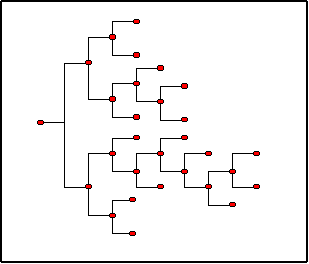
We can think of the cognitive map as a tree in which each vertex (node) represents a piece of crude knowledge and each edge (link) represents knowledge that we have already mastered and learned how to use.

Cognitive Map
Figure 1. Cognitive Map

4.4
In the graphical representation, figure 1 above, we present an example of cognitive map. This shows mastered knowledge as active nodes on the map (the coloured nodes), while all the other possible nodes, which would complete the tree, represent knowledge that at present is not in our cognitive map but could be activated through individual as well as interactive learning.

4.5
As assumed by Ancori et al., knowledge demands knowledge in order to be acquired; hence, in order to activate a new node, it would have to be directly connected to active (coloured) nodes. Moving from left to right in the cognitive map we advance from less to more specialised knowledge. This observation justifies the assumption that new nodes can only be activated (i.e. new knowledge can be acquired) if they are directly connected to active nodes.

4.6
Each agent is initially endowed with a different cognitive map, which depends upon her/his level and kind of education (measured as years of schooling and kind of school attended). Each column corresponds to a higher level of education.[5] Moreover, once education becomes specialised[6] the cognitive map will develop only in certain areas, showing more pieces of knowledge in those areas in which the agent is knowledgeable.

4.7
It is worth nothing here that in our model there is no knowledge creation, hence it is bounded to reach a stationary state in which no more knowledge exchange is possible (i.e. the CM being bounded in the number of columns and, therefore, in the number of knowledge nodes). In an ideal situation (i.e. characterised by a fully integrated system without any excluded agent or cluster of agents), the stationary state would be reached when all the agents have acquired all the possible knowledge (i.e. all cognitive maps are saturated). Nonetheless, the presence of isolated agents might generate a multiple equilibria situation. As a final note, it is important to mention that in the initial situation most knowledgeable agents will necessarily have completely saturated CM in one of the specialised areas.

4.8
The cognitive map can be formally described as: CM(X, N) where X is the set of the whole possible knowledge available (i.e. the set of vertices), and N identifies the pieces of knowledge activated (i.e. edges of the graph).

4.9
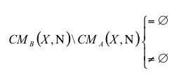
We will now explain how the process of knowledge diffusion takes place. An agent, whom we shall call A, contacts an acquaintance, B, in accordance with equation (2). Once the contact is established, the algorithm compares the two cognitive maps, subtracting the cognitive map of A from that of B. This can produce one of two possible results:[7]

eqn 4 (4)

4.10
If the difference between the two sets is a non-empty set there is possibility for interaction; if not, agent A will have no interest in interacting with agent B as there is no possible gain.

4.11
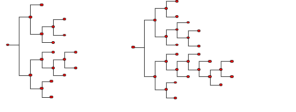
We present an example that will clarify the issue. The two maps in figure 2 represent the cognitive maps of agent A and an acquaintance, agent B. Now, let us assume that agent A contacts agent B. If we calculate the distance between the two maps we get CMB(X, N)\CMA(X, N) ≠ ∅ ( (this can be clearly observed in figure 3).

Comparing two Cognitive Maps
Agent AAgent B
Figure 2. Comparing two Cognitive Maps

4.12
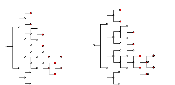
The first map below reproduces the difference between the two CMs. Once we have identified this difference, we need to identify the possible learning region where knowledge can be gained (i.e. additional nodes can be activated). To do so we recall the requirement that new knowledge has to be pegged to already existing knowledge, and thus we can cross out several of the coloured nodes in the first diagram. We conclude that the only knowledge that agent A can learn from agent B is that connected to activated nodes.

Knowledge interaction and the occurrence of learning
CMB\CMALearning Region
Figure 3. Knowledge interaction and the occurrence of learning

4.13
Defining the nodes of the learning region as Ω, then the actual learning can be expressed as , where p represents the percentage of nodes of the learning region that will be activated as a consequence of the interaction. In other words, the agent that started the interaction will activate (learn) p percent of the nodes, selected randomly (rounding always to the highest integer in the case of decimal numbers) from the learning region.[8] Since the number of nodes increases exponentially for each additional year of schooling, it implies that the higher the level of education of the interacting agents is, the higher will be the learning opportunity. This mechanism reflects the idea that the 'absorptive capacity'[9] of each agent is a positive function of her/his level of education.

4.14
In conclusion, the learning process that we have defined in this model, using a cognitive map, extends the idea developed in Morone (2001) where the author defined the level of knowledge of each agent as a function of two main variables:

eqn 5 (5)

where Ei was the level of education obtained by agent i through a formal process of individual learning, and Ii was the level of education of agent i obtained through the process of informal interactive learning (face-to-face interaction).

4.15
The latter process of learning was then defined as a function of three variables: agent i's absorptive capacity (ψi); the degree of connectivity of the network (n) within which agents interact (θn); and the average level of education of other agents eqn 5a. The knowledge function was then defined as:

eqn 6 (6)

4.16
The model developed in this paper aims to explicate, through a simulation exercise, the basic idea expressed in equation (6). We will now briefly introduce the simulation setting. Then, we will describe the dataset used to calibrate the simulation. Finally, we will present the simulation results and their implications.

* Simulation Experiments

5.1
We performed simulation experiments with a population of 232 agents allocated over a grid that resembles the map of Greater Santiago de Chile. The relative populations of each of the 34 comuna (districts) composing the grid are respected, defining a grid with different levels of density over the whole map. The grid is composed of a total of approximately 2,000 cells and has an approximate overall density of one agent per 8 cells. Each agent has a visibility ν = 2, meaning that she/he can see the two cells situated in the four cardinal directions (North, South, East and West). The initial knowledge is defined by a cognitive map constructed according to a sample drawn from Encuesta de Ocupación y Desocupación regarding years of schooling and kind of schooling, as described above.

5.2
The basic objective of the simulation experiments is to test whether knowledge diffuses homogeneously throughout the population or whether it follows some biased path generating divergence and inequality. In particular we shall investigate differences amongst the modelled districts of Santiago and amongst core and periphery areas of the geographical grid. We also examine the efficiency of the model of 'preferential acquaintance selection' with which the agents are endowed. We investigate the impact on both individual learning and on system-level knowledge diffusion by comparing with the case where there is no preferential selection.

5.3
The model was programmed in the Strictly Declarative Modelling Language (SDML) developed at the CPM (Wallis & Moss 1994) to support the modelling of social processes with multi-agent systems. The results were analysed using the graphical output capabilities of the SDML platform and the network analysis software toolkit UCINET 5.0 (Borgatti, Everett, & Freeman 1999).

Data Description

5.4
As already mentioned, the data used for the simulation are a sample of 232 agents obtained from the 1998 edition of the Encuesta de Ocupación y Desocupación of the University of Chile. This survey has been performed every year since 1957 and it covers a sample of approximately 4,000 households (with approximately 11,000 individual observations) located in the Greater Santiago area.[10] The data collected covers: demographic information; occupational information; educational information; and wage information. The 1998 survey includes additional information on effective years of working experience; number of repeated school years; kind of school attended (characterised according to the funding system[11] and the rural/urban location); parents' level of education; religion; weight; height; and finally, use (or not) of a computer at work.

5.5
The variables that are of interest to our simulation experiment are the following: district of residence, years of schooling, kind of schooling, and use of computers at work. We will use these variables to distribute agents over the geographical grid, to build the CM of each agent and to construct the cyber-network. We consider male and female agents aged between 14 and 65. We chose this range of age, as it appears to be the best representative sample of active population engaged in both interactive learning and individual learning.[12] We present below some summarising tables that describe the main statistics of our data.

Table 1: Original database

VariableNumber of Obs.MeanStd. Dev.Min.Max.
District 773218.6460210.28054134
Schooling 773210.901843.892597019
Kind 77322.5042681.40562906
Computer 77320.1462750.35340401


Table 2: Simulation sample database

VariableNumber of Obs.MeanStd. Dev.Min.Max.
District 23218.7801710.45332134
Schooling 23211.155173.758058018
Kind 2322.5775861.40900506
Computer 2320.14224140.35005201

5.6
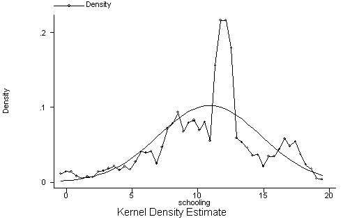
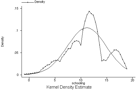
As expected, the two distributions are very similar, and in particular all the variables considered have similar standard deviations. In the following two graphs we plot the (kernel) density functions of the schooling variable for both databases (the original survey and the simulation sample).

Original database
Figure 4. Original database

Sample database
Figure 5. Sample database

5.7
No significant differences can be detected between the two distributions. Both series have one absolute maximum and two local maxima respectively at the right and the left of the absolute maximum. This indicates that the sub-sample is representative of the original sample. A more detailed analysis of the two datasets is presented in the annex.

Results and Interpretation

5.8
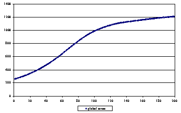
After letting agents interact for two hundred cycles we observe significant changes in the knowledge patterns. The average number of activated nodes increases substantially over the whole period, showing that the system is becoming more knowledgeable.[13] This is not surprising since agents can only increase their knowledge level (i.e. there is no loss of knowledge).

Changes in the average level of knowledge
Figure 6. Changes in the average level of knowledge

5.9
Plotting μ we can observe how first the average number of activated nodes grows very fast, then, after approximately 80-100 cycles, there is a turning point (inflection point), after which μ grows more slowly. Finally, after about 150-160 cycles, the mean curve starts levelling off, meaning that the system is reaching a stable equilibrium.[14]

5.10
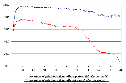
To explain these results, we first consider the dynamics underlying the structure of knowledge in the model. The number of fully saturated agents increases over time, and as agents approach this state they have a reduced potential for learning, i.e. the learning region becomes smaller. However, on the other hand, in the early stages of the simulation this region tends to widen in the CM of the majority of agents, enabling greater gains. In addition, agents will have increased opportunities to gain from interactions as CMs become more heterogeneous. For example, two agents with identical schooling will not be able to gain from an interaction in cycle 0, whereas later in the simulation they will most likely experience a small gain. This begs the question: to what extent is the observed increase in knowledge due to the widening of the learning region (i.e. the structure of the CM), and to what extent is it due to agents making better choices for interaction (i.e. the preferential model of acquaintance selection)? In the following scenario we shall test the hypothesis that the preference model for choosing among acquaintances is an efficient mechanism. To help us analyse these differences, we introduce another measurement, the 'percentage of gain interactions', which tells us how successful the learning is on an individual level. As shown in figure 7, our model of preferential selection appears to be very accurate since the percentage of gain interactions increases very sharply in the first 20 cycles and is constantly higher than 90% for more than 100 cycles. Then it starts decreasing when the system approaches a stable equilibrium.

5.11
A different picture emerges when we run the same simulation without the preferential model.[15] The number of gainful interactions is constantly smaller. Over the first 140 cycles, the simulation with preferential model is approximately 25% more efficient. Moreover, the efficiency gap (i.e. the distance in percentage gain interactions) grows bigger over the whole time span. After 140 cycles, when the model starts converging towards a stationary equilibrium, the speed at which the efficiency gap grows accelerates. In the last cycle the simulation with preferential model becomes about 70% more efficient.

5.12
The increase in the efficiency gap between the two simulations is due to the fact that agents keep meeting new acquaintances and - as the number of acquaintances grows bigger - the chances to select the right agent with whom to interact decrease. Moreover, this mechanism is accelerated after 140 cycles, as the CMs start becoming saturated: when the learning opportunities start decreasing (i.e. the learning regions become smaller) that is the moment when agents really need to know with whom it is worth interacting. Figure 7 below shows the differences between the two models so far discussed.

Percentage of gainful interactions. Studying the efficiency of the system
Figure 7. Percentage of gainful interactions. Studying the efficiency of the system

5.13
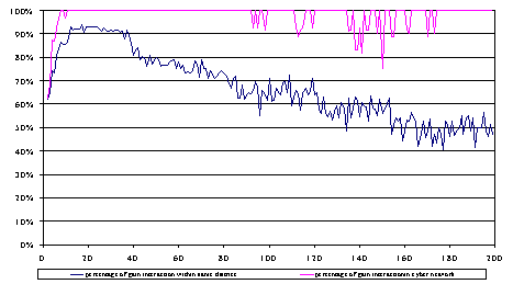
Interestingly, but not unexpectedly, most agents endowed with ICT facilities will prefer to interact with cyber-acquaintances rather than with their regular (geographical) acquaintances. As illustrated in Figure 8 below, the interactions among cyber-network members are almost always gainful, while this is not the case for interactions which take place within the same district.

Percentage of gainful interactions within districts and cyber-network
Figure 8. Percentage of gainful interactions within districts and cyber-network

5.14
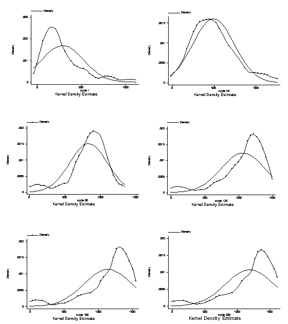
In order to investigate the distributional changes of knowledge we will start our analysis by looking at the Kernel density functions of knowledge at different moments in time. This preliminary analysis will provide a clear picture of distributional changes over time, and pave the way to a more thorough analysis of knowledge distribution.

Kernel density functions of knowledge and normal distribution
Figure 9. Kernel density functions of knowledge and normal distribution

5.15
As we can see from the figure above, the distributional changes demonstrate a clear trend: initially, there is a large majority of agents with a low level of knowledge (the mean of the distribution is in the left hand side of the first Cartesian diagram). Over time, the mean of the distribution shifts from left to right: after 40 cycles knowledge is almost normally distributed, and then it becomes skewed to the right hand side. This distributional dynamic shows clearly that the society has changed from one in which there is a majority of low knowledge agents and an 'intellectual oligarchy', to a more mature society with a majority of knowledgeable agents and some 'pockets of ignorance'. In other words, the final knowledge distribution is the mirror image of the initial one. To our understanding this change has to be interpreted as a substantial improvement in terms of knowledge distribution. This intuition is indeed corroborated by the inequality index.[16]

5.16
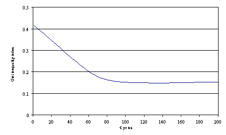
In the figure below we report the Gini index calculated over the 200 cycles of the simulation. We can observe how knowledge inequality constantly decreases over the first 100 cycles to then stabilise.

Kernel density functions of knowledge and normal distribution
Figure 10. Kernel density functions of knowledge and normal distribution

5.17
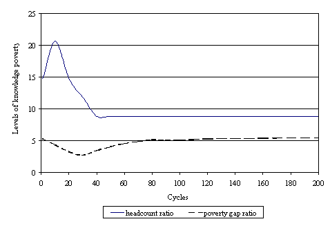
So, overall the society has quickly become less unequal as well as more knowledgeable. Nonetheless, the results indicate the occurrence of an exclusion mechanism which generates the observed 'pockets of ignorance'. In order to investigate this we need to look at poverty measures which, in this context, should be interpreted as indexes of knowledge deprivation. We calculate the first two Foster, Greer and Thorbecke indices, (i.e. the head count ratio and the poverty gap ratio) with the ignorance line[17] computed as half the median of the average level of knowledge. The difference between the two measures is that the first one is just the ratio of the number of agents having a knowledge level below the ignorance line over the total population; whereas the poverty gap ratio is intended to provide some estimate of the average knowledge shortfall from the ignorance line and thus indicates the severity of the knowledge gap rather than just the number of agents with a poor level of knowledge.

Poverty measures applied to knowledge
Figure 11. Poverty measures applied to knowledge

5.18
The figure above shows how the headcount ratio first increases and then decreases. This implies that, over the first 20 cycles, the number of agents with the level of knowledge lower than half the median is increasing. Nonetheless, those subjects are learning and getting closer to the ignorance line. We can infer this by looking at the poverty gap ratio (or knowledge gap ratio) which, over the same time-span, is decreasing. The situation reverts afterwards: now the number of agents with the level of knowledge lower than half the median is decreasing, but there is a group of agents who is falling behind, being trapped in an exclusion mechanism. In other words, the knowledge gap between this group of agents and the rest of the population grows bigger over time.

5.19
The analysis of these results becomes more revealing if we look at the simulation outcome disaggregated at district level. The geographical dimension helps in understanding the mechanisms at work that generate the observed exclusion mechanism.

5.20
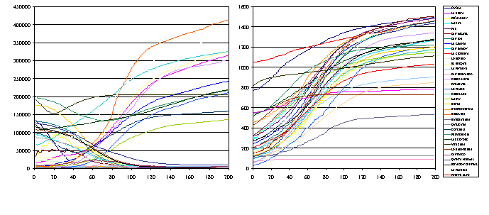
When we look at the mean and variance dynamics disaggregated at district level (see figure 9) we can draw two conclusions. First, some initially backward districts are able to catch up with the most knowledgeable ones, while others are marginalised from the learning process. Interestingly, the catching up process is not strongly correlated with the initial condition, meaning that some districts which start with a very low level of knowledge are able to reach, on average, very high levels of knowledge. At the same time, other districts which start from similar levels of initial knowledge are unable to catch up.

Changes in knowledge average and variance by districts
Variance levels by districtsMean levels by districts
Figure 12. Changes in knowledge average and variance by districts

5.21
The second conclusion is obtained when looking at the variance distribution by district. Some districts become less and less equal while others converge towards a more even equilibrium. In this case too the initial condition does not determine the twofold dynamic.

5.22
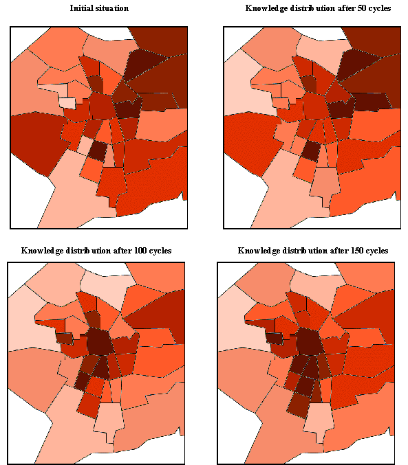
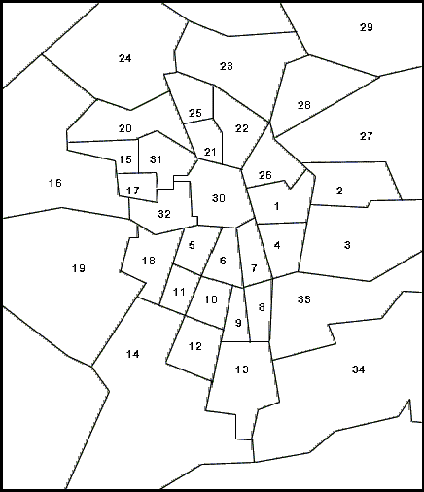
In order to understand which are the driving forces that cause only some backward districts to catch up, we need to investigate the actual geographical distribution of backward areas in the map of Greater Santiago. The four pictures reported in figure 13 below show the map of the Greater Santiago region divided into 34 districts.[18]

Changes in knowledge mean by districts
Figure 13. Changes in knowledge mean by districts

5.23
The white areas adjoining the border of the map are not included in the Santiago district. The changes in the colours show the relative changes in average level of knowledge at different stages of the simulation (absolute changes are shown in figure 12).

5.24
It is clear from the first picture that initially, the most backward districts are those situated at the western periphery of the map. In general, central districts have an initially higher mean level of knowledge. There are a number of districts in the semi-periphery also having low mean. On average, the periphery has a slightly better initial condition than the semi-periphery (this is due to the fact that we also include in the periphery rich residential neighbourhoods such as Las Condes, Lo Barnechea and Vitacura located in the north-east of the map). The situation changes over time, showing how semi-peripheral districts are able to almost catch up with central districts, while far-peripheral districts are marginalised from knowledge growth.

5.25
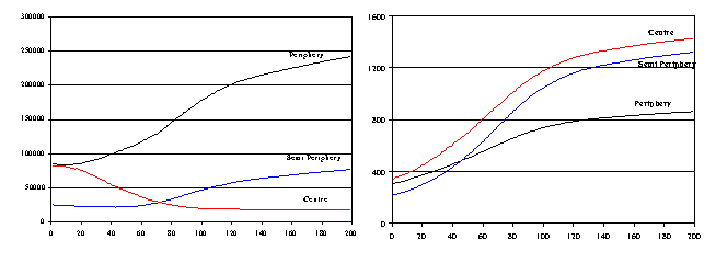
To complete our analysis, we have divided the whole region into three macro districts,[19] (i.e. centre, semi-periphery and periphery) and calculated the average level of knowledge for each macro district over time. In figure 14 below we can see the core-periphery dynamic more clearly. It emerges clearly how peripheral districts are those unable to catch up (in spite of a better initial condition with respect to semi-peripheral districts). We can therefore conclude that the geographical dimension plays a crucial role in determining the long-term equilibrium.

5.26
A further insight into this dynamic is provided by the changes in the variance calculated at macro district level (i.e. mean of district variance). The periphery and semi-periphery are the areas in which the variance grows more considerably over the long period. On the other hand, the average level of the intra-district variance decreases in the case of the central districts. Comparing with the earlier figure 12, this points out that the distribution of knowledge becomes more unequal amongst districts as well as within them. Hence, less educated agents who live in peripheral districts will be marginalised with respect to those who live in central districts, as well as with respect to the most educated agents within the peripheral macro-district.

Centre-Periphery dynamics (Average level of knowledge and Average change in knowledge variance by districts)
Average change in knowledge variance by districts Average level of knowledge by districts
Figure 14. Centre-Periphery dynamics

5.27
From these results, we can infer that the initial educational levels do not matter for those people living in central or semi-peripheral neighbourhoods to the same extent as they do for people living in peripheral areas. An intuitive explanation of this result is that if a person had not had the opportunity to acquire knowledge through individual learning but does have the chance to interact with many people, then she/he will be able to close, in the long run, the initial gap. On the other hand, if a person has a low initial level of knowledge and she/he lives in a peripheral neighbourhood, then she/he will be marginalised from society, being actually caught in a poverty trap mechanism.

Small world calculations

5.28
As discussed earlier, the simulation aims to observe the knowledge distribution dynamics as well as the network properties of the model. To tackle the issue of network properties, we follow the same methodology used in Morone and Taylor (2004). To study the network properties we calculate the average path length:

eqn 7

and the average cliquishness:

eqn 8

where X (y, z) = 1 if y and z are connected at time t (no matter whether the connection is a first generation or next generation connection), and X (y, z) = 0 otherwise.

5.29
For calculating the average path length and cliquishness of a random network, we shall use the same approximation as Watts and Strogatz (1998) that Lrandom ≅ ln N/ln n and Crandom(t) ≅ n/N, where n is the average number of connections of each agent and N is the total number of agents. The criteria for identifying the network as small worlds are that L(t) ≅ Lrandom(t) and C(t) >> Crandom(t).

5.30
We shall compare our dynamic network with a random one at different stages of the simulation to show whether or not the small worlds architecture is emerging in our system. Since the number of connections in our network is not constant (due to the mechanism by which agents make acquaintances of their acquaintances), in order to make an appropriate comparison we need to construct the random network with an equivalent number of connections. We shall, therefore, construct several random networks, one for comparison at each stage of interest of the simulation. The average path length and cliquishness will be calculated at both stages of the simulation. If, when comparisons are made with the random network, we find that the Watts-Strogatz criteria are observed, this will be evidence to suggest that a small worlds network structure is emergent from our model.

5.31
In Table 3 below we present our results for the small world calculations. Looking at this figure we observe that L (average path length) is substantially stationary, while on the other hand, C (average cliquishness) first decreases and then increases again. The initial situation is definitely a small world with L(t) ≅ Lrandom(t) and C(t) >> Crandom(t) (i.e. where short average path length and high degree of cliquishness coexist). Then, after fifty cycles, the architecture of the network changes slightly (with a cliquishness which decreases by more than 60%). After another 50 cycles, the network evolves again into a small world and remains stable until the end of the simulation.


Table 3: Small world calculation results

CL
Simulation ResultsCycle 10.43962.1727
Cycle 500.14252.3082
Cycle 1000.26612.9281
Cycle 1500.28533.2699
Cycle 2000.25782.9669
Random NetworkCycle 10.03882.4789
Cycle 500.03452.6193
Cycle 1000.03452.6193
Cycle 1500.03022.7991
Cycle 2000.03022.7991

5.32
From the results obtained we can conclude that the network structure of the model evolves over time. This dynamic process is particularly interesting since it shows that the network evolves into a very efficient structure (i.e. small world), by means of an individual learning process, which takes place through the model of preferential acquaintance selection described above. In other words, what is efficient for the individual is also efficient for the network as a whole.

* Conclusion

6.1
In this paper we have modelled the dynamic process of knowledge diffusion, where knowledge is structured non-linearly as a cognitive map. The process through which agents interact allows each agent to learn from her/his acquaintances and to increase her/his knowledge in the learning region of the CM. Whether or not the interaction is gainful will depend upon the precise structure of that knowledge. The simulation was calibrated on the Greater Santiago region, using a sub-sample of the original database obtained from the Encuesta de Ocupación y Desocupación collected by the University of Chile for the year 1998.

6.2
We have also studied the network properties of the model over the whole simulation. We observed how the network architecture of the model changed over time, evolving into a very efficient one (i.e. small-world) by means of an individual learning process, which takes place through the model of preferential acquaintance selection.

6.3
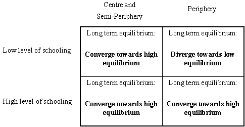
The results concerning the knowledge diffusion process are very interesting: in presence of high level of (knowledge) inequality there is a high risk of exclusion for those people initially endowed with low level of education. Moreover, we studied the spatial dimension of the exclusion process, finding that the ignorance trap mechanism is more likely to take place if an initial situation of low level of knowledge is coupled with geographical exclusion. In other words, those people who start with a high level of individual learning (i.e. schooling) will always be able to escape from the ignorance trap mechanism, while more backward people might be trapped if their low level of knowledge is cumulated with geographical exclusion. To summarise, each agent can find her/himself in one of the following four situations:

Possible long-term equilibria
Figure 15. Possible long-term equilibria

6.4
These findings are extremely important from a policy prescription perspective. In the light of these new findings, two possible policy actions could help to avoid the occurrence of an ignorance trap: the policy maker could increase the level of education of more backward and marginalised peoples, and/or reduce the geographical gap between centre and periphery. This latter policy could be implemented through the development of infrastructure bridging the centre-periphery distance, as well as through the development of ICT. In other words, the exclusion risk could be minimised through the development of a more comprehensive cyber-network, so that also peripheral agents will have the same opportunity to interact with central and semi-peripheral agents.

* Annex


Table A1: Schooling distribution, original sample

SchoolingFreq.PercentCum.
01441.861.86
1260.342.2
2680.883.08
31341.734.81
41592.066.87
51271.648.51
63905.0413.55
71572.0315.58
87249.3624.95
95537.1532.1
106258.0840.18
114806.2146.39
12215527.8774.26
134155.3779.63
143124.0483.67
152052.6586.32
162893.7490.05
174916.3596.4
182312.9999.39
19470.61100
Total7732100


Table A2: Schooling distribution, simulation sample

SchoolingFreq.PercentCum.
010.430.43
220.861.29
320.862.16
493.886.03
552.168.19
6104.3112.5
762.5915.09
8208.6223.71
9166.930.6
10208.6239.22
11114.7443.97
126829.3173.28
13125.1778.45
1462.5981.03
1552.1683.19
16125.1788.36
17198.1996.55
1883.45100
Total232100


Table A3: Geographical distribution, original sample

DistrictFreq.PercentCum.
12533.273.27
2981.274.54
33774.889.42
41952.5211.94
51992.5714.51
6861.1115.62
71982.5618.18
81762.2820.46
91772.2922.75
101451.8824.62
112112.7327.35
122903.7531.1
133053.9435.05
142703.4938.54
152423.1341.67
162833.6645.33
171531.9847.31
181381.7849.09
195156.6655.76
201562.0257.77
21861.1158.89
222613.3862.26
23730.9463.2
241031.3364.54
252082.6967.23
261291.6768.9
274666.0374.92
281511.9576.88
2977177.87
303073.9781.84
311802.3384.17
322022.6186.78
335296.8493.62
344936.38100
Total7732100


Table A4: Geographical distribution, simulation sample

DistrictFreq.PercentCum.
152.162.16
220.863.02
3208.6211.64
431.2912.93
583.4516.38
620.8617.24
752.1619.4
862.5921.98
973.0225
1010.4325.43
1183.4528.88
1293.8832.76
1362.5935.34
1462.5937.93
1552.1640.09
1662.5942.67
1710.4343.1
1852.1645.26
19156.4751.72
20114.7456.47
2131.2957.76
2252.1659.91
2331.2961.21
2441.7262.93
2583.4566.38
2641.7268.1
27156.4774.57
2862.5977.16
2931.2978.45
3083.4581.9
3162.5984.48
3262.5987.07
33135.692.67
34177.33100
Total232100


Table A5: Distribution of kind of school, original sample

KindFreq.PercentCum.
01391.81.8
1177522.9624.75
2299538.7463.49
3102913.3176.8
44746.1382.93
5130516.8899.81
6150.19100
Total7732100


Table A6: Distribution of kind of school, simulation sample

KindFreq.PercentCum.
010.430.43
15322.8423.28
28938.3661.64
33314.2275.86
4135.681.47
54218.199.57
610.43100
Total232100


Table A7: Distribution of use of computer at work, original sample

ComputerFreq.PercentCum.
0660185.3785.37
1113114.63100
Total7732100


Table A8: Distribution of use of computer at work, simulation sample

ComputerFreq.PercentCum.
019985.7885.78
13314.22100
Total232100

Map of Greater Santiago Region and District Codes

DistrictCode
ÑUÑOA1
LA REINA2
PEÑALOLEN3
MACUL4
PAC5
SAN MIGUEL6
SAN JOA7
LA GRANJA8
SAN RAMON9
LA CISTERNA10
LO ESPEJO11
EL BOSQUE12
LA PINTANA13
SAN BERNARDO14
CERRO NAVIA15
PUDAHUEL16
LO PRADO17
CERRILLOS18
MAIPU19
RENCA20
INDEPENDENCIA21
RECOLETA22
HUECHURABA23
QUILICURA24
CONCHALI25
PROVIDENCIA26
LAS CONDES27
VITACURA28
LO BARNECHEA29
SANTIAGO30
QUINTA NORMAL31
ESTACION CENTRAL32
LA FLORIDA33
PUENTE ALTO34

Macro-districts Composition:
Centre: 1, 4, 5, 6, 7, 21, 26, 30, 31, 32;
Semi-periphery: 8, 9, 10, 11, 12, 13, 15, 17, 18, 20, 22, 25;
Periphery: 2, 3, 14, 16, 19, 23, 24, 27, 28, 29, 33, 34.
Figure A1. Map of Greater Santiago Region and District Codes


* Acknowledgements

The authors are grateful to Nick von Tunzelmann, Scott Moss, Robin Cowan and Ed Steinmueller for helpful comments in different stages of the work. The usual disclaimers apply.

* Notes

1 See among others: Beyer 2000; Morone 2001.

2 See, among others, Ellison (1993, 2000), Anderlini and Ianni (1996), Berninghaus and Schwalbe (1996), Goyal (1996), Akerlof (1997), Watts (2001).

3 An intuitive example would be that of a student who stops interacting with her/his teacher when she/he feels that she/he has nothing to learn from the interaction, or when her/his knowledge surpasses that of her/his teacher. Another example could be that of two equally educated agents who might stop communicating when they become specialised in two very different areas, so no shared interest remains.

4 In this way we assume that agents are constrained by 'bounded rationality' in the sense that they respond to utility signals. This does not mean that they maximise utility (Katz 2001).

5 Moving from left to right, each pair of years of schooling corresponds to a complete column activated. We set the initial level of education (0 to 2 years of schooling) as three full columns activated (with the third column containing four nodes), then additional pairs of years of schooling correspond to an additional column in the cognitive map.

6 After the eighth year of schooling students choose to specialise either in humanistic-scientific general education or technical-professional education.

7 We define the cognitive map only as a function of X and N because at this stage we are not interested in the depth of knowledge.

8 In the simulation model p is set equal to 0.1.

9 We refer explicitly to the work of Cohen and Levinthal (1989) on returns from R&D. The concept of individual absorptive capacity was already developed in Morone (2001).

10 This region, called Región Metropolitana, includes 42% of the economically active national population (see: Bravo et al. 1999:7).

11 Chilean schools can be entirely funded by the government, partially funded by the government or entirely private.

12 Agents younger than 14 years old are probably engaged mainly in individual learning as schooling represent a major part of their life, while people over 65 are probably less likely to be involved in knowledge exchange processes (because they are already too wise!).

13 Given the structure of knowledge expressed by the cognitive map, we calculate changes in knowledge based on the total number of activated nodes for each agent.

14 Longer simulations show how the curve completely levels off, meaning that the system reaches a long-run stable equilibrium.

15 The only change introduced was in the preferential selection: the value τi defined in equation (3) was not updated so it remained equal to 1. No acquaintances were dropped. Apart from that the two simulations here compared are identical.

16 We studied distributional changes by means of inequality and poverty measures used typically in income distribution analysis. We did so because we are interested in studying the distributional properties of the model as well as its network and efficiency properties.

17 We call the ignorance line what is usually called the poverty line.

18 A detailed map with the district codes is reproduced in the annex.

19 A detailed description of each macro-district composition is reproduced in the annex.


* References

ABRAMOVITZ, Moses (1989), Thinking about growth, Cambridge University Press, 1989.

AKERLOF, G. (1997), "Social Distance and Social Decisions", Econometrica, 65: 1005-1027.

ANCORI, B., A. Bureth, et al. (2000), "The Economics of Knowledge: the Debate About Codification and Tacit knowledge", Industrial and Corporate Change, 9, (2): 255-287.

ANDERLINI, L. and A. Ianni (1996), "Path Dependence and Learning from Neighbours", Games and Economic Behaviour, 13: 141-177.

BALA, V. and S. Goyal (1995), "A Theory of Learning with Heterogeneous Agents", International Economic Review, 36(2): 303-323.

BALA, V. and S. Goyal (1998), "Learning from Neighbours", Review of Economic Studies, 65: 595-621.

BÉNABOU, R. (1993), "Working of a City: Location Education and Production", Quarterly Journal of Economics, 58: 619-652.

BERNINGHAUS, S. and U. Schwalbe (1996), "Evolution, Interaction, and Nash Equilibria", Journal of Economic Behaviours and Organization, 29: 57-85.

BEYER, H.(2000), "Education and Income Inequality: A New Look", Estudios Publicos, 77.

BORGATTI,S.P., M.G. Everett, and L.C. Freeman, (1999), UCINET 5.0 Version 1.00. Natick: Analytic Technologies.

BRAVO, D., D. Contreras, Madrano (1999), "The Return to Computer in Chile: Does it Change after Controlling by Skill Bias? ", mimeo, Department of Economics, University of Chile.

BROCK, W. and S. Durlauf (1995), "Discrete Choice with Social InteractionI:Theory" NBER Working Paper, 5291.

CHWE, M. S-Y. (2000), "Communication and Coordination in Social networks", Review of Economic Studies, 67: 1-16.

COHEN, W. M. and D. A. Levinthal (1989), "Innovation and Learning: The Two Faces of R&D", The Economic Journal, 99(September): 569-596.

COWAN, R. and N. Jonard (1999), "Network Structure and the Diffusion of Knowledge", MERIT Working Papers, 99-028.

DURLAUF, S. (1996), "Neighborhood Feedbacks, Endogenous Stratification, and Income Inequality", in: W. Barnett, G. Gandolfo and C. Hillinger (ed), Dynamic Disequilibrium Modelling, Cambridge, Cambridge University Press.

ELLISON, G. (1993), "Learning, Local Interaction, and Coordination", Econometrica, 61: 1047-1071.

ELLISON, G. (2000), "Basins and Attraction, Long Run Stochastic Ability and the Speed of Step-by-Step Evolution", Review of Economic Studies, 67: 17-45.

ELLISON, G. and D. Fudenberg (1993), "Rules of Thumb of Social Learning", The Journal of Political Economy, 101(4): 612-43.

ELLISON, G. and D. Fudenberg (1995), "Word-of-Mouth Communication and Social Learning", Quarterly Journal of Economics, 110(1): 93-125.

GLAESER, E. L., B. Sacerdote, and P. Scheinkman (1996), "Crime and Social Interactions" Quarterly Journal of Economics, 111: 507-548.

GOYAL S. (1996), "Interaction Structure and Social Change", Journal of Institutional and Theoretical Economics, 152: 472-494.

JOVANOVIC, B. and R. Rob (1989), "The growth and diffusion of Knowledge", Review of Economic Studies, 56(198-9): 569-82.

KATZ, J. (2001), "Structural Reforms and Technological Behaviour. The Sources and Nature of Technological Change in Latin America in the 1990s", Research Policy, 30: 1-19.

KIEFER, N. (1989), "A Value Function Arising in Economics of Information", Journal of Economic Dynamics and Control, 7: 331-337.

MORONE P. (2001), "The Two Faces of Knowledge Diffusion: the Chilean Case", Universidad de Chile, Departamento de Economia, Working Paper, 178.

MORONE, P. and R. Taylor (2004), "Knowledge Diffusion Dynamics of Face-to-Face Interactions", Journal of Evolutionary Economics, forthcoming.

MORRIS, S. (2000), "Contagion", Review of Economic Studies, 67: 57-68.

WALLIS, S., and S. Moss (1994), Efficient Forward Chaining for Declarative Rules in a Multi-Agent Modelling Language, available online at: http://www.cpm.mmu.ac.uk/cpmreps

WATTS, A. (2001), "A Dynamic Model of Network Formation", Games and Economic Behaviours, 34: 331-341.

WATTS, D. and S. Strogatz (1998), "Collective Dynamics of Small-World Networks", Letters to Nature, 393, June: 440-442.

WILSON, R. J. and J. J. Watkins (1990), Graphs: An Introductory Approach, Wiley: New York.

----

ButtonReturn to Contents of this issue

© Copyright Journal of Artificial Societies and Social Simulation, [2004]