Ioannis D Katerelos and Andreas G Koulouris (2004)

Seeking Equilibrium Leads to Chaos: Multiple Equilibria Regulation Model

Journal of Artificial Societies and Social Simulation vol. 7, no. 2
<https://www.jasss.org/7/2/4.html>

To cite articles published in the Journal of Artificial Societies and Social Simulation, reference the above information and include paragraph numbers if necessary

Received: 16-Nov-2003    Accepted: 24-Feb-2004    Published: 31-Mar-2004

Abstract

In this paper, we shall present a model of opinion dynamics called Multiple Equilibria Regulation (MER) Model which, concerning social equilibrium, is based on the Bounded Confidence (BC) Models procedures and, it takes under consideration an agents internal ("intra-individual") regulation structure among different opinions regarding the same social issue. First, we give a detailed description of the model and define its parameters. Then, we explore this nonlinear model by a series of computer simulations for a variety of parameter values. Next, we examine under what conditions the model exhibits sensitive dependence on initial conditions and, finally, we calculate the Lyapunov Exponents and the Information Entropy. Our results show that for certain parameter values, the system exhibits sensitivity of final state to initial state, thus it is chaotic (deterministic and unpredictable). Hence, by combining two psychosocial principles that both tend to certainty (stability) we obtain an uncertainty (unpredictability) concerning the outcome of the system.

Keywords:

Opinion dynamics, social, intra-individual, equilibrium, sensitivity to initial conditions, unpredictability, transient chaos

Introduction

1.1

In many ways, social systems are conceptually intended to seek equilibrium. Following Sorokin (1927), Walter Buckley (1967) describes the origin of social physics (in the 17^th century) like a central consideration of a person or a society to be an elaborate machine. Vilfredo Pareto (1916/1935) supplemented this mechanical model with the idea of equilibrium. In his concept of equilibrium, "any moderate changes in the elements or their interrelationships (of a system) away from the equilibrium position are counterbalanced by changes tending to restore it" (p.9). This concept of systemic equilibrium was taken over almost unchanged by many sociologists following Pareto, especially by Talcott Parsons (Buckley 1967; Parsons 1977).

1.2

Such a point of view can be found modeled in social simulations' bibliography (Hegselmann & Krause 2002) under the general title "Bounded Confidence (BC) Model" ^[1]. This model assumes that an agent who trusts in the opinions of a selected group of agents does aggregate these opinions by adopting their average. The analysis is mainly centered in categorizing the system's final states according to the number of emergent clusters: thus, if one group is formed then we classify this case as consensus, if two clusters appear then it is polarisation and, finally, if more than two groups are formed then we have opinions' fragmentation. The BC model implements the principle of social equilibrium: in socio-psychological terms, this means that every conformity model (expressed as "averaged" opinions between agents) leads the system in a form of equilibrium alias a stable and stagnant position. Empirically, although our agents seem to aspire equilibrium as an aim, it can be acknowledged that no "real" social system ever attains this kind of configuration.

1.3

In addition, admitting such models as close to "reality" implies the acceptance of the postulate that each attitude concerning a given social issue at stake can be contained and expressed by one and only one "global" opinion. Socio-psychologists tend to consider that, in place of a scientific type of truths which should follow logic rules, social thought can be much more ambiguous: opposing points of view can be formulated with equal reasonableness (Perelman 1979; Billig 1991). Thus, a proposition and its opposite can both appear reasonable and equally attractive to a person. At a cognitive level, a person "knows" both the proposition and its opposite, but an internal mechanism of regulation, a structural configuration, is responsible for adjusting and regulating their conflictual^[2] co-existence. Consequently, in a typical situation, a person holds opinions that are (socially) viewed as "opposites".

1.4

We can say that, in a field theory tradition (Lewin 1936), both A and B may be components of the same whole concerning the given social issue, in spite of their opposition. Therefore, we suppose that all components of the same set (if we consider it as finite) are in a constant inter-relation^[3] and the structure between them regulates the stability of the whole. Thus, we can reasonably assume that each time a social issue is at stake, a double (at least) negotiation takes place: when a person discusses this issue with others, automatically and inevitably s/he discusses about both opinions A and B. If both opinions have the same magnitude then, this configuration is unstable and, hence, the person tends to decrease the amount of produced cognitive dissonance (Festinger 1957). In other words, one must preserve some kind of equilibrium in his or her thoughts and discourse: a structure (socially shared and constructed) is regulating the variety of opinions, which exists in every day's social exchange. Equilibrium, on the other hand, is not achievable until all relevant opinions' dynamics obey a prescriptive/deontic way of co-existence.

1.5

In terms of the person's cognitive system, therefore, there is a continual striving for consistency, a push towards congruent, harmonious, fitting relationships between cognitive elements or between thoughts, opinions and actions that make up a structure of cognitions about some object or event. Thus, when inconsistency is felt by an individual, some psychological tension is presumably set up by motivating his behavior in the direction of reducing this inconsistency and re-establishing harmony. The cognitive process constantly strives toward cognitive balance. Although it is generally true that a person tends to make various aspects of his cognitive functioning consistent with one another, it cannot be said that any individual cognitive system achieve ever a state of perfect consistency. Nevertheless, even if there are some limits to this principle, however, it has been proven a powerful predictive tool.

1.6

In the following paragraphs, we present a model of opinion dynamics called the Multiple Equilibria Regulation (MER) Model, which, concerning social equilibrium, is based on the BC Model's procedures and it takes under consideration an internal (see "intra-individual") dissonance regulation structure between different opinions regarding the same social issue. In section 2 we give a more detailed description of the model and define its parameters, in section 3 we explore this nonlinear model by a series of computer simulations for a variety of parameter values, in section 4 we examine under what conditions the model exhibits sensitive dependence on initial condition and we calculate the Lyapunov Exponents (4.8) and the Information Entropy (4.13) in order to verify the sensitivity and the chaotic behavior of the model.

The Multiple Equilibria Regulation (MER) Model

2.1

Suppose that we have N agents and a social issue, which is at stake. Among them, for reasons of simplicity, a double opinion formation process is taking place: this means that every agent holds two opinions relevant to the given issue. We also define a structure that regulates opinions' inter-relations. In this simplified form of two opinions (A and B), opinion A goes the other direction of opinion B (do not "go together", Flament 1981).

2.2

As an example^[4], a person can hold an opinion A regarding the possible purchase of Company X's stocks. Opinion A can be expressed in a sentence-like form: "I want high short-term profits!" On the other hand, an opinion B "opposite" to A, might be expressed like: "I want a secure investment!" Everybody knows that seeking high short-term profits in the Stock Exchange Market implies high risk of losing money. The given person negotiates both opinions simultaneously and, s/he complies with the principle of social equilibrium by changing^[5] his opinions according to his group of influence. However, just after the negotiation of opinions A and B with others is interrupted, a person needs to look "inside" her/himself, in his cognitive world, and ascertain that s/he is internally consistent. If the outcome of the social negotiation of both opinions does not disturb his internal cognitive balance (Heider 1946), then s/he accepts this situation as it is. When s/he realizes that, by means of social interaction, s/he has arrived at a point where s/he is changing both opinions in the same way, s/he feels the dissonance caused by the cognitive contradiction asserted. In our case, "By doing this, I consent more to the proposition that 'I want high short-term profits' and, simultaneously, I am more persuaded that 'I want a secure investment' ".

2.3

Since the person is obliged to balance, we must define an algorithm of regulation. We assume first that the person examines the magnitude of change of both opinions. Then, by focusing on maximum change, s/he decides to "accept" the opinion that suffered the maximum change, and s/he "rejects" the minor change. This magnitude of maximum change is considered as a "correction" for adjusting the other opinion and, by seeking intra-individual stability, one adds or subtracts this difference (multiplied by the intra-regulation factor Ψ, as will be explained later) by conforming the direction of change according to the given structure: if "High profits" is changed in maximum manner, then "security (low risk)" should be changed by the same magnitude but in the opposite direction. Hence, our subject combined expression can take this form: "Since, I've shifted positively for 'high short-term profit' then, in order to keep internal equilibrium, I 'must' diminish accordingly my belief that I'm going to lose my money in a high risk investment...". Therefore, by this simplified process, one seeks intra-individual equilibrium^[6]. It is clear that we define the dynamics of the system as something "on the move": each agent takes under consideration only the changes obtained by means of social interaction. In this point of view (a "rhinoceros view^[7]"), agents are conscious only of the changes effectuated and not of the values themselves, which can be considered as (static) products of this process. We must say that, in any way, these static values do not remain "static" long enough to be observed, our model is essentially dynamic.

2.4

Nevertheless, it is evident that for all dissonances one cannot be sure that the same rule will be followed. In other words, adding or subtracting the "difference" as it is, implies that we accord the same change in the opposite opinion. This means that the influence exerted from one opinion to the other, maintains a proportion of 1 to 1: the same change having derived from one opinion is used to regulate the other. In a more general case, we add or subtract the difference multiplied by an intra-regulation factor Ψ. Obviously, Ψ can take values between 0 (no inter-opinion regulation, the tendency to intra-individual equilibrium is absent) and infinity. Nevertheless, Ψ is considered to be limited theoretically^[8]. For instance, for Ψ = 1, we correct the dissonant opinion by adding or subtracting exactly the magnitude of maximal difference. For Ψ = 2, we correct the dissonant opinion by doubling the maximal difference and for Ψ = 0.5 we correct by adding or subtracting half of the maximal difference. It is clear that Ψ coupled with the bound of confidence ε (as defined in BC Model) are the key parameters of our model.

2.5

In order to clarify the procedure we give an example. We set ε = 0.1 and Ψ = 0.5 (the parameter values of MER model). We consider 100 agents and every one is assigned with two numbers belonging to the interval [0,1], each number denoting an opinion. The distribution of initial opinions is random (random initial profile). Each agent is aware of the opinions of all other agents. As defined in the BC Model, an agent i takes only those agents j into account whose opinions differ from his own no more than the confidence level (the bound of confidence) ε = 0.1. Suppose that agent's i opinion 1 equals 0.8 and opinion 2 equals 0.4. Agent i knows that a subset of the agents have opinion 1 that lay into the confidence interval [0.7, 0.9] and calculates the average (mean value) of their opinion 1, lets say that this value equals 0.86. This means that according to the influence posed on her/him, s/he has to shift his opinion 1 positively to the new value. Thus, s/he "sees" his opinion 1 augmenting for 0.86 - 0.8 = 0.06. The same procedure is followed concerning opinion 2: agent i also "realizes" that some agents' opinion 2 lay into his confidence interval [0.3, 0.5] and calculates the average (mean value) of their opinion 2; let's say that this value equals 0.42. This means that according to the influence posed on her/him by his social environment s/he has to change his opinion 2 to the new value, so s/he shifts positively for 0.42 -0.4 = 0.02. Up to now, we have two BC Model simulations running simultaneously but remaining unrelated.

2.6

As described previously, agent i confronts a dilemma. If s/he accepts both shifts as they are, s/he will be inconsistent according to the rule presented by the balanced structure. So, s/he focuses on the opinion which has the maximal shift, s/he accepts this value and s/he decides to regulate the other opinion in relation with it. The biggest change (influence) in agent i occurred in opinion 1. New opinion 1 (Op. 1= 0.86) is then accepted while opinion 2 is regulated internally in order to attain equilibrium and moves to the opposite direction from opinion 1. The new-formed opinion 2 that equaled 0.42 is not accepted and the agent regulates it by moving his opinion 2 from 0.42 downwards for 0.06 · Ψ = 0.06 · 0.5 = 0.03. Finally, s/he sets opinion 2 to 0.42 - 0.03 = 0.39. A detailed mathematical description of the whole process can be found in Appendix A.

Keeping the system constrained in [0,1]: the Rescale Process

2.7

Although, for all simulations we have done up to now, the system reaches a final steady state and thus remains bounded (no opinion escapes to infinity), after iterating, some opinions become bigger than 1 or lesser than 0. In order to keep opinions into the original interval [0,1] and, at the same time, not to change the dynamical behavior of the system we apply a procedure we call "rescale" ^[9].

2.8

If, for some iteration, in case that even one opinion of an agent escapes the interval [0,1], we rescale all opinions as follow: we calculate the maximum=max and the minimum=min of opinions 1 and 2 of all agents. If min is negative, then we translate all opinions upwards by subtracting min (min is negative), so in fact we augment all opinions and make them positive or zero. Then we divide all opinions by a scaling factor, which is the range of their values.

2.9

All options of rescale are described in table 1.

Table 1: Rescale process: scaling factor according to the range of values of opinions 1 and 2
Value's range	Scaling factor
max>=1 and min<0	max-min
max>1 and min>=0	max
max<=1 and min<0	1-min
max<=1 and min>=0	1

2.10

Pseudocode of the actions performed at each time step (iteration) including the rescale process can be found in Appendix B.

Simulations

3.1

According to Hegselmann & Krause (2002), the study of BC Model can give birth to a typology of final stable configurations. As dependent to the magnitude of bound used, the BC Model usually ends up with three possible final states: consensus, polarization and fragmentation. These states occur respectively in three bound's intervals: ε around and above 0.3, ε smaller than 0.3 and bigger than 0.1 and, finally, ε around 0.1 and smaller. This is to say that in each state described above we have a different segmentation of the agent's corpus: consensus means that all agents reach the same final opinion, polarization signifies those agents' population that end up divided into two clusters and, fragmentation stands for a configuration of more than two clusters of opinions.

3.2

In our primary exploration of the MER Model, we have chosen three bounds of confidence according to the aforementioned typology of BC Model: 0.1, 0.2 and 0.3. On the other hand, a second parameter, the intra-regulation factor Ψ, quantifies interior balance correction factor: we expect different output configurations with respect to the magnitude of Ψ. We have selected three values: 0.5, 1 and 1.5:

• Ψ = 0.5 stands for a type of agent which under-correct their opinions and, hence, they underestimate the importance of their internal balance. These agents seem to ascribe a minor importance to intra-individual equilibrium.
• Ψ = 1 signifies that agents correct their opinions in an equal manner. This type of agent's internal structure means that an equal importance has been given in both social and intra-individual equilibrium.
• Ψ= 1.5 means that our agents over-correct their opinions and, thus, they overestimate the importance of their internal balance. These agents seem to ascribe a minor importance to social equilibrium.

3.3

In tables 2, 3 and 4 one can see results for all possible combinations between the selected ε and Ψ values: 9 cases in total. Since the simulation of MER Model implies the interaction of two opinions of the agents synchronously, we present both opinions' dynamic: in each cell of the table, one can find the trajectories of opinion 1 or 2.

Ψ = 0.5 ε Opinion 1 Opinion 2 0.1 0.2 0.3

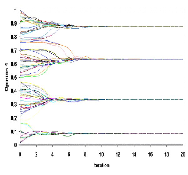
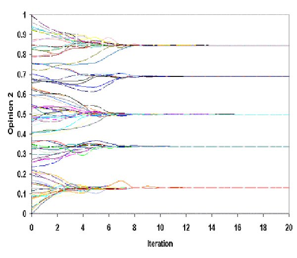
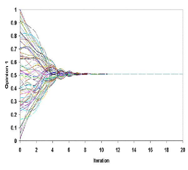
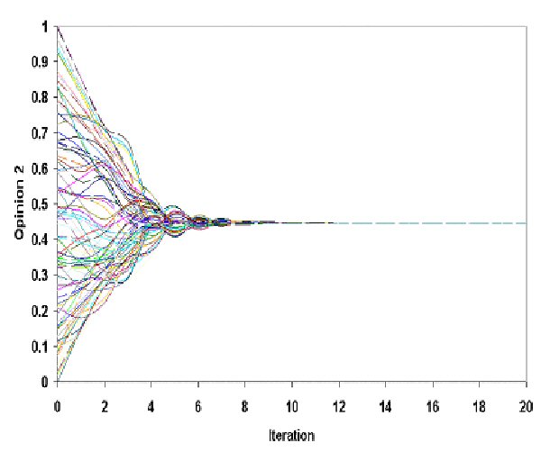
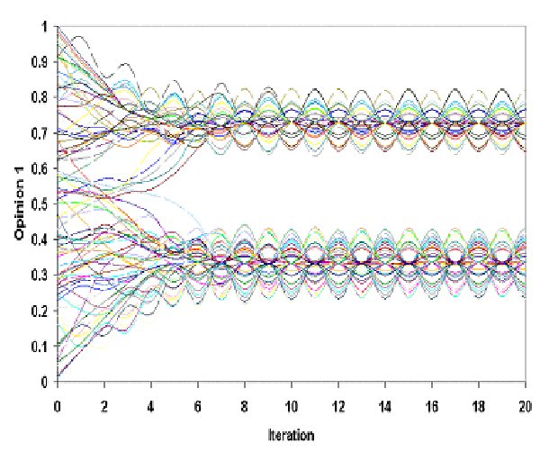
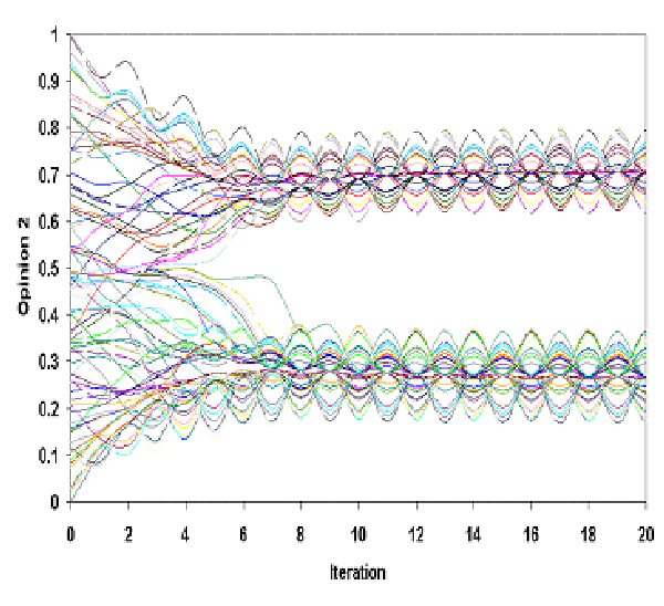
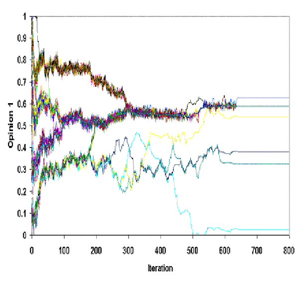
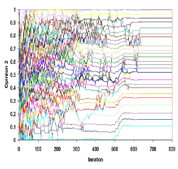
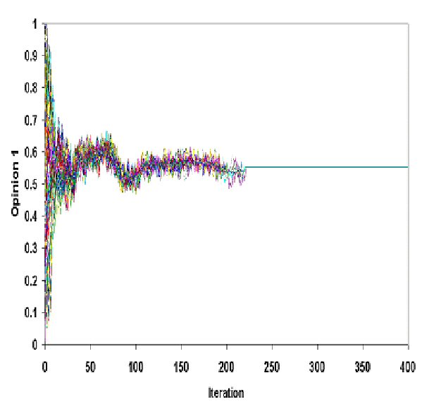
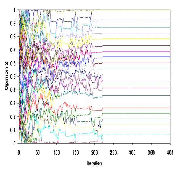
Table 2. Simulation of MER Model for Ψ = 0.5 and three values of ε

Ψ = 1 ε Opinion 1 Opinion 2 0.1 0.2 0.3

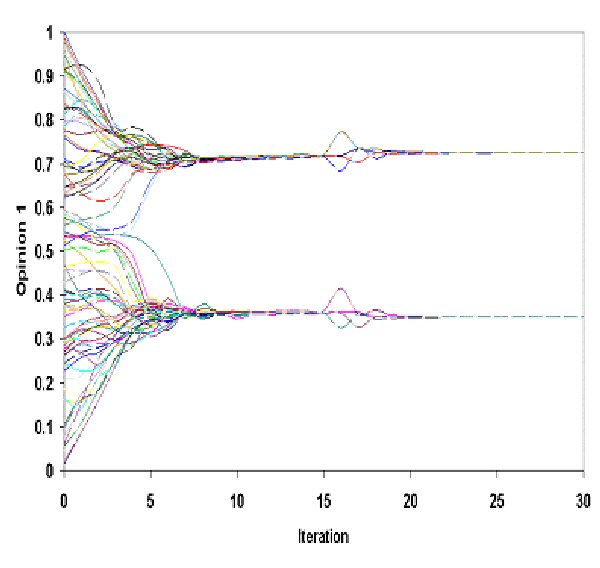
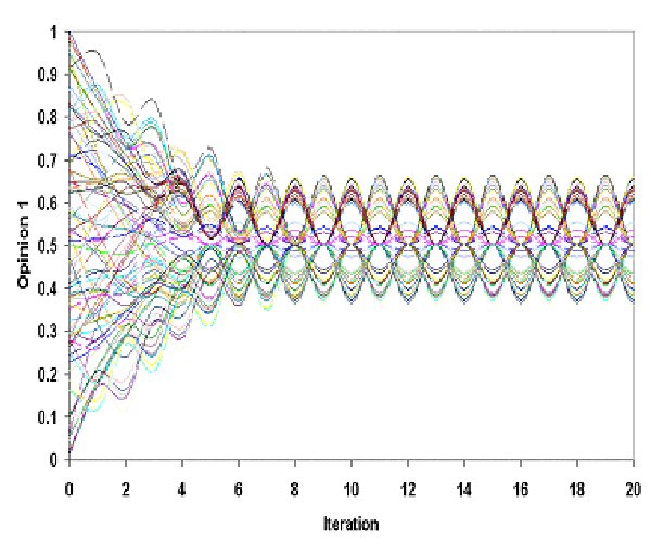
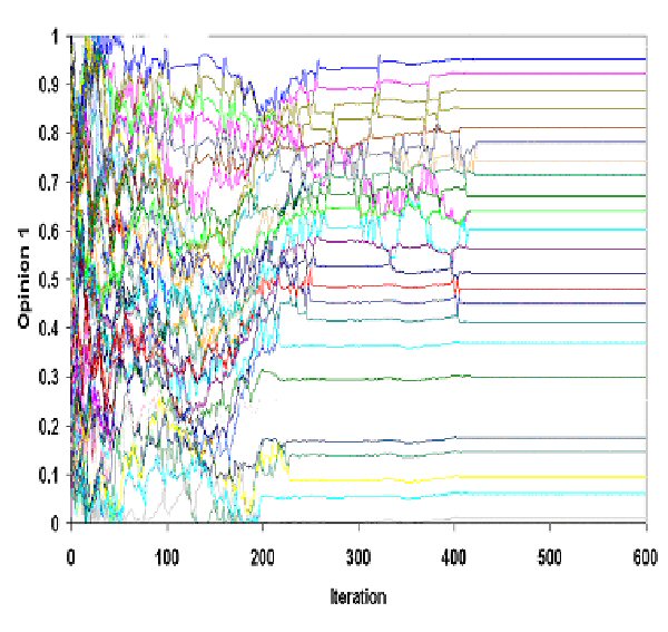
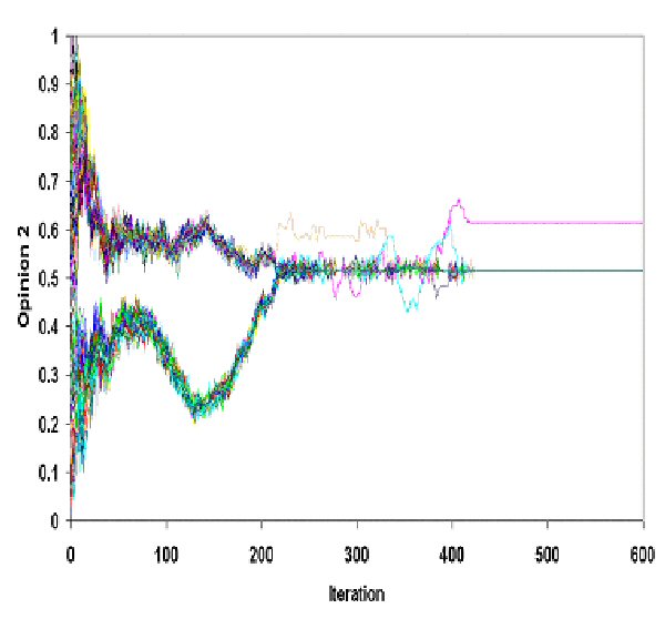
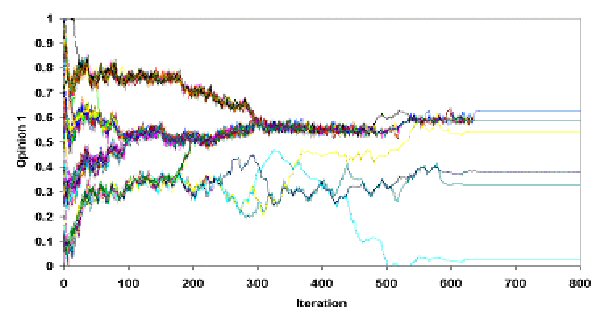
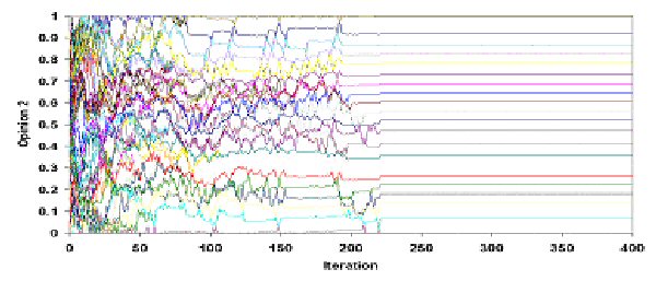
Table 3. Simulation of MER Model for Ψ = 1 and three values of ε

Ψ = 1.5 ε Opinion 1 Opinion 2 0.1 0.2 0.3

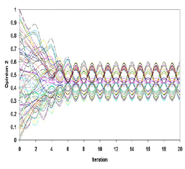
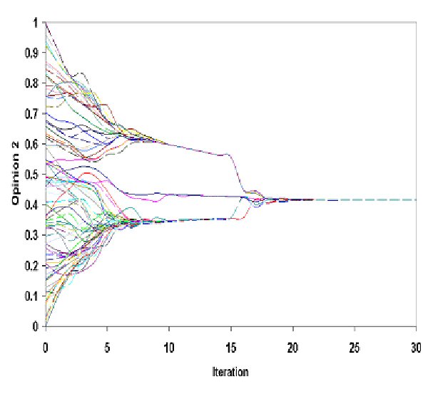
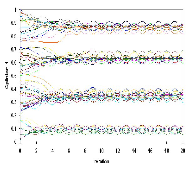
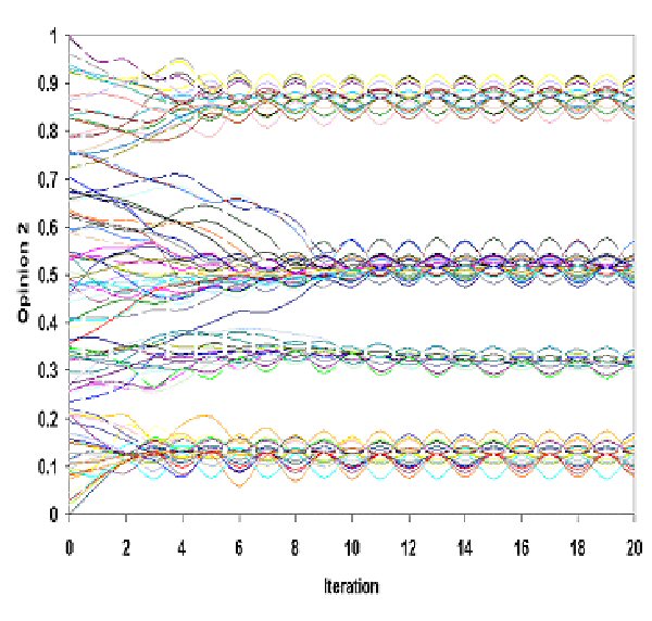
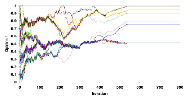
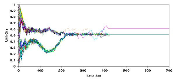
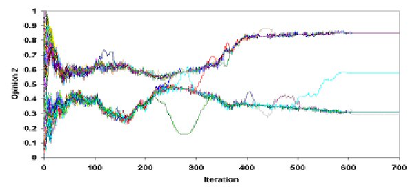
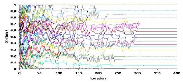
Table 4. Simulation of MER Model for Ψ = 1.5 and three values of ε

3.4

In table 2 (Ψ = 0.5), we observe that dynamical behavior of both opinions seem to be similar to those produced by the BC Model. Nevertheless, we note that in MER Model, agents seem to have many ups and downs before they reach their final steady state, thus trajectories are far more "turbulent" than those of the agents in the traditional BC Model (compare with Figure 2 and 4 in Hegselmann & Krause 2002). Although this is a qualitative difference, it is striking that even a rather small Ψ tends to destabilize the smooth trajectories found in BC Model and seems to perturb them in their way of attaining social equilibrium.

3.5

In table 3 (Ψ = 1), where both tendencies (towards social and intra-individual equilibrium) are of equal strength, all final states (for both opinions) are periodic. This means that, our agents oscillate in a periodic way, by matching their dissonant opinions. In this case, the agents seem to adopt the more stable form of movement: their dynamical behavior, by avoiding a motionlessness state (presented when Ψ = 0.5), is an eternal but "harmonious" motion. In this way, the agents are not stagnant, which is unlikely in an empirical reality and, on the other hand, they are not unpredictable: this is a mid-way between order (procured by stagnation) and disorder (total lack of periodicity).

3.6

Table 4 (Ψ = 1.5), where the tendency for intra-individual equilibrium dominates, presents a totally different picture. Even if the outcomes of these simulations result in a stable final state, which seems similar to previously obtained results, this happens after a far greater number of iterations. For Ψ = 0.5, we count one or two dozens of iterations while for Ψ = 1.5, the number of iterations needed for the system to stabilize is a few hundreds. On the other hand, the agents' trajectories seem to be much more perturbed. Nevertheless, the striking difference between these results and the previous ones is the different configurations between opinion 1 and 2 (in all cases for Ψ = 1.5). As we observe, in each case, one of the two opinions seems to be characterized by a priority to social equilibrium (tendency towards group formation) while in the other one, there is a clear supremacy of the individuality (tendency towards intra-individual regulation) and there is (almost) no group formation.

Investigating System's Properties

4.1

Simulations, like any other research procedure, can be adapted to any epistemological perspective (Halfpenny 1997) and they typically generate huge amount of data. Despite the purity and clarity of these data, the analysis poses real challenges (Axelrod 1997). All conventional statistical methods are based on the assumption of linear relationships between variables. That is, the effects on dependant variables are proportional to a sum of change in a set of independent variables. The new interdisciplinary field of "complexity" develops theories and collects data about non-linear systems: for the mathematician or other scientists, nonlinear systems are difficult to study because most of them cannot be studied analytically: it is impossible to find a set of equations that can be solved in order to predict the characteristics of the system. This does have some theoretical consequences about causal explanation in social sciences: conventional philosophy of social sciences has often made too ready a connection between explanation and prediction (Aldridge 1999, Fiske & Sweder 1986, Gergen 1973). It tends to assume that the validity of a theory is confirmed (or denied) according to its predictive power. Complexity theory shows that even if we were capable of having a complete understanding of all factors affecting social and individual action, this would still be insufficient to predict group and institutional behavior (Casti 1994).

4.2

In our case, we have chosen to inspect the system in terms of nonlinear modeling, since it seems that our model does not follow a linear history unwinding. Thus, we are going to estimate certain properties of the system related to its nonlinear character. In other words, we shall show that the system derived from MER Model, according to parameters' setting, is either highly time (iteration) dependent and unpredictable or tame and predictable.

Sensitivity to Initial Conditions: an Exploratory Analysis

4.3

In order to test if the system derived from MER Model is predictable, we examine if it exhibits Sensitivity to Initial Conditions. This property means that even the smallest "error" in the initial conditions will be magnified after a number of iterations. We run the simulations we can see in table 4 (we call each of these simulation 1) with the same parameter values but with a slightly different initial profile (simulation 2). This means that all agents have exactly the same initial opinion 1 and 2 in both simulations, except agent (1) whose opinion 1 in the first simulation is 0.7055475 and in the second (simulation 2) is 0.7055475001. The difference (error) ^[10] equals 10^-10. In figure 1 we can see the trajectories of opinion 1 of agent 1 in the two simulations (for Ψ = 1.5 and ε = 0.1).

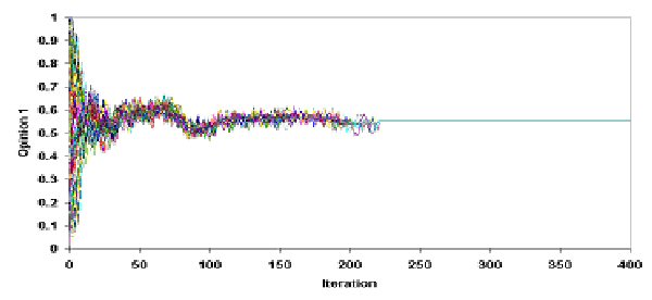
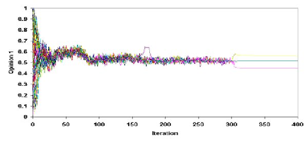
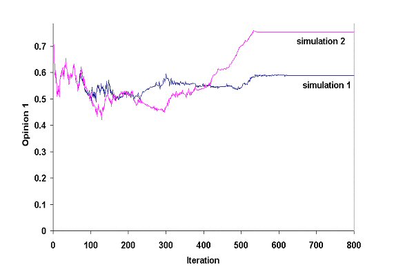
Figure 1. Opinion 1 of agent 1 in the two simulations (Ψ = 1.5 and ε = 0.1)

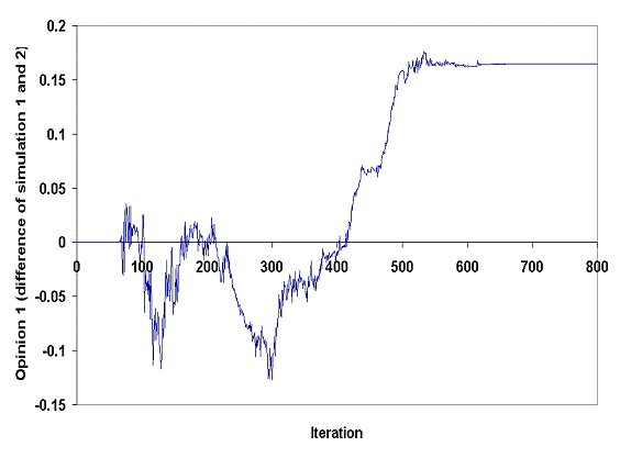
Figure 2. Differences of opinion 1 of agent (1) in simulations 1 and 2

4.4

This situation is typical for all agents. For example, agent (95) had exactly the same initial opinion 1 and 2 in both simulations but since we changed slightly the initial opinion 1 of Agent (1) the trajectories in the two simulations are quite different (see figure 3).

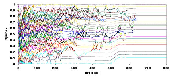
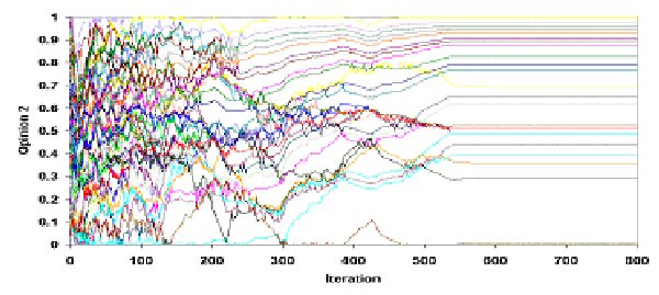
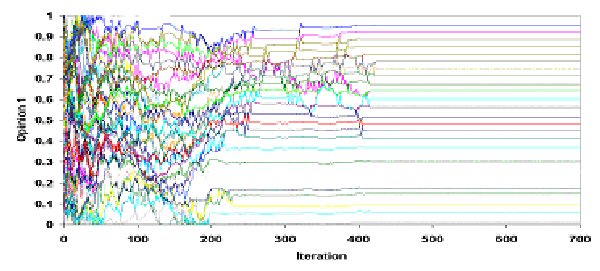
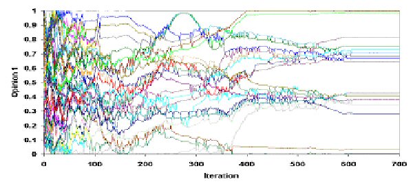
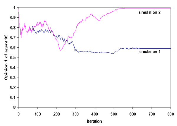
Figure 3. A minimal change on Agent (1) signifies a major change of Agent (95) -"Personal" history of Agent (95) according to two slightly different (in Agent (1), opinion 1) simulations of the MER model

4.5

We notice that the slightest perturbation in initial conditions causes a completely different outcome. Sensitivity to initial conditions is not limited to one agent who experienced the slight difference. As we know in such a system, each component of the system is highly interrelated with all others. This means that if we shift slightly one of them, all the others will be affected. For example, as presented on figure 3, the trajectories of agent (95) seems to be completely different according to our intervention in initial opinion 1 of agent (1). In table 5, we present both simulations (first column is the same with two columns of table 4) for all cases of Ψ = 1.5^[11].

4.6

The blue line is the trajectory of the opinion 1 of agent (1) in simulation 1 and the red line in simulation 2. We note that for about 70 iterations the difference of the opinions (see figure 2) remains tiny (of the rank of 10^-10) but after that it becomes significantly larger (of the same rank of the opinions themselves).

Ψ = 1.5 ε Simulation 1 Simulation 2 (e = 10-10 0.1 0.2 0.3

Table 5. System's dynamics with (simulation 2) or without (simulation 1) a small error (e = 10-10) in the initial opinion 1 of agent 1. Both agents' trajectories and final configurations are different due to sensitivity to initial conditions.

4.7

As we can see, the behaviour of the system differs significantly depending on a "slight" difference made in initial opinion of agent (1). In fact, we see that the observed dissimilarity is noteworthy: in both opinions, the dynamic of the systems as well as their final configurations are highly differentiated. This demonstration indicates clearly that in an "empirical" way our system seems to be unpredictable^[12].

Calculation of Lyapunov Exponents

4.8

In order to quantify the error propagation and examine whether MER model exhibits strong sensitivity to initial conditions and thus is unpredictable, we compute Local and Global Lyapunov Exponents^[13] for the values of Ψ and ε that we have studied our model up to now.

4.9

The ratio L that gives the error propagation for a specific iteration and an opinion profile is the Local Lyapunov Number, a measure of the stretching of the system, and its logarithm is Local Lyapunov Exponent (L > 1 if the error increases and L < 1 if it decreases). If we accumulate Local Lyapunov Exponents and take their average for a large number of iterations, we get (global) Lyapunov Exponent λ. Thus, Local Lyapunov Exponent is a local quantity averaged over a large number of iterations and gives (global) Lyapunov Exponent, a quantity that determines the average exponential rate of separation of two nearby initial conditions, or the average stretching of the space. For a more detailed mathematical description of Local and Global Lyapunov Exponents see Appendix C.

4.10

Therefore, a positive Lyapunov Exponent means that tiny errors increase on the average per iteration and nearby orbits move away, while a negative exponent means that nearby orbits are attracted (Peitgen et al 1992, p. 709-710). When the system is Lyapunov-positive, even slight perturbations in the system grow and predictability is lost. A positive Lyapunov Exponent signifies chaos (and thus unpredictability), a negative value implies a fixed point or a periodic cycle (Sprott 2003, p. 106) and a zero Lyapunov Exponent indicates a marginally or neutrally stable orbit (Kiel & Elliott 2000, p. 58).

4.11

We have calculated a running average of the Lyapunov Exponent (for Ψ = 0.5, 1 and 1.5 and ε = 0.1, 0.2 and 0.3) in order to ensure that the values settle to a unique number and test the reliability of the calculation^[14]. The results can be seen in table 6.

ε Lyapunov Exponent Information Entropy 0.1 0.2 0.3

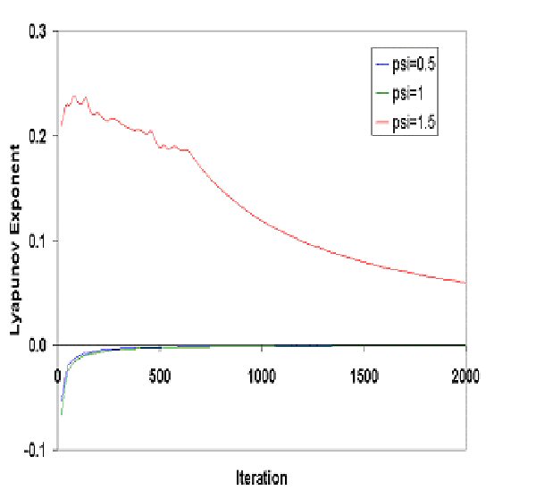
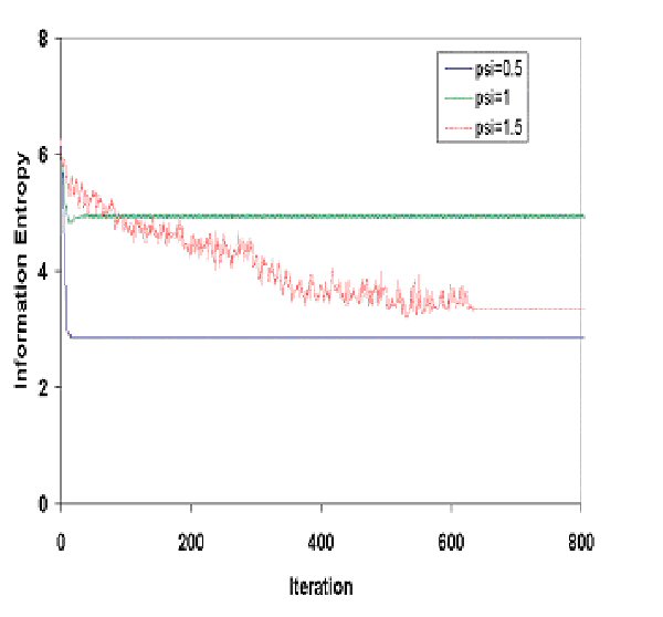
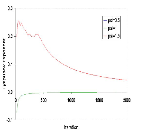
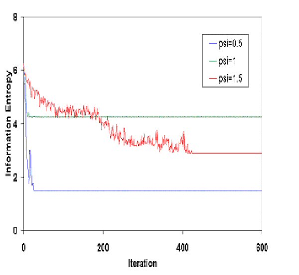
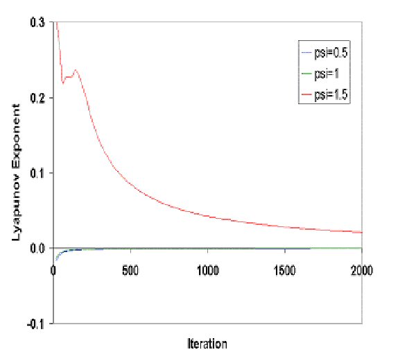
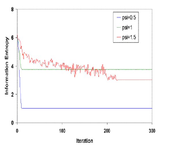
Table 6. Examining system's nonlinear characteristics: Lyapunov Exponents and Information Entropy

4.12

We notice that in all cases the running averages of Lyapunov exponents tend to zero. In other words, the (global) Lyapunov Exponent equals zero as expected, since all systems stabilize either in a fix point or in a periodic circle (final configurations can be seen in tables 2, 3 and 4^[15]). However, there is a difference in the way the averages converges to zero. For Ψ = 0.5 and Ψ = 1 the Local Exponents are negative for a small number of iterations. This is confirmed by the results presented in table 2, i.e. nearby trajectories of opinions come closer and tiny errors decrease or disappear. On the contrary, for Ψ = 1.5, Local Lyapunov Exponents are positive for a large number of iterations. This means that nearby trajectories of opinions move away and that the system is sensitive to initial conditions, at least for the first hundreds of iterations and it ends up in a final steady state (as can be seen clearly in table 4). This situation is referred to in the bibliography as final state sensitivity (Peitgen et al 1992, p. 757) or transient chaos (Sprott 2003, p. 173). This phenomenon may occur whenever there are several coexisting attractors. These attractors may be strange (Cambel 1993) or fixed points. In our case, every final state for a pair of parameter values for Ψ and ε is a fixed point in R²⁰⁰. The motion is apparently chaotic for a long time before eventually settling to a non-chaotic attractor. Obviously, the dimension of the attractors is low in all cases and equals the number of clusters for both opinions formed when the system stabilizes.

System's Information Entropy

4.13

According to Cambel (1993, p. 129-130) there is no best definition concerning the notion of entropy. The connecting link among the different forms of entropy is that, one way or another, they are indicative of deviation from equilibrium and chaotic behaviour. He suggests that anyone should use the best suited for his purposes and gives some possible definitions of entropy: "Entropy is the ability to reach equilibrium", or "an indication of transmitting information". In general, when Information Entropy increases the system becomes less uniform and more disorganized and when Information Entropy decreases the system becomes more uniform and more organized (Lugan 1993, p.18). In order to examine system's behaviour concerning its ability to self-organize, we have calculated Information Entropy or Shannon's Entropy for all iterations (for all Ψ and ε). For a more detailed account of the calculation of Information Entropy see Appendix D.

4.14

In table 6, we see that for Ψ = 0.5 and Ψ = 1 entropy decreases rapidly and smoothly (the system is self-organizing) and, after attaining its final state, it remains stable. For Ψ = 1.5, entropy decreases too, but it oscillates in a chaotic way (the system is self-organizing and self-disorganizing) until it reaches a flat line, which means that the system is stable. The results of information entropy's calculation demonstrate that our system for Ψ = 1.5 becomes highly unstable before it reaches its steady state.

Discussion: preliminary conclusions

5.1

MER model is based on simplicity, the simplicity of formalizing two psychosocial principles in terms of a methodological individualism^[16]. It has been clear that the setting of the parameters (ε and Ψ) plays a crucial role in the outcome. We have shown that if Ψ = 0.5, then the dynamics of the MER Model tends to be similar to these of the BC Model: the power towards an intra-individual equilibrium becomes trivial against the power for social equilibrium. For Ψ = 1, these two powers are of equal potency. Such a "balanced" setting leads the system to adopt the only kind of movement, which can be characterized both "harmonious" and "progressing": a periodic movement. For Ψ = 1.5, a strong drive for intra-individual equilibrium makes the system sensitive to initial conditions and thus unpredictable. This means that the system, in a surprising manner, exhibits transient chaos and that no formal typology of any kind can be applied in order to predict its emergent final state.

5.2

The experiments described above show that social action, theoretically supposed to seek the fulfillment of equilibria in combined form, can initiate unpredictability. Equilibrium is a motive whether it is social or individual: all agents search to attain synchronously such a state of stability (whether it is inter-individual, alias 'social', or intra-individual). However, because of this quest for two equilibria, unpredictability is generated: everything seems to be negotiated on the edge between social and individual. Each time that our agents "move" socially they destabilize their intra-consistency and, each time that they attain some kind of internal equilibrium, social influence comes to disturb them. Therefore, our system is complex, with emerging dynamics (Gilbert & Troitzsch 1999) and, although deterministic^[17], it is sensitive to initial conditions and unpredictable, i.e. chaotic.

5.3

With this work, we seek to demonstrate that models based on rigorous simplification are a promising method for understanding our real world of higher dimensions (Hegselmann & Flache 1998). Extremely broad theories of attitude's change were characteristic of earlier decades. In fact, anyone familiar with the history of attitude theory would quickly point out that the broadest theories were the theories of attitude change formulated in the 1950s and investigated empirically in the 1950s and 60s. Cognitive consistency theories were the major focus of interest during this era, with dissonance and balance theories attracting the major share of attention. Each of these theories attempted to encompass a wide range of attitudinal phenomena, through the use of a relatively small set of theoretical constructs. The popularity of these theories gradually declined, for a variety of reasons including undoubtedly a simple boredom with familiar ideas, which hastens shifts in zeitgeist^[18]. On the other hand, one of the main objections formulated against the "equilibrists", is that their models are much too purified and distant from the existing social reality, which hides much more surprises than they can ever predict. In other words, a world in equilibrium is a dull, stagnant and predictable world where no change should be expected and, finally, this should be a place almost inhuman to live within.

5.4

This demonstration tends to show that searching for error-free data collection techniques, is like "chasing chimeras": the only way out of this vicious circle is either to try to annihilate such an error or to accept that such a measurement is utopian. The sensitivity in initial conditions is a characteristic of the system itself and not a characteristic of the measurement tool applied. The initial position of the agents is extremely important in a precision, which makes the applied errors useless in psychological view: it is important however to say that such microscopic errors in opinion assessment can magnify themselves to a disproportional degree. Nevertheless, among many top scientists of this discipline there is always the "faith" that if we manage to control measurement error (and eliminate it!), then we will be capable of making exact predictions about human behavior and regain our place in the positivist elite (Aldridge 1999).

Appendix

A. Model of Multiple Equilibria Regulation (MER model)

A.1

We consider n = 100 agents, each of them assigned with two opinions at every iteration t. We denote x^k _t (i) ∈ [0,1] the opinion k of agent i at time t, t ∈ N, k = 1, 2, i ∈ {1, 2, … 100}. Let ε denote the bound of confidence and Ψ the intra-regulation factor. ε and Ψ are considered uniform for all agents. All opinions form two tables for each iteration and are called an opinion profile at iteration t. We suppose that an agent i arrives at a temporal revision tempx^k _t+1(i) of his opinion k by taking into account the opinions of all agents j that belong to the confidence set I(i, k, t) = {j ∈ N / 1 ≤ j ≤ 100, | x^k_t(i) – x^k_t(j) | ≤ ε }, t ∈ N, k = 1, 2, i ∈ {1, 2, … 100 }. In other words, the confidence set includes agents j that the difference in opinions x^k_t(i) – x^k_t(j) is in the confidence interval [- ε, ε].

A.2

The temporal opinion tempx^k_t+1(i) of agent i at iteration t+1 is the arithmetic mean of the opinions x^k_t(j) of all agents j that belong to the confidence set I(i, k, t), namely

where #I(i, k, t) denotes the number of elements of the set I(i, k, t).

A.3

We denote d_t(i) the maximum change of the absolute difference of the temporal opinions 1 and 2 with the previous opinions for agent i at iteration t, namely

where

A.4

If d_t(i) = |d¹_t(i)| then opinion 1 of agent i becomes the temporal one, i.e. x¹_t+1(i) = tempx¹_t+1(i), while opinion 2 moves to the opposite direction than opinion 1 was moved and we have x²_t+1(i) = tempx²_t+1(i) - Ψ · d¹_t(i), where Ψ is the intra-regulation factor.

A.5

The opposite happens if d_t(i) = |d²_t(i)|. This time opinion 2 of agent i becomes the temporal one, x²_t+1(i) = tempx²_t+1(i) while opinion 1 moves to the opposite direction than opinion 2 was moved and we have x¹_t+1(i) = tempx¹_t+1(i) - Ψ · d²_t(i). The same procedure takes place for all agents synchronously (updating is simultaneous).

B. Pseudocode of the actions performed at each time step (iteration).

A.6

ε	Bound of confidence
Ψ	Intra-regulation factor
Opinion (i, p)	Opinion p, p ∈ {1, 2} of agent i at the previous iteration.
TemporaryOpinion (i, p)	The mean of the Opinions of agents j that their Opinion differ from agent i less than the Bound of Confidence ε.
NewOpinion (i, p)	Opinion p of agent i at the next iteration.
Abs	Absolute Value

For all opinions p
		For all agents i 
			Sum=0: Counter=0
			For all agents j
				Distance (i, j, p) = Abs (Opinion (i, p) – Opinion (j, p))
				If Distance (i, j, p) <= ε Then
    				Counter = Counter + 1
    				Sum = Sum + Opinion (j, p)
				End If
			TemporaryOpinion (i, p) = Sum / Counter
For all agents i 
		For all opinions p
			Change (p)= TemporaryOpinion (i, p) – Opinion (i, p) 
		Max=Maximum { Abs (Change (1)),  Abs (Change (2)) }
		If Max= Abs (Change (1)) Then
			NewOpinion (i, 2) = TemporaryOpinion (i, 2) - Ψ * Max
		If Max= Abs (Change (2)) Then
			NewOpinion (i, 1) = TemporaryOpinion (i, 1) - Ψ * Max
For all opinions p
		For all agents i 
			Rescale NewOpinion (i, p) into [0,1]
Calculate Information Entropy
Calculate Lyapunov Exponent

C. Lyapunov Exponents

A.7

The main idea for the calculation of the Lyapunov Exponent is this: By an opinion profile x we mean a vector with 200 components, each one into the interval [0,1], the first 100 denoting the opinions 1 of the 100 agents and the rest the opinions 2 (x ∈ R²⁰⁰). We consider two initial profiles, x₁ and another one x₂ that carries an error e₀ = 10 ^-10 in connection with x₁ (i.e. the Euclidian distance of x₁ and x₂ in R²⁰⁰ equals e₀). We iterate both x₁ and x₂ separately and we get y₁ and y₂ respectively, with their Euclidian distance being e₁. The ratio e₁/ e₀ = L quantifies how the error is amplified (the error increases if L > 1 and decreases if L < 1). L is called Local Lyapunov Number (also relative error per iteration or error amplification factor) and its logarithm Local Lyapunov Exponent. We record this ratio. In order to continue the procedure, we keep opinion profile y₁ and move opinion y₂ so that it has a distance of e₀ with y₁, without changing the direction of y₂ - y₁ ∈ R²⁰⁰. We iterate opinions y₁ and y₂, we accumulate Local Lyapunov Exponents and take their average for a large number of iterations. This is the (global) Lyapunov Exponent λ. Thus, Local Lyapunov Exponent is a local quantity averaged over a large number of iterations and gives the (global) Lyapunov Exponent.

A.8

For a more detailed explanation about Lyapunov Exponents see Peitgen et al (1992), Sprott (2003) or Alligood et al (1996) and for a program in Basic for the calculation of the Lyapunov Exponent see Sprott (1998).

D. Computation of the information entropy of the system.

A.9

We calculate the Information Entropy of the simulation for each iteration using the formula (Peitgen et al 1992)

A.10

The computation goes like this: We divide the interval [0,1] into 100 intervals of equal length B₁ = [0, 0.01], B₂=[0.01, 0.02] and in general B_k = [(k-1)/100, k/100], k=1,2 … 100. For every interval B_k we compute the probability P(B_k) of an agent's opinion to belong into the interval B_k by dividing the number of the agents that their opinion belongs to B_k with the total number of agents. We sum up for the 100 intervals B_k the product of the probability P(B_k) times the logarithm with base 2 of P(B_k) and we obtain Information Entropy with the opposite sign.

Acknowledgements

We would like to thank Professor Tassos Bountis, Department of Mathematics, University of Patras for stimulating discussions and helpful suggestions.

Notes

¹ As referred by Hegselmann & Krause (2002) this model has been developed by Krause (1997, 2000); see also Beckmann (1997), Dittmer (2000, 2001), Deffuant et al. (2001), Deffuant et al. (2002), and Ben-Naim et al. (2003).

² This conflict is defined as a psycho-logical concept and not on a pure logical basis.

³ These inter-relations among cognitive elements (CE) can be of three kinds: consonant, dissonant and irrelevant (Festinger 1957).

⁴ In our paradigm, opinions have a sentence-like form: they can be defined as cognitive elements (CE) of the same cognitive space: i.e. if CE A goes up then CE B must go down or vice-versa.

⁵ Maybe the word "conforming" is more suitable in our case (Sherif 1936; Asch 1951, 1956).

⁶ Of course, as for social equilibrium, a state of achieved "Intra-individual" equilibrium is purely theoretical (see Introduction on Intra-individual equilibrium). Therefore, to be more exact, a person rather "tries" to attain the equilibrium than "maintaining" an already achieved equilibrium.

⁷ Just like rhinoceros, one is considered "myopic" in static values but accurate in changes. A rhinoceros is very deficient in seeing static things but he distinguishes motion easily.

⁸ For the moment, we consider that values above 2 are rather "unrealistic". This means that adding or subtracting the double of the difference found in one opinion to the other can already be characterised as "over-reaction".

⁹ This procedure is like every time some opinion escapes the interval [0,1] we "photocopy" the opinions by reducing their size proportionally and so we put them into [0,1] again. We have tested for a large number of parameter values that the dynamical behavior of the system is unaltered and thus we obtain similar configurations.

¹⁰ Given the expected measurement error produced in every data collection technique concerning social phenomena, the magnitude of "error" can be extremely high (or even "gross") in terms of exact sciences' mathematical analysis. This means that an error of the order 10^-10 is simply senseless in socio-psychological research and one considers that social sciences' measurement cannot be "exact", so these sciences could never enter the "exact sciences club".

¹¹ We do not present simulation 2 for Ψ = 0.5 and Ψ = 1, since in these cases the initial error becomes even smaller or disappears. The system gives exactly the same picture for simulation 2, as we can see for simulation 1 in table 2 and apparently does not exhibit sensitivity to initial conditions.

¹² Sensitivity, however, does not automatically lead to unpredictability. Indeed, there are sensitive systems that are predictable, e.g. the linear transformations x_n+1 = c · x _n, c ∈ R, n ∈ N^*. An initial error is magnified after we iterate, but the error remains significantly smaller than x_n (Peitgen et al 1992, pg.512). In a chaotic system, given the slightest deviation in initial conditions, after a certain number of iterations, it will become as large as the true signal itself. In other words, the error will be of the same order of magnitude as the correct values.

¹³ For every pair of values for Ψ and ε the system has 200 Lyapunov Exponents since it is defined in R²⁰⁰. In all cases, we compute only the Larger Lyapunov Exponent, which is the best indication for the predictability or unpredictability of the system.

¹⁴ We have also tested that the values of the Lyapunov Exponents calculated above are independent of the magnitude of error (when error tends to zero) and independent of different initial conditions.

¹⁵"Final configuration" stands for the system position beyond which there is no further change of values.

¹⁶ The simplest way of defining methodological individualism is the thesis in which every proposition about a group is, implicitly or explicitly, formulated in terms of behavior or interaction of the individuals constituting the group (Schumpeter 1908).

¹⁷ Our model does not include any stochastic process; therefore, the trajectories of our agents are predetermined by means of interaction's algorithms.

¹⁸"Zeitgeist" means a trend of a culture and taste characteristic of an era.

References

ALDRIDGE, A. (1999). Prediction in Sociology: Prospects for a Devalued Activity. Sociological Research Online, vol.4, No 3.

ALLIGOOD, K. T., Sauer, T. D. & Yorke, J. A. (2000). Chaos, an Introduction to Dynamical Systems. New York: Springer-Verlag.

ASCH, S. E. (1951). Effects of Group Pressure upon the Modification and Distortion of Judgement. In H. Guetzkow (Ed.). Group, Leadership and Men. Pittsburgh, PA: Carnegie Press. (p. 177-190)

ASCH, S. E. (1956). Studies of Independence and Conformity: 1. A Minority of one Against a Unanimous Majority. Psychological Monographs. 70 (9, No 416)

AXELROD, R. (1997). Advancing the Art of Simulation in the Social Sciences. Complexity, Vol. 3, No 2, p. 16-22.

BECKMANN, T. (1997). Starke und schwache Ergodizität in nichtlinearen Konsensmodellen. Diploma thesis Universität Bremen.

BEN-NAIM, E. Krapivsky, P. & Redner, S. (2003). Bifurcations and Patterns in Compromise Processes. Physica D 183 190.

BILLIG, M. (1991). Ideology and Opinions. London: Sage Pbns.

BUCKLEY, W. (1967). Sociology and Modern Systems Theory. Englewood Cliffs: Prentice-Hall

CAMBEL, A. B. (1993). Applied Chaos Theory: A paradigm for Complexity. Academic Press, Inc.: San Diego, USA.

CASTI, J. L. (1994). Complexification: Explaining a Paradoxical World Through the Science of Surprise. London: Abacus.

DEFFUANT, G. Neau, D. Amblard, F. and Weisbuch, G. (2001). Mixing beliefs among interacting agents. Advances in Complex Systems, 3, 87-98.

DEFFUANT, G. Amblard, F. Gérard Weisbuch, G. & Faure, T. (2002). How can extremism prevail? A study based on the relative agreement interaction model. Journal of Artificial Societies and Social Simulation vol. 5, no. 4

https://www.jasss.org/5/4/1.html

DITTMER, J. C. (2000). Diskrete Michtlineare Modelle der Konsensbildung. Diploma thesis Universität Bremen.

DITTMER, J. C. (2001). Consensus Formation Under Bounded Confidence. Nonlinear Analysis, 47(7), p. 4615-4621.

FESTINGER, L. (1957). A Theory of Cognitive Dissonance. Evanston, IL.: Row, Peterson.

FISKE, D. W. & Shweder R. A. (1986). Metatheory in Social Science. Chicago and London: The University of Chicago Press.

FLAMENT, C. (1981). L' Analyse de Similitude: Une Technique pour les Recherches sur les Représentations Sociales, Cahiers de Psychologie Cognitive, 4, p. 357-396.

GERGEN, K. J. (1973). Social Psychology as History. Journal of Personality and Social Psychlogy. 26: 309-20.

GILBERT, N. & Troitzsch, K. G. (1999). Simulation for the Social Scientist. London: Open University Press.

HEIDER, F. (1946). Attitudes and Cognitive Organization. Journal of Psychology, 21, 107-112.

HALFPENNY, P. (1997). Situating Simulation in Sociology. Sociological Research Online, vol. 2, No 3.

HEGSELMANN, R. & Flache, A. (1998). Understanding Complex Social Dynamics: A Plea For Cellular Automata Based Modelling. Journal of Artificial Societies and Social Simulation, vol. 1, no 3. https://www.jasss.org/1/3/1.html

HEGSELMANN, R. & Krause, U. (2002). Opinion Dynamics and Bounded Confidence Models, Analysis and Simulation. Journal of Artificial Societies and Social Simulation, vol. 5, no 3. https://www.jasss.org/5/3/2.html

KIEL, L. D. & Elliott, E. (1997/2000). Chaos Theory in the Social Sciences. USA: The University of Michigan Press.

KRAUSE. U, (1997). Soziale Dynamiken mit vielen Interakteuren. Eine Problemskizze. In Krause, U. and Stockler, M. (Eds.) Modellierung und Simualation von Dynamiken mit vielen interagierenden Akteuren. Universitat Bremen, p. 37-51.

KRAUSE, U. (2000). A Discrete Non-linear and Non-autonomous Model of Consensus Formation. In Elaydi, S., Ladas, G., Popenda, J. and Rakowski, J. (Eds.). Communications in Difference Equations. Amsterdam: Gordon and Breach Publ. p. 227-236.

LEWIN, K. (1936). Elements of a Topological Psychology. New York: McGraw-Hill.

LUGAN, J-C. (1993). La Systémique Sociale. Paris: P.U.F. (Q-S-J)

PARETO, V. (1916/1935). Mind and Society, USA: Kensington Publishing Co.

PARSONS, T. (1977). Social Systems and the Evolution of Action Theory. New York: The free Press

PEITGEN, H-O. Jurgens, H. & Saupe, D. (1992). Chaos and Fractals, New Frontiers of Science. New York: Springer-Verlag.

PERELMAN, C. (1979). The new Rhetoric and the Humanities. Dordrecht: D. Reidel.

SCHUMPETER, J. (1908). On the Concept of Social Value. Quarterly Journal of economics, p. 213-232.

SHERIF, M. (1936). The Psychology of Social Norms. New York: Harper and Brothers.

SOROKIN, P.A. (1927). Social Mobility. New York: Harper.

SPROTT, J.C. (1998). Numerical Calculation of Largest Lyapunov Exponent. http://sprott.physics.wisc.edu/chaos/lyapexp.htm

SPROTT, J.C. (2003). Chaos and Time-Series Analysis. Oxford University Press: Oxford.

Return to Contents of this issue

© Copyright Journal of Artificial Societies and Social Simulation, [2004]