© Copyright JASSS

  JASSS logo ----

Matthias Scheutz and Paul Schermerhorn (2004)

The Role of Signaling Action Tendencies in Conflict Resolution

Journal of Artificial Societies and Social Simulation vol. 7, no. 1
<https://www.jasss.org/7/1/4.html>

To cite articles published in the Journal of Artificial Societies and Social Simulation, please reference the above information and include paragraph numbers if necessary

Received: 08-Jun-2003      Accepted: 14-Sep-2004      Published: 31-Jan-2004


* Abstract

We investigate various strategies for stopping games embedded in the larger context of an artificial life simulation, where agents compete for food in order to survive and have offspring. In particular, we examine the utility of letting agents display their action tendencies (e.g., "continue to play" vs. "quitting the game" at any given point in the game), which agents can take into account when making their decisions. We set up a formal framework for analyzing these "embedded stopping games" and present results from several simulation studies with different kinds of agents. Our results indicate that while making use of action tendency cues is generally beneficial, there are situations in which agents using stochastic decision mechanisms perform better than agents whose decisions are completely determined by their own and their opponents' displayed tendencies, particularly when competing with agents who lie about their action tendencies.

Keywords:
Conflict Resolution, Stopping Games, Signaling

* Introduction

1.1
Stopping games (e.g., Shmaya and Solan 2002, Solan and Vieille 2002, Touzi and Vieille 2002, and Solan and Vieille 2001) are ones in which two agents engage in repeated interactions until one agent decides to quit, at which point the payoff for both agents is determined. They appear in many social contexts. For example, bidding in an auction can be viewed as a stopping game in which the winner receives the prize when no other bidder is willing to raise her bid. Similarly, when animals fight for food, the contest ends and the payoff is given when one participant does not continue. In the latter case, especially, there are aspects of the context of the game, which are typically ignored in formal game-theoretic analyses of stopping games. Perhaps the most important one is the fact that contestants are continuously paying a price for playing the game. In a poker game, for example, this price is the cost of bidding in each round, while in the hiring of employees it is the company's investment during the selection and interviewing process (the reviewing of resumes, the on-site interview, etc.). In a biological setting, the cost is determined in terms of the energy that animals expend during their fights, which creates the interesting possibility that one (or both) of the players will run out of resources and be removed from the game (i.e., die). Normal analyses of stopping games are conducted in isolation of such constraints imposed by the contexts in which the games are embedded. We will focus on a biological setting in this paper and argue that such contexts can critically matter to the selection of good strategies.

1.2
When animals fight for resources (food, mates, territory, etc.), the contests typically involve displays of aggression or prowess (e.g., Adamo and Hanlon 1996, Decoursy and Jenssen 1994, and Hofmann and Schildberger 2001). These demonstrations of strength can be construed as the display of the probability with which an animal will continue to fight (if put in a contest): roughly speaking, the stronger the display (e.g., of aggression), the higher the likelihood that the animal will keep fighting after a given time. Several questions arise: (1) is displaying this information beneficial, (2) what strategy should animals play, (3) is there an optimal strategy, and (4) is cheating (i.e., displaying wrong action tendencies) beneficial (at the individual and/or the group level)?

1.3
We consider a particular kind of embedded stopping game: the competition for food in the larger context of foraging for food. In this embedded game, agents need to find food in order to survive and be able to procreate. Each agent has an internal energy store, from which energy is subtracted for movements, fighting, and even just existing. In other words, there is a cost associated with each action which is measured in terms of energy, and ingesting food is the only way to replenish the internal energy store. During each agent's search for food, there may be occasions in which two or more agents are trying to obtain the same food source. These encounters then lead to the embedded stopping games, where agents can decide to quit and leave the food for the other agent(s), or to fight for food. Costs (e.g., for fighting) are assessed at every step of the game. When participants run out of resources, they are removed from the (larger) game, and hence cannot have offspring. In the evolutionary context, this means that their genes are not passed on.

* Stopping Games with Signaling

2.1
In stopping games players typically do not signal their probabilities to quit to other agents. In fact, in games like poker players attempt their best to hide a their action tendencies (i.e., to avoid signaling them overtly or covertly). Consequently, in such games players generally do not have the possibility to take the propensities of other players into account and, hence, have to develop a strategy that is entirely based on their own propensities. In a biological setting, however, animals do indicate to other animals the extent to which they are willing to fight (regardless of whether this indication is always true or sometimes false, or whether they actually "know" what they are going to do). The mere fact that many species do display their action tendencies suggests that it might be advantageous as a mechanism for resolving social conflict.

2.2
The stopping game with signaling that we examine here is one in which agents engage in conflicts over resources and continue to fight until one participant (or both) chooses to break off the conflict (i.e., retreats) or runs out of resources and is removed from the simulation (i.e., dies). Retreating agents incur a cost of stopping (CS) that represents the energy consumed fleeing from their opponents. Agents that choose to continue incur an analogous cost of fighting (CC). Agents that win an encounter (i.e., that are the last remaining agent in the encounter) acquire a benefit (BC) representing the value of whatever resources were being contested. Retreating agents also have some probability of acquiring resources elsewhere, which is the benefit of stopping (BS). Each instance of this stopping game with signaling is embedded in another game that is simply the competition between agents to acquire resources and, ultimately, reproduce. Embedding the game in this overall context rewards efficient conflict resolution mechanisms that end conflicts as quickly as possible by increasing agents' chances of surviving and reproducing and punishes inefficient mechanisms by increasing the possibility that they will die.

2.3
In this game, continuing is expensive when one's opponent also chooses to continue, because neither will receive any payoff, while both will pay the cost CC. Similarly, choosing to stop when one's opponent also chooses to stop leads to neither agent receiving the reward BC. The best outcome overall is a mixed outcome in which one agent decides to continue while the other decides to stop. In that case, each contestant will incur some cost (CC or CS), but will also have the opportunity to reap some benefit (BC or BS).

2.4
The payoff matrix for an n + 1 stage game is


StopContinue

Stop(BS+CS+n×CC, BS+CS+n×CC)(BS+CS+n×CC, BC+CC+n×CC)
Continue(BC+CC+n×CC, BS+CS+n×CC)
N/A

where

CC, CS < 0 < BS < BC. (1)

2.5
This table makes clear the benefit of short encounters for both agents; long encounters accrue large costs while not increasing the benefit gained at the end of the game.

2.6
As mentioned before, we allow agents to signal their action tendencies (i.e., a probability to continue the game). Typically, the signal an agent presents will be its probability of quitting as determined by the strategy it is playing. However, agents are not constrained to telling the "truth" about their action tendencies, but may signal whatever they like (e.g., they could attempt to deceive other agents who rely on the truthfulness of the display), although for some signaling mechanisms (e.g., perspiration or flushed skin tone) it may be impossible for agents to change their signal (e.g., because the signaling mechanism is hard-wired).

* The Utility of Signaling

3.1
The game described above is used to explore the benefits of signaling action tendencies to other agents who, in turn, may take these signals into account in their decision to continue playing in an embedded stopping game. When two agents, A and B, play a game, it is best for A to continue when it believes that B is going to stop, and to stop when it believes that B is going to continue. It is in A's best interest, then, for B to signal its tendency for conflicts so that A can better predict B's future actions. However, it is also in B's best interest (in many cases) to provide such signals, because they may convince A that continuing is less appealing, making it more likely that B will obtain BC. There are cases, of course, in which B's signal will make the prospect of continuing more appealing to A (i.e., when B's tendency is weaker than A's), thereby decreasing the probability that B will obtain BC, but even in those cases signaling will also decrease the probability of long games, which is beneficial to all contestants.

3.2
In investigating the benefits of signaling, i.e., whether the presence of cues and the ability to use them are beneficial to agents, we should, however, not make any assumptions about an agent's willingness to signal or truthfulness in signaling. Furthermore, we should not make assumptions about agents taking signals into account (some agents may either not have the ability to signal or may not care about other agents' signals). Hence, different mixed groups of strategies need to be studied to determine whether signaling is beneficial, in particular if an evolutionary case about the likelihood of the evolution of signaling systems in such embedded games is to be made. In the following, we define a simple formalism, which allows us to study mixed groups of strategies.

* A Formalism to Express the Degrees of Sociality of Agents

4.1
There are several possible ways to approach a formalism for taking other agents' action tendencies into account that can vary in influence from weak (agents that take only their own action tendencies into account) to strong (agents that take their opponents' tendencies into account to such a degree that they will only choose to continue if the opponent is less likely to do so). For example, one could keep track of the degree to which agents "trust" the display of other agents. Depending on that trust factor, agents could then decide what to do at any given stage in the game. Alternatively, one could determine what to do as a function of one's own display and the other's display. The mechanism described below works by iteratively applying a comparison procedure to the displayed tendencies of both agents m times, where m indicates the degree to which the agent takes others' tendencies into account. This has the advantage that we can define an infinite class of agents, call them "m-social," that cover the whole range from ignoring another agent's display to taking it into account maximally. With this in mind, we refer to agents that use only their own action tendencies to decide their actions as "0-social" agents, while we refer to those that make maximal use of cues from other agents as "∞-social" agents. Between these two extremes are agents that make use of opponents' signals to varying degrees m (i.e., referred to as "m-social" agents).

4.2
It is worth mentioning that an m-social agent can also be interpreted as "trusting" the veracity of another agent's display to a certain degree determined by m: the higher m, the greater the trust, which culminates in "∞-social" agents who trust the other agent's display so much that they reach a final decision immediately. Conversely, the "0-social" agents do not trust other agents, which is apparent from the fact that they do not take other agents' displays into account at all.

4.3
Given that we want to construe an agent's action tendency as "related" to its probability to continue a game, action tendencies need to be mapped into [0,1] with DS representing an agent's own action tendency and DO representing its opponent's perceived action tendency. Agents can then interpret opponents' action tendencies as the probabilities they will continue. An agent's own probability of continuing is generally also based on its own action tendency.

4.4
The degree to which an agent's action tendency to continue is mediated by its opponent's perceived action tendency is determined by the function g:[0,1]×[0,1]→[0,1], which can be defined in terms of the three functions g+(DS, DO), g0(DS, DO), and g(DS, DO), producing PC, the probability that the agent will continue, as follows:

PC = g+(DS, DO)if DS > DO
= g(DS, DO)if DS < DO
= g0(DS, DO)if DS = DO
(2)

4.5
When DS is greater than DO, g+(DS, DO) is applied to DS to produce the probability that the agent will decide to continue (PC). The function g+(DS, DO) must be defined such that DS,DO (DS > DO → DS < g+(DS, DO) ≤ 1). That is, when the agent's action tendency to continue is greater than its opponent's, the agent's action tendency is increased, making it more likely to decide to continue. However, the most it can be increased is the difference between the original value and 1 (i.e., it can never be increased above 1). When DS < DO, g(DS, DO) is applied to DS to produce PC. The function g(DS, DO) must be defined such that DS,DO (DS < DO → 0 ≤ g(DS, DO) < DS). So when the agent's action tendency to continue is less than its opponent's, the agent's action tendency is decreased, making it less likely to continue. However, the most it can be decreased is the difference between 0 and the original value (i.e., it can never be reduced below zero). Finally, when the action tendencies are equal, then g0(DS, DO) is used, which typically will be DS = DO.

4.6
Using the above functions, we can now formally define the notion of "m-social agent", where the associated value m represents the degree to which the agent takes its opponent's action tendency into account when making its decision whether to continue. Note that m can be thought of as the agent's degree of "sociality" (in the context of this game). We use m to define a function h, which consists of the three functions h+(DS,DO)m, h0(DS,DO)m h(DS,DO)m to determine the number of times g(DS,DO) is recursively applied to DS (for g∈{g+,g0,g}).

h+(DS,DO)0 = DS
h+(DS,DO)m + 1 = g+(h+(DS,DO)m,DO)
h0(DS,DO)0 = DS
h0(DS,DO)m + 1 = g0(h0(DS,DO)m,DO)
h(DS,DO)0 = DS
h(DS,DO)m + 1 = g(h(DS,DO)m,DO)
(3)

4.7
While any function g that is monotonically increasing for DS > DO and monotonically decreasing for DS < DO can be used, we would like a function g* such that h* defined in terms of g* actually converges to 1 from any DS >DO (for a fixed DO) if m goes to infinity (and similarly for the 0 in case of DS <DO). We chose the following functions for g*:

g*+(DS, DO) = DS + ((1 - DS) / DS) × (DS − DO)if DS > DO
g*0(DS, DO) = DSif DS= DO
g*(DS, DO) = DS − (DS / DO) × (DO − DS)if DS < DO
(4)

4.8
These equations map the difference in D values for the two agents into the space available by scaling the difference by the amount between DS and 1 (or 0). The result is an increase or decrease in an agent's probability of fighting depending on whether the agent's action tendency value DS is higher than its opponent's or not. In this way, agents are able to make more "informed" decisions in conflicts, and can reduce costly continue-continue and stop-stop outcomes. Figure 1 shows the performance of g*+ and g* for various combinations of DS and DO (where DS + DO = 1). They converge within a few iterations. Furthermore, it follows directly from this definition that 0-social agents do not consider their opponent at all; their decision to continue is based solely on their own action tendencies. Finally, it follows that ∞-agents always continue when their opponents' action tendencies are less than their own and always stop otherwise.

Fig 1
Figure 1. Decision Mechanism Performance. Lines are paired by color, each pair representing a contest in which the two agents' D-values sum to 1. The probabilities of continuing at 0 iterations are just the original D-values; thereafter the probabilities diverge from one another (except in the (0.5,0.5) case) according to the rule described above

4.9
Assuming a Gaussian distribution of action tendencies and based on the game matrix for embedded games, we predict that m-agents for m > 0 will outperform 0-agents (i.e., the "asocial" ones) and, hence, that taking the action tendencies of other agents into account is beneficial. In particular, ∞-agents should to do best if put in environments without liars (i.e., agents that do not truthfully signal their action tendencies), since the combined payoff for both agents is maximal in a one round game. Furthermore, the strategy played by ∞-agents prevents them from playing multiple games for the same food item among each other, whereas other m-agents might end up fighting for the same resource several times, namely when both agents decide to retreat at the same time, but then end up coming back again. For sufficiently large m we expect that m-agents will show the same performance as ∞-agents. For environments with liars, however, we predict that being social can be problematic depending on the degree to which agents lie about their action tendencies. In particular, we expect that the more social agents are, the more they can be exploited by liars, especially if they lie all the time, displaying 1 as their action tendency. In such environments, ∞-agents should to do worse than m-agents for any m.

* Experimental Setup

5.1
In order to determine the effect of allowing agents to use opponents' tendency cues in stopping games, we implemented agents with that ability in the artificial life environment SimWorld (Scheutz and Schermerhorn 2002). In this environment, agents forage for food to meet their energy requirements, and procreate when they have obtained sufficient energy reserves (they use a "need-based" foraging strategy as defined in Scheutz 2001). When agents come into close proximity, they can choose either to stay (potentially acquiring any resources in the area) or to retreat (passing up on the resources, but also not paying the cost of staying). Agents display their action tendencies for conflict situations, and are able to read these cues to get information about what their opponents are likely to do (except when facing cheaters; see below). Agents are assigned action tendencies at birth in a Gaussian distribution between 0 (never continue) to 1 (always continue) to allow us to study diverse populations.

5.2
The simulation environment (see Figure 2) is an unbounded, continuous two-dimensional plane, with food sources generated at random locations within a 1440 by 1440 area with a probability of 0.5 (i.e., there is a 0.5 probability each turn that one food source will be generated). Agents are free to leave the region in which food is generated, but must return to eat in order to survive.

Fig 2
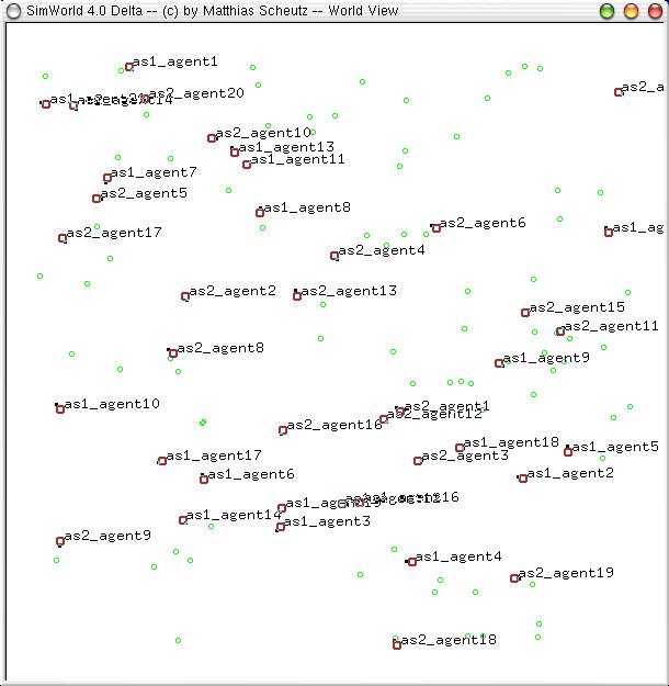
Figure 2. The SimWorld artificial life environment (graphical mode); small green circles represent food sources and red circles represent agents, with black tics indicating agents' headings. Here, 0-social agents (labeled "as1_agent" followed by their ID number) are competing against m-social agents (labeled "as2_agent" followed by their ID number)

5.3
The following pseudo-code shows the main loop of the simulation, which is called for each update cycle:


;;; the loop to update one simulation cycle 
foreach cycle do
    generate new food resources
    foreach entity in allentities do
        percepts(entity) := run_sensors(entity, allentities)
    endforeach
    foreach entity in allentities do
	actions(entity) := run_rulesystem(entity, percepts(entity)) 
    endforeach
    foreach entity in allentities do
	perform actions(entity)
    endforeach
    remove dead agents, update agents' body representations, update counters
    perform statistics
endforeach

5.4
Of particular interest is the function run_rulesystem, which updates the state of each agent. In particular, it detects conflicts and determines whether the agent should fight or retreat:


;;; select actions based on percepts
function run_rulesystem(entity, percepts) returns action;
    generate a combined force vector for the percepts
    opponent := detect_opponent(percepts)
    if exists(opponent) then
	P := entity.tendency
	if infinite-social(agent) then
	    if entity.tendency > opponent.display then
		P := 1
	    else
		P := 0
	    endif
	else
	    for i from 1 to entity.iterations do
		if P > opponent.display then
		    P := P + ((1 - P) / P) * (P - opponent.display)
		else
		    P := P - (P / opponent.display) * (opponent.display - P)
		endif
	    endfor
	endif
	if P ≥ random(1.0) then
	    action := retreat (i.e., generate force away from opponent)
	else 
	    action := fight (i.e., set force to 0)
	endif
    else
        action := move as determined by the force vector    
    endif
endfunction

5.5
The run_rulesystem procedure is called for each entity every round. Agents compute force vectors from other agents and food resources. These force vectors are weighted and combined to generate a force vector indicating the direction the agent wishes to move (e.g., toward food and away from obstacles) in the following way:

motion_vector = 20 * ( ∑VF (1 / |VF|2 * VF)) - 20 * ( ∑VS (1 / |VS|2 * VS)) - 5 * ( ∑VO (1 / |VO|2 * VO)) . (5)

5.6
This sums the vectors (VF) from the agent to each food item, scaled by 1 / |VF|2, and multiplies the result by the gain value of 20. That is added to similarly summed force vectors for agents of the same kind as the current agent (VS) and agents of other kinds (VO), multiplied by gains of -20 and -5, respectively, to obtain the default motion vector for the agent. When there is another agent within conflict range, the agent must decide whether to fight or retreat. This is accomplished with an implementation of the formulas given above. ∞-social agents are special cases whose probabilities are determined directly. Otherwise, the iterated formula is applied. Note that for 0-social agents (i.e., agents whose "iterations" value is 0), P remains unchanged.

5.7
Experiments run for 10,000 cycles, and start with 20 instances of each agent kind specified. The measure of performance used is the number of surviving agents, averaged over 80 experimental runs with different random initial conditions.

5.8
Agents are assessed a cost of 50 units of energy (CC) when they decide to continue a game. This cost may be assessed many times, depending on how long the game lasts. The utility of winning averaged between 275 and 345 units, depending on the experiment (see Figure 3). This value represents the value of food acquired (BC), if any, between the time the current game ended and the next game started; it does not include the cost CC assessed at each turn of the game. The net benefit of losing averaged between 120 and 165 units of energy, again depending on the experiment (see Figure 4). This value represents both the value of any food acquired after retreating from the encounter (BS) between the time the game ended and the next game began. At the time of retreat, the agent is assessed the cost of retreating (CS) of (on average) 245 units. This represents the cost of running at an increased speed for several cycles. Note that this cost is spread out over 10 cycles, on average, whereas the cost of continuing is assessed each turn.

Fig 3
Figure 3. Utility of Winning

Fig 4
Figure 4. Utility of Losing

5.9
In Figures 3 and 4, the utilities tend to decrease as m increases, especially in the case of the 0-social vs. m-social experiments. Since the utility of either winning or losing is just the probability of finding food to consume times the value of that food, and the value of food is fixed, the probability of finding food in environments with higher values of m must be lower. This is because, as the value of m increases, the average length of the games becomes shorter. Therefore, more agents are foraging rather than engaging in conflicts, and the amount of food present in the environment goes down. The 0-social vs. m-social environments have the most dramatic decrease in the length of conflicts because the number of agents more likely to enter into long conflicts decreases at the same time the number of agents less likely to enter into long conflicts increases (see Figure 5 below). In the other cases, the ratios do not change as dramatically (see Figures 6, 7, and 8 below).

5.10
The performance of each agent type in homogeneous environments (i.e., when agents are competing only with agents of their own kind) provides a baseline against which later results can be compared. These were very similar for all types, ranging between 51.64 (for 0-social agents) and 55.66 (for ∞-social agents). Each agent type's performance is very similar to its neighbors' (i.e., (m - 1)-social and (m + 1)-social agents), although the difference between 0-social and ∞-social agent performance is statistically significant.

* Simulation Results

6.1
The first set of experiments compares the performance of 0-social agents with m-social agents for m > 0. Figure 5 shows the results of these tests. (Note that for Figures 5 through 8, confidence intervals are given for α = 0.05.) 1-social agents already outperform the 0-social agents. As the value of m increases, m-social agents perform progressively better relative to 0-social agents. The final data point in Figure 5 (labeled as "∞") presents the results from environments in which 0-social agents compete with ∞-social agents. ∞-social agents essentially compare the displayed action tendency of their opponents with their own, and continue if their tendency is higher than that of their opponent. Otherwise, they stop. It is interesting to note that 10-social agents are already performing very similarly to ∞-social agents against 0-social agents.

Fig 5
Figure 5. 0-social vs. m-social

6.2
The next set of experiments compares the performance of m-social agents for m < ∞ with ∞-social agents. Figure 6 presents the results of these experiments. Here, again, we see that within ten iterations, ∞-social agents no longer perform significantly better than m-social agents.

Fig 6
Figure 6. m-social vs. ∞-social

6.3
We now introduce agents that lie about their action tendencies. The lying agents always display an action tendency of 1, indicating that they will always continue. However, their actions are actually determined by their own DS. Lying agents are 0-social, so they do not take others' tendencies into account. This means that when they are in competition with one another, their performance is not affected by their lying. However, when they compete with agents that do use tendency cues, they will influence those agents to reduce their likelihood of continuing. Liars, therefore, are more likely to acquire BC when playing against agents that do try to predict what their opponents will do, because the latter are more likely to stop than if the liar had displayed its true tendency. Figure 7 gives the results for the competitions between lying agents and m-social agents. The liars have a pronounced advantage, as predicted. What is interesting about this graph, however, is that it shows that 1-social agents perform significantly better than ∞-social agents (represented by the final data point, labeled "∞") when confronted by cheaters. Thus, the ∞-social strategy that performs well in normal contexts is not the best when there is a possibility of cheaters playing.

Fig 7
Figure 7. 0-social Liars vs. m-social

6.4
Figure 8 compares the performance of three agent types: liars, m-social agents with varying degrees of sociality, and ∞-social agents. As before, the lying agents perform much better than both m-social and ∞-social agents. However, ∞-social agents perform at least as well as, and in some cases better than, m-social agents for every value of m < ∞. This can be explained by looking back to Figure 6; both ∞-social and m-social agents perform poorly against the lying agents, but ∞-social agents gain enough benefit by playing against m-social agents to overcome the benefit that m-social agents displayed in Figure 7 for low values of m. In effect, the m-social agents act as a "buffer" for the ∞-social agents against the 0-social agents, allowing them to survive in environments where they could not otherwise. This buffer function of the m-social agents resembles the notion of "keystone species" (i.e., a species on which many other species depend for their survival (Paine 1969)), which serve a similar role in complex ecological systems.

Fig 8
Figure 8. 0-social Liars vs. m-social vs. ∞-social

* Analysis

7.1
Figures 9, 10, and 11 depict graphically the reason better decision-making mechanisms lead to better outcomes. The payoff matrix for 0-social vs. 1-social environments is given below (for the experimentally determined values BS=155, BC=327, CS=-245, and BS=-50):


StopContinue

Stop(-90 - 50×n,-90 - 50×n)(-90 - 50×n,270 - 50×n)
Continue(270 - 50×n,-90 - 50×n)
N/A

7.2
Using this matrix, we obtain an expected combined utility (i.e., for both agents) for n + 1 round games of

PCX × (1 - PCY) × 277 + (1 - PCX) × -90 + PCX × PCY × -50 + n × -50 + PCY × (1 - PCX) × 277 + (1 - PCY) × -90 + PCY × PCX × -50 + n × -50
(6)

and an expected individual utility of

PCX × (1 - PCY) × 277 + (1 - PCX) × -90 + PCX × PCY × -50 + n × -50 (7)

where PCX and PCY represent the probabilities of agent X and agent Y continuing, respectively. Figures 9, 10, and 11 plot these utilities for all combinations of PCX and PCY, with combined utilities on the left, individual on the right. In each of the figures, the utility is plotted against the zero plane. In Figure 9, which plots utilities for the one round game, most combinations of probabilities yield positive combined utilities. Only combinations near (0, 0) and (1,1) produce negative outcomes. Likewise, a large portion of the probability combinations yield positive individual utilities.

Fig 9a Fig 9b
Figure 9. Utility Space for One-Round Games

7.3
Moving to a two-round game dramatically alters the outlook, as a result of having already paid the cost of continuing for one round (Figure 10). Combined utilities are less than zero for most combinations of probabilities. Only those near (1,0) and (0,1) yield positive expected utilities, and the portion of the individual utility-space that is greater than zero is shrinking.

Fig 10a Fig 10b
Figure 10. Utility Space for Two-Round Games

7.4
By the time we reach a three-round game (Figure 11), the expected combined utility is negative for all combinations of PCX and PCY. The positive portion of the individual utility space continues to get smaller; when we reach the six-round game (not depicted), that space is also all negative.

Fig 11a Fig 11b
Figure 11. Utility Space for Three-Round Games

7.5
This set of figures demonstrates the importance of short conflicts, and, therefore, of decision mechanisms that more often lead to mixed (stop-continue) outcomes. The results of the experiments depicted in Figures 5-8 indicate that the mechanism described here is one such mechanism.

7.6
Interestingly, this is not what one would expect from a game-theoretic analysis. Equation 6 can be reduced to PCX × (((1 - PCY) × 327) - 50) + (1 - PCX) × -90 for the one-round game. Since we know that when A > B and 0 ≤ X ≤ 1, the expression X × A + (1 - X) × B is maximized when X = 1, we find that an agent should always choose PCX = 1 when ((1 - PCY) × 327) - 50 > -90. Otherwise it should choose PCX = 0. However, ((1 - PCY) × 327) - 50 will always be greater than -90, since -50 > -90 and ((1 - PCY) × 327) is positive for all values of PCY. This leads to a Nash equilibrium at (PCX = 1, PCY = 1); neither agent can improve its lot by making a unilateral change from PC = 1. But this is exactly the combination that leads to expensive long encounters with no reward (note how the utility dips below zero at (1,1) in the left part of Figure 9).

7.7
Figure 9 also shows a saddle point where combined utility for PCX = PCY is maximized. The saddle point can be found by taking the derivative of the utility function (6), setting it equal to zero, and solving for PC, which yields a value of 0.56. When both players play the same probability, the best they can do is to play 0.56, for a utility of 12.9732 for each agent. This is far less than the best possible individual outcome (277), and the combined utility (25.9465) is far less than the best possible combined utility (187).

7.8
In fact, the points (PCX = 1, PCY = 0) and (PCX = 0, PCY = 1) are Pareto optima in games where condition (1) holds. If either player changes its PC, the one playing 1 will see its utility decrease. In a world with perfect information about future outcomes, the best strategy for individual agents is to play 1 when they are eventually going to win and 0 when they are eventually going to lose. The ∞-social agents play a variety of this strategy. The problem with it is that ∞-social agents with weak action tendencies will lose very often. In an evolutionary context in which tendencies are inherited (unlike the experiments reported here, in which they are assigned in a Gaussian distribution), the agents with low probabilities will die out. This will lead to an "arms race" in which action tendencies become stronger and stronger, until all agents are playing 1, the Nash equilibrium described above.

7.9
The above analysis assumes that the costs and benefits are kept constant throughout the course of each game. Hence it is not applicable when they change over time. It is quite possible that a change of strategy is advantageous if costs or benefits change during a game. That kind of situation could occur when two males are fighting over three females. It may be in the best interest of the contestant with the weaker action tendency to quit the game and accede the prize female to the other male, in hopes of mating with the other two females. If, however, the other females die, the agent may want to recommence the game. Similarly, if the probability distribution for continuing changes over time, so that agents' opponents could become less likely to continue, it may be a good idea to continue playing.

7.10
The results also suggest that the best strategy in a game of the sort investigated here is turn-taking, as this maximizes the total utility for both players as well as the individual utilities: each player gets the prize every other turn, and pays the large cost every other turn. The problem, however, is with determining whose turn it should be in a multi-player environment. Players are not guaranteed to meet with their previous opponent, so it would be possible, for example, for two players who lost on the previous turn to meet and both believe they should be allowed to win on this turn. This could be solved using a mechanism that keeps track of how often the agent has received the prize. Then, agents who received lots of prizes in the recent past are very likely to retreat in each encounter. Such agents would perform well against conspecifics, and the effects of cheaters (i.e., agents that do not respect this accounting mechanism) would be distributed among the population of agents using this mechanism.

* Discussion

8.1
The results described above can be directly applied to primate aggression (de Waal 2000), and specifically to human interactions at both the individual and the group levels (e.g., Anderson and Bushman 2002, Burton 1998). In some cases the intentions the agent communicates match its actual intentions, while in others they may be dramatically different. Furthermore, it may be out of the agent's control whether they are consistent or not. We distinguish here four different categories of human interactions: interactions between individuals in which deception is not possible, interactions between individuals in which deception is possible, interactions between groups (states, organizations, etc.) in which deception is not possible, and interactions between groups in which deception is possible.

8.2
The list of individual interaction types in which deception is not possible is fairly short. However, nature has provided humans with some reliable signals that are difficult to fake or suppress under most circumstances: physiological affective responses, such as blushing and pupil dilation. Because these signals are (by and large) reliable, a strategy like the one used by ∞-social agents that deterministically chooses a course of action based on the information in the signal will be successful.

8.3
For most other kinds of signals, however, it is possible for humans to convey one intention while holding another. Just as good poker players can bluff about what cards they are holding and what they are willing to spend, people often find it useful to hide their intentions (e.g., it would probably be unwise to reveal to a used car salesman the amount of money you have and how much of it you're willing to spend at the beginning of negotiations). The 0-social liars were able to exploit m-social agents to the extent that they trusted the faulty information. Moreover, recognizing that others may misrepresent their own intentions is also very important. 1-social agents were able to perform significantly better than others precisely because they valued the information less than the others.

8.4
The third category of human interactions, those between groups in which deception is not possible, appears to be unpopulated. There is no signaling mechanism for groups that is in principle impossible to manipulate. Nations do not perspire.

8.5
All interactions between groups, then, are ones in which deception is possible. Summits between negotiators are similar in almost every way to the "battle" of buying a car; seldom is the final offer laid on the table at the beginning of negotiations. Nations that have no real interest in war may threaten attack in order to bring others to the table to discuss other issues; other nations may well ignore such threats if they are perceived as idle. On the other hand, ignoring a nation's threats when it is serious may prove disastrous. This is essentially the stance that 0-social agents take, and their performance becomes progressively poorer as their opponents make more use of the signals provided.

8.6
These examples point to a middle ground stance between fully trusting the signals sent by one's opponents and not trusting them at all. As the m-social results indicate, taking signals into account can lead to great improvements in performance, so not trusting trustworthy signals will cost the agent potential gains. However, placing too much trust in opponents' signals can be devastating as well, as indicated by the experiments with liars. Furthermore, always providing truthful signals may not be in the agent's best interest, because others can take advantage of the information, while always providing deceptive signals will eventually lead to the complete devaluation of the signals by others, leading them to play a 0-social strategy and lose the benefits of signaling.

8.7
It is important to keep in mind that the above analysis and discussion are valid only for the the kinds of embedded games examined in this paper, i.e., games (e.g., conflicts) that are embedded in a larger context (e.g., survival), where crucial factors of the larger context (e.g., energy) influence the outcomes of the game, but cannot be taken into account in designing strategies for the game. Specifically, it is not possible for agents in our simulations to take their present energy level into account and base their decision to retreat or fight on it. Such a possibility would change the very nature of the game and thus the set of successful strategies. Given that there numerous examples of social contexts where the "conflict game" is embedded in a larger game that exerts influence on the embedded game without allowing for information flow into the game, this restricted class of games should also be of great interest to social scientists and game theorists, in particular, since game-theoretic results about the existence of optimal strategies in certain kinds of stopping games do automatically transfer to embedded games.

* Conclusions

9.1
We investigated mechanisms for resolving conflicts in embedded non-zero-sum stopping games with signaling. Embedding games in a wider context (such as that of foraging and survival) requires that agents make good decisions in a timely manner because long games are expensive. The agents employ signals to determine their chances of winning the game and modify their tendencies accordingly, which leads to shortened games. An iterated mechanism that takes the opponent's signal into account (to a progressively greater degree) was shown to be effective at reducing expensive extended games. The extreme version of this mechanism, one in which the difference in action tendencies strictly determines action selection, was shown to lead to Pareto optimal solutions in homogeneous environments, but was shown to be susceptible to invasion by cheaters (i.e., agents that signal falsely their tendency to fight).

9.2
The results of this paper suggest several subsequent studies, for one, theoretical analyses of the kinds of embedded games discussed here (e.g., by combining tools from game theory with population dynamics). Furthermore, an evolutionary study of the mechanisms described above would be of interest from a biological perspective, in particular, since the existence of a Nash equilibrium at (PCX = 1, PCY = 1) suggests that agents would tend to evolve to very strong action tendencies. However, that point appears to be self-destructive in the presence of other agents with very strong action tendencies in conflicts. Again, the embedded nature of the game imposes limits on how long it is practical to assume an aggressive stance. By modifying the agents so that they inherit the action tendencies of their parents and adding a mutation mechanism to modify the action tendencies, it should be possible to determine how far the "arms race" will progress. Furthermore, a theoretical investigation of equilibria for these kinds of games might help constrain the set of possible strategies that can evolve.

9.3
We are also interested in examining other decision models, such as the turn-taking scheme described briefly above, to find out how they compare with the agents implemented for this study. Our conjecture based on the game matrix and the expected payoffs for turn-takers is that they will perform well against one another and sufficiently well against liars to allow them to flourish in environments like the ones used here.

* Appendix: Formal definition of stopping games with signals

A.1
Here we provide a formal definition of the games described in this paper (we shall follow the formulation of Shmaya, Sloan, and Vieille 2003). A (non-zero sum) stopping game with signaling G=<s,c,r> is a stopping game, where (sn) is a bounded sequence of signals with values in R2p-1, (cn) is a bounded sequence of cost probabilities and costs with values in ([0,1]×R)2p-1, and (rn) is a bounded sequence of reward probabilities and rewards with values in ([0,1]×R)2p-1 and p the maximum number of players that can participate in a game. The components of each sequence S∈{s,c,r} are labeled SiP,n, where ∅≠P⊆{1,2,...,p} (the non-empty set of players) and iP.

A.2
All agents iP playing the game at stage n pay a penalty ciP,n(2) with probability ciP,n(1) (where iP), which is subtracted from their energy store Ei. If Ei ≤ 0, the agent is removed and cannot participate in any future game. If an agent decides to quit at state n, the cost at stage n is subtracted and with probability riP,n(1) the agent receives the reward riP,n(2) where P is the set of players continuing the game. A behavioral strategy for a player i is a function xs:N→[0,1], where xs(n) is the probability that player i continues at stage n given the signals s. Agents with a high value (i.e., a strong "action tendency to continue") have a correspondingly high probability of continuing, whereas those with low values (i.e., "weak action tendencies to continue") have low probabilities of continuing. Typically, the signal siP,n of agent i at stage n (where P is again the set of players continuing the game) will be the probability of quitting as determined by the strategy xsi(n), however, some agents have the ability to signal a different value.

A.3
Every tuple of strategies (xs1,xs2,.., xsp) induces a probability distribution P xs1,xs2,..,xsp, and consequently a payoff γi(xs1,xs2,..,xsp), which is defined in terms of the expectation E xs1,xs2,..,xsp [(riP,n)(1)×(riP,n)(2)] with respect to P xs1,xs2,..,xsp and where P is the set of players continuing the game.

A.4
For the purpose of this paper, we considered a special case of such embedded stopping games with signaling for 2 players, which is biologically tenable (e.g., because there is a cost associated with simply playing). Each agent loses (CC) energy units with probability 1 every time they decide to continue, but receive on average a substantial reward (BC) if they "win" the game (i.e., if they are the last player choosing to continue). Hence, we define ciP,n(2)=Π2P-1(CC) with probability ciP,n(1)=Π2P-1(1), where Πm(n) is the Cartesian product producing an m-tuple consisting of m identical n values and P is the set of players continuing the game. Similarly, we define riP,n(2)=Π2P-1(BC) with probability riP,n(1)=Π2P-1(1) if there is only one player iP (otherwise there is no reward as there are still players continuing the game). Agents that choose to stop pay a stopping cost (CS) with probability 1, but will also receive on average a stopping benefit (BS). For players P quitting the game, we set ciP,n(2)=Π2P-1(CS) with probability ciP,n(1)=Π2P-1(1). Furthermore, we set riP,n(2)=Π2P-1(BS) with probability riP,n(1)=Π2P-1(1). In sum, the cost for playing is fixed and certain, the benefit for winning or quitting is probabilistic, but for simplicity sake we express it here in terms of expected benefit (i.e., a fixed reward with probability 1).


* References

ADAMO, S. and Hanlon, R.T. (1996), "Do cuttlefish (cephalopoda) signal their intentions to conspecifics during agonistic encounters?" Animal Behavior, 52, pp. 73-81.

ANDERSON, C. A. and Bushman, B. J. (2002), "Human aggression." Annual Review of Psychology, 53, pp. 27-51.

BURTON, J. W. (1998), Conflict resolution: the human dimension." The International Journal of Peace Studies, 3(1). <http://www.gmu.edu/academic/ijps/vol3_1/burton.htm>.

DECOURSY, K. and Jenssen, T. (1994), "Structure and use of male territorial headbob signals by the lizard Anolis carolinensis." Animal Behavior, 47, pp. 251-262.

DE WAAL, F. B. M. (2000), "Primates--a natural heritage of conflict resolution." Science, 289, pp 586-590.

HOFMANN, H. and Schildberger, K. (2001), "Assessment of strength and willingness to fight during aggressive encounters in crickets." Animal Behavior, 62, pp. 337-348.

PAINE, R. (1969), "A note on trophic complexity and community stability." The American Naturalist, 103, pp. 91-93.

SCHEUTZ, M. (2001), "The evolution of simple affective states in multi-agent environments." In Proceedings of AAAI Fall Symposium, Falmouth, MA. 2001. <http://www.nd.edu/~airolab/publications/scheutz01aaaifs.pdf>.

SCHEUTZ, M. and Schermerhorn, P. (2002), "Steps towards a theory of possible trajectories from reactive to deliberative control systems." In Proceedings of the 8th Conference of Artificial Life, Sydney, NSW, Australia. December 9-13, 2002. <http://www.nd.edu/~airolab/publications/scheutzschermerhorn02alife8.pdf>.

SHMAYA, E. and Solan, E. (2002), "Two Player Non Zero-sum Stopping Games in Discrete Time." Center for Mathematical Studies in Economics and Management Science (Northwestern University) Discussion Paper 1347. <http://www.math.tau.ac.il/~eilons/final9.pdf>.

SHMAYA, E., Solan, E., and Vieille, N. (2003), "An Application of Ramsey Theorem to Stopping Games." Games and Economic Behavior, 42(2), pp. 300-306.

SOLAN, E. and Vieille, N. (2001), "Stopping Games--Recent Results." Les Cahiers de Recherche 744. <http://www.hec.fr/hec/fr/professeur_recherche/cahier/finance/CR744.pdf>.

SOLAN, E. and Vieille, N. (2002), "Deterministic Multi-Player Dynkin Games." Center for Mathematical Studies in Economics and Management Science (Northwestern University) Discussion Paper 1355. <http://www.math.tau.ac.il/~eilons/deterministic4.pdf>.

TOUZI, N. and Vieille, N. (2002), "Continuous-Time Dynkin Games with Mixed Strategies." SIAM J. Control Optim., 41(4), pp. 1073--1088.

----

ButtonReturn to Contents of this issue

© Copyright Journal of Artificial Societies and Social Simulation, [2004]