© Copyright JASSS

  JASSS logo ----

Bruce Edmonds and David Hales (2003)

Replication, Replication and Replication: Some Hard Lessons from Model Alignment

Journal of Artificial Societies and Social Simulation vol. 6, no. 4
<https://www.jasss.org/6/4/11.html>

To cite articles published in the Journal of Artificial Societies and Social Simulation, please reference the above information and include paragraph numbers if necessary

Received: 13-Jul-2003      Accepted: 13-Jul-2003      Published: 31-Oct-2003


* Abstract

A published simulation model (Riolo et al. 2001) was replicated in two independent implementations so that the results as well as the conceptual design align. This double replication allowed the original to be analysed and critiqued with confidence. In this case, the replication revealed some weaknesses in the original model, which otherwise might not have come to light. This shows that unreplicated simulation models and their results can not be trusted - as with other kinds of experiment, simulations need to be independently replicated.

Keywords:
Replication of Models; Simulation Methodology; tags; Experimental Method

* Introduction

1.1
Typically in social simulation, the ultimate modelling target is a social process. The purpose of the simulation is to somehow help us understand that process. The ability of the simulation to aid us in this way is dependent on there being some relation between the simulation and the social process. Frequently this relation is indirect - the simulation is a model[1] of an abstract process, which is related to the social phenomena in a rich analogical way in the minds and writing of the researchers. This conceptual model mediates between the simulation and the phenomena, the purpose of the simulation is to inform the conceptual model, but it is only the conceptual model which directly represents the phenomena[2] (Edmonds 2000, Morgan and Morrison 2000).

1.2
Sometimes modellers attempt to go beyond this indirect relationship between simulation and phenomena to establish a more direct mapping. In these cases the results of the simulation are compared to data models of the phenomena. There are two ways of doing this: by a post hoc check on its validity or by calibration (where the simulation is adjusted until it is, to some degree, in agreement with the data). In either case, the data gained from the phenomena is used to constrain which simulations are acceptable. In social simulation the data is never sufficient to constrain the model down to uniqueness, rather some aspects of the model are usually only partially constrained using data, leaving other aspects to be determined in other ways. These "other ways" can include: expert / stakeholder opinion, prior theory, pragmatic considerations (what is sometimes called "simplicity"), and conceptual models. Many simulations are partially constrained by data in this way and partially determined conceptually.

1.3
Unlike attempts to relate a model to social phenomena, (up to this point) simulation models have been usually related to other models purely via intermediate conceptual models, which are usually expressed in natural language. This paper explores the extent to which simulation models can be more directly related to other simulation models so that their results, as well as their intended design, are consistent with each other. That is, the extent to which simulation models can be faithfully replicated in different implementations so they give essentially the same results.

1.4
In this paper the authors describe their experience of such replication. This involved replicating a simple published model in two different implementations. This experience has indicated some techniques that seem to be helpful in this process.

1.5
The overall conclusion of this paper is that aligning models is very difficult, but very revealing. The process revealed a host of minor bugs and ill-defined implementation issues in simulations that otherwise appeared to be working well and according to their specification. Clearly, simply implementing simulations with respect to a conceptual model and then "eyeballing" their outputs for consistency with the conceptual model and data series is insufficient to ensure the correctness of an implementation. This indicates that, almost certainly, the vast majority of published social simulations do not completely comply with their authors' intentions. In some of these cases the differences between intentions and simulations may be minor, in the sense that they do not change the "overall" character of the simulation results (the so-called "statistical signature"). In the others, these differences may be important, so that when run with new parameters one would get results inconsistent with the stated conceptual model or analysis.

1.6
This problem is well known in computer science - it is the problem of verification. Formal and / or structured implementation techniques have been developed to aid programmers implement a specification correctly and to check whether the implementation is correct. These techniques may also be usefully applied in social simulation - (Engelfriet et al. 1998) uses a hierarchical verification on a very simple MAS. However the complexity of most social simulations means that these techniques will be of limited use in this regard, because the phenomena that social simulations focus on are usually precisely those where new properties emerge (Edmonds 1998).

1.7
Traditional computer science methods often assume that we know a priori what the output of a program should be - that is, there are some set of functional requirements that the program should satisfy. Due to the exploratory nature of simulation work, and the focus on "emergent properties", functional requirements often do not exist. The researcher "discovers" what happens when the simulation is run. Given this, it is often the case that the programmer of the simulation model literally does not know what to expect and therefore cannot easily check (from the output of a simulation run) whether the program is conforming to the specification (even if a very precise specification existed - which it often does not!). See David et al. (2002) for a discussion of this issue.

1.8
However, this does not mean that it is impossible to check the correctness of implemented social simulations, since simulations can be independently replicated from the conceptual model and their results checked against each other. By independently implementing and executing a simulation from a single model specification and subsequent alignment of those simulations "hidden parameters" can be uncovered and aligned. If the specification does not include important parameters or mechanisms (since their importance may have escaped the original designer) then this is likely to be revealed by inconsistencies in outputs between the two implementations.

1.9
On the whole a published specification and results will focus on specific phenomena (or story). This means the number of results given will be small and rarely cover much of the parameter space. The danger in a single re-implementation is therefore to assume that the models are aligned when the (small set of) given published results are sufficiently close to those produced by the re-implementation. However, to have a high degree of confidence in the similarity of the two implementations would require matching results with runs based on different parameters (of the model) from those used during any previous alignment process.

1.10
If two independent re-implementations are carried out then this problem is alleviated since when both implementations produce results sufficiently close to those given in the published account then the two re-implementations can be compared to each other over a large part of the parameter space (by executing runs based on extreme or arbitrary parameters). If the models are implementing the same underlying process then they should produce results that are sufficiently close with new previously unexplored parameter values. If new parameter values result in non-alignment of the results then either 1) the specification is inadequate and needs to be refined or 2) at least one of the implementations is an erroneous implementation of the specification[3]. Both programmers stating a refined specification (based on their implementation) and cross checking can attack the first problem. Traditional debugging techniques can be applied to the second problem. It would seem logical to start with the former and move to the latter.

* The model

2.1
We re-implemented a model first described by Riolo et al (2001). This model looks at the question of how cooperation might emerge among an evolving population of agents. In particular it explores one variant of a "tag" mechanism for this, following previous models and suggestions (e.g. Holland 1993, Hales 2000)[4]. "Tags" are initially arbitrary but observable cues or markings. The Riolo et al. model seeks to show how these can produce co-operation between seemingly[5] self-interested agents. The basic idea is that co-operators may mutually benefit by forming 'groups'[6] of similarly cooperative agents - these groups are formed on the basis of those with a similar tag. Within the 'groups' agents donate to each other and thus the whole 'group' benefits to a greater extent than non-members and thus get reproduced preferentially.

2.2
This model consists of a population of 100 evolving agents. Each agent has two (real valued) traits: a tag t (where 0 ≤ t ≤ 1) and a tolerance threshold T (where 0 ≤  T ≤ 1). The idea is that an agent will only help another agent if their tag is sufficiently close to their own, in this case within T of their own. Initially the tags and thresholds are allocated uniformly randomly. To start with each agent is given a randomly selected tag value and tolerance value from these ranges.

2.3
The simulation is executed for a number of "generations". In each generation each agent is paired with another agent P times. For each pairing a new agent is randomly select from the population. The randomly selected agent is denoted the "recipient", the other agent the "donor". When a pairing occurs the donor decides whether to make a donation to the recipient. A donation is made if the recipients tag is sufficiently similar to the donors tag.

2.4
A recipient tag is considered to be sufficiently similar if it is within the tolerance of the donating agent. Specifically, given a potential donor agent D and a potential recipient R a donation will only be made when | tD - tR | ≤ TD. This means that an agent with a high T value may donate to agents over a large range of tag values. A low value for T restricts donation to agents with very similar tag values to the donor. In all cases donation can only occur when the skill type of the receiving agent matches the skill type associated with the resource. If a donation is made the donating agent incurs a cost, c, and the recipient gains a benefit, b. In all experiments given here, the benefit b = 1 but the cost c is varied as is the number of pairings. In this model the costs is less than the benefit - the idea is that although the donating agent only loses by donating a set of mutually donating agents gain when accounted as a whole. These benefits and costs are basically summed at the end of a generation to give each agent's fitness.

2.5
The general idea is that there is a potential overall benefit to a group from donation, but at a cost to individuals. An individual benefits most in the short term by getting but not giving donations to others. Thus if all individuals in the model evolved with only their own short-term interest in mind, game theory predicts that they will evolve so they don't donate, since at any particular moment of time given (any) particular fixed behaviour of the rest of the population not donating is more beneficial to itself than donating. In this model the tolerance model determines how cooperative the individual is - a high tolerance would mean that it would donate to a broad range of others and a low tolerance that it would only donate to those whose tags were very close to their own. Zero is the minimum possible tolerance - an individual with less tolerance would donate less often.

2.6
After all agents have been paired P times and made any possible donations the entire population is reproduced. Reproduction is accomplished in the following manner - each agent is selected from the population in turn, its score is compared to another randomly chosen agent, and the one with the highest score is reproduced into the next generation (a form of "tournament selection") - thus the scores represent each individuals' fitness. The scores are not carried over into the next generation but calculated afresh each time.

2.7
Mutation is applied to each trait of each offspring. With probability = 0.1 the offspring receives a new tag (uniformly randomly selected). With the same probability, Gaussian noise is added to the tolerance value (mean 0, standard deviation 0.01). When T < 0 or T > 1, it is reset to 0 and 1 respectively. Thus in this model while the tags can change completely the tolerances are more gradually adjusted by the processes of evolution.

* The Results

3.1
Table 1 and Table 2 below show the results given in Riolo et al (2001). Each of these tables shows the average values of the donation rate (the percentage of total occasions where a donation could occur that did result in a donation) and tolerance (the value of the tolerance attribute) over all the individuals over 30,000 generations and 30 independent runs.

Table 1: Pairings is the number of times per generation each agent has an opportunity to donate to a randomly encountered other. The donation rate is the percentage of such encounters in which the choosing agent cooperates, that is, donates b = 1.0 at a cost of c = 0.1 to itself. The average tolerance is the average over all agents and all generations.

Effect of pairings on donation rate
ParingsDonation rate (%)Average tolerance
12.10.009
24.30.007
373.60.019
476.80.021
678.70.024
879.20.025
1079.20.024


Table 2: The number of pairings is held at P = 3. The recipient benefit his held at b = 1 and the cost to the donor is varied as shown

Effect of cost of donating on donation rate
CostDonation rate (%)Average tolerance
0.0573.70.019
0.173.60.019
0.273.60.018
0.373.50.018
0.460.10.011
0.524.70.007
0.62.20.005

3.2
These results showed that in this simulation with 100 agents, if one had at least 3 pairings per individual each generation, then you would get a high rate of donation ( > 60% of all pairings). Similarly this effect holds for cost of donation being as high as 0.4. This indicated that in this model that fairly robust "altruistic" donation was sustainable in this simulation model. Figure 1 shows some aggregate results for the first 200 generations of a typical run of the simulation. The tolerance levels in the population quickly diminish since individuals with smaller tolerances donate less (but receive the same on average where the rest of the population remains the same). The donation rates fluctuate at first and then quickly get up to the 70-80% level where it then stays (although it continues to fluctuate around this level).

Figure 1
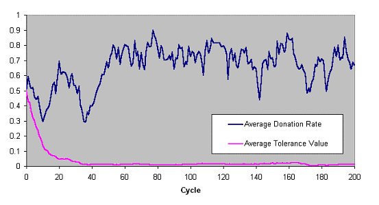
Figure 1. The average donation rate (the proportion of parings that resulted in a donation) and the average value of the tolerances across the whole population in a typical run of the Riolo et al. model (number of pairings=3 cost=0.1)

3.3
The interpretation that the Riolo et al. paper gave was that mutually cooperative groups of individuals with similar tags had evolved. Such groups arose so that all those in that group donated to others in that group and hence prospered compared to the rest of the population. Eventually, so their interpretation went, this group was 'invaded' by a non-donator who was a parasite in this group. This defector would then prosper faster than the co-operators until the group became all defectors when the advantage of being in the group would vanish and a new group based around a different tag range would arise.

3.4
Riolo et al claimed that the tolerance played a role similar to the defector/co-operator in the Prisoner's Dilemma problem. A very low tolerance indicated an individual who would not donate to many others (i.e. a defector) whilst an individual with a high tolerance would donate to others (i.e. a co-operator). They summarised their results as follows:
Strategies of donating to others who have sufficiently similar heritable tags ... can establish cooperation without reciprocity. (Riolo et al. 2001, page 443)

* Results From First Re-Implementation (Implementation A)

4.1
Below are the results from the first re-implementation of the Riolo model (in Java by David Hales). They are also over 30,000 time periods and 30 runs.

Table 3: Pairings is the number of times per generation each agent has an opportunity to donate to a randomly encountered other. The donation rate is the percentage of such encounters in which the choosing agent cooperates, that is, donates b = 1.0 at a cost of c = 0.1 to itself. The average tolerance is the average over all agents and all generations. The values in brackets show the difference between these results and the original results given in table 1


Effect of pairings on donation rate
PairingsDonation rate (%)Average tolerance
15.1 (3.0)0.010 (0.1)
242.6 (38.3)0.012 (0.5)
373.7 (0.1)0.018 (0.1)
476.8 (0.0)0.021 (0.0)
678.6 (0.1)0.023 (0.1)
879.2 (0.0)0.025 (0.0)
1079.4 (0.2)0.026 (0.2)


Table 4: The number of pairings is held at P = 3. The recipient benefit his held at b = 1 and the cost to the donor is varied as shown. The values in brackets show the difference between these results and the original results given in table 2

Effect of cost of donating on donation rate
CostDonation rate (%)Average tolerance
0.0573.7 (0.0)0.018 (0.001)
0.173.7 (0.1)0.018 (0.001)
0.273.7 (0.1)0.019 (0.001)
0.373.7 (0.2)0.018 (0.000)
0.461.0 (0.9)0.011 (0.000)
0.545.9 (21.2)0.008 (0.001)
0.68.1 (5.9)0.006 (0.001)

4.2
The results broadly agreed with those of the Riolo model, but the thresholds at which the high donation effect disappeared had shifted. In these results one was getting significant donation rates for only 2 pairings and for costs up to 0.5. It was at these thresholds that the re-implemented runs showed the greatest variance. With only a limited description and data in the original paper it is difficult to determine what the error was. For this reason the other author re-implemented the model in a different language (SDML[7]), to see if the Riolo et al. results could be implemented.

* Results from Second Re-implementation (Implementation B)

5.1
The results were only generated for 1 run up to 5000 generations and for up to 6 pairings (so confidence over results is lower than for the averages over 30 runs to 30,0000 generation so far) but they strongly indicate that the results match - although here we merely "eyeball" the results and intuit their similarity.

Table 5: Pairings is the number of times per generation each agent has an opportunity to donate to a randomly encountered other. The donation rate is the percentage of such encounters in which the choosing agent cooperates, that is, donates b = 1.0 at a cost of c = 0.1 to itself. The average tolerance is the average over all agents and all generations. The values in brackets show the difference between these results and the initial re-implementation results given in table 3


Effect of pairings on donation rate
ParingsDonation rate (%)Average tolerance
15.2 (0.1)0.011 (0.1)
242.6 (0.0)0.012 (0.0)
373.3 (0.4)0.018 (0.0)
476.6 (0.2)0.022 (0.1)
678.6 (0.0)0.023 (0.0)

* Validating that the Two Implementations were not Essentially Different

6.1
Simply "eyeballing" a few sets of results is not sufficiently tough test that two implementations are essentially the same - that the two are the same is a hypothesis which is amenable to statistical testing. However some care is needed in doing this - the nature of this simulation is that is can display several kinds of global behaviour that are very different in character and (in the medium term) self-reinforcing. Thus checking whether a medium scale sample of statistics from particular runs (e.g. average proportion of co-operators over time periods 100-200) is not productive since we would expect these to be from different distributions. However, if these implementations were the same one would expect that the averages of pretty well any statistic over all time periods collected over a number of independent runs from one implementation would come from the same distribution as those corresponding averages from the other implementation. Thus checking whether two such sets of averages do come from the same distribution using the two-sample Kolmogorov-Smirnov test (Chakravarti et al. 1967) is a test of the hypothesis that the implementations are the same in effect. We made the test even tougher by insisting that the two implementations pass this test simultaneously on a number of different output statistics and over a number different, and previously untried, parameterisations.

6.2
Thus what we did was:
  1. Take an untried set of values for the simulation parameters and set them as these in both implementations;
  2. Run both implementations over 1000 time periods collecting several different statistics from each time period;
  3. Calculate the averages of these statistics for each and record them;
  4. Do steps 2 and 3 an number of times (in our case 30) so that we have two sets of 30 numbers for each statistic gathered;
  5. For each such pair of sets of 30 numbers use the two-sample Kolmogorov-Smirnov test to give an estimate of the probability they come from the same distribution;
  6. Repeat steps 1 to 5 with different parameter settings.

6.3
Altogether his represents quite a tough test - the chances that the implementations would produce different statistics that came from the same shaped distribution over different and previously untried parameter settings is remote if they were essentially different. However, it does not prove[8] they are the same. There may well be a very different set of parameter settings and a new statistic where the results do not match in this way. One cannot prove that implementations are the same[9]; one can only do simulation experiments to try and disconfirm the hypothesis that they are the same. If such a hypothesis survives such repeated attempts then one can start to rely on it, but only within the ranges that it has been tested. It is always possible (indeed likely) that if one worked hard enough at it one would find critical settings where effectively chaotic aspects of a simulation meant that usually insignificant difference (e.g. the rounding method in the underlying arithmetic or the pseudo-random number algorithm) could be exploited to result in a measurable difference. If the set of such settings were either of a vanishingly small measure or only occurred with parameters of an extreme nature far from the range of concern then these can be safely ignored. This fits in with the Popperian view of science (Popper 1969).

* What do the results from the three implementations tell us?

7.1
Thus we had three models and three sets of results, so that two sets of results aligned but both disagreed with the published conceptual model and results. The situation is illustrated in Figure 2.

Figure 2
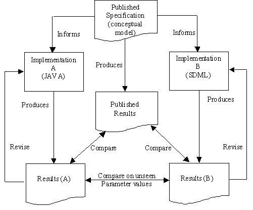
Figure 2. Relationship of published model and two re-implementations

7.2
Given that two independent implementations match each other but show significant differences from the original published results we speculated that there were three possible sources of the inconsistency:
  • The implementation used to produce the published results did not match the published conceptual model.
  • Some aspect of the conceptual model was not clearly stated in the published article
  • Both re-implementations had somehow been independently and incorrectly implemented (in the same way).

7.3
In some sense these points are not distinct issues but are very much related. It is essentially a matter of opinion as to the sufficiency and clarity of a natural language description of a "conceptual model" for the purposes of re-implementation. However, our argument is that if two independent re-implementations appear to make "the same mistake" then the problem is more likely to lay with the conceptual model description. This would seem to be especially true when the re-implementations align themselves even on previously unseen results from different parts of the parameter space.

* Three Variants Of Tournament Selection

8.1
In order to proceed we reconsidered the original natural language specification of the conceptual model given be Riolo et al. Where we found ambiguity we tried alternative implementations that conformed to the specification.

8.2
The problem of interpretation was identified in the tournament selection procedure for reproduction. In the original paper it is described thus:
After all agents have participated in all parings in a generations agents are reproduced on the basis of their score relative to others. The least fit, median fit, and most fit agents have respectively 0, 1 and 2 as the expected number of their offspring. This is accomplished by comparing each agent with another randomly chosen agent, and giving an offspring to the on with the higher score.

8.3
It turned out that in both re-implementations (A and B) the authors had assumed that when an agent has an identical score to a randomly chosen agent then a random choice is made between them to decide which to reproduce into the next generation (since this is left unspecified in the text). However, when a comparison was made of alternative re-implementations with different reproduction rubrics (when both agents have the same score) it was found that the original implementation must have incorporated a bias towards the systematically selected agent (not the randomly selected agent).

8.4
Let us be clearer now (with pseudo-code) as to the three different possible rubrics of reproduction we implemented. Table 6 gives outline algorithms for each of the three rubrics that were implemented.

Table 6: Outline pseudo-code algorithms for the three different tournament selection methods tested

Three Variants Of Tournament Selection
LOOP for each agent in population
  Select current agent (a) from pop
  Select random agent (b) from pop
  IF score (a) > score (b) THEN
   Reproduce (a) in next generation
  ELSE IF score (a) < score (b) THEN
   Reproduce (b) in next generation
  ELSE (a) and (b) are equal
   Select randomly (a) or (b) to be
   reproduced into next generation.
  END IF
END LOOP
LOOP for each agent in population
  Select current agent (a) from pop
  Select random agent (b) from pop
  IF score (a) >= score (b) THEN
   Reproduce (a) in next generation
 ELSE score (a) < score (b)
  Reproduce (b) in next generation
 END IF
END LOOP
LOOP for each agent in population
  Select current agent (a) from pop
 Select random agent (b) from pop
 IF score (a) <= score (b) THEN
   Reproduce (b) in next generation
  ELSE score (a) > score (b)
   Reproduce (a) in next generation
  END IF
END LOOP
(a) No Bias(b) Selected Bias(c) Random Bias

8.5
That is in each of these three cases, if the scores of the two selected individuals are different then the individual with the higher score gets reproduced into the next generation. The three algorithms only differ in the case where the scores happen to be exactly the same. In this, equal, case: in the no bias algorithm a random individual is reproduced; in the selected bias case the individual is reproduced; and in the random bias case the individual it was paired with is reproduced. The difference between the last two is subtle: if all the scores of the population were the same then in the selected bias case each individual would be reproduced once into the next generation, whilst in the random bias case it would be the random selection that would be reproduced. As you can see it is far from obvious that such differences would have any significant effect on the results of the simulation.

8.6
It was found that the authors of both re-implementations had independently assumed that the "no bias" algorithm (Table 6a) was the correct interpretation of the natural language description given in the original published article (see above). However, it was determined that the "selected bias" algorithm (Table 6b) reproduced the results given. Hence it would appear that Riolo et al, used the "selected bias" method and that this was the reason for the different results obtained from the two previous re-implementations. Tables 7 and 8 show results for each of the algorithms given in Table 6. It is worth noting that the "selected bias" method almost perfectly matches the published results but that this method produces different results from the other two ("no bias" and "random bias") methods.

Table 7: Here we compare the results of donation rates (Don) and average tolerances (Ave. Tol) for each of the three different tournament selection algorithms described in table 6 over different "pairings" values. We note that the "selected bias" method very closely matches the published results from the initial model (given in table 1). As before the results are calculated from 30 independent runs to 30,000 generations.

Results From the Three Variants of Tournament Selection
No Bias (a)Selected Bias (b)Random Bias (c)
PairingsDonAve. TolDonAve TolDonAve Tol
15.10.0102.10.0096.00.010
242.60.0124.40.00749.60.013
373.70.01873.70.01973.70.018
476.80.02176.90.02176.80.021
678.60.02378.60.02378.70.023
879.20.02579.20.02579.20.025
1079.40.02679.40.02679.40.026


Table 8: Here we compare the results of donation rates (Don) and average tolerances (Ave. Tol) for each of the three different tournament selection algorithms described in table 6 over different donation cost values. We note that the "selected bias" method very closely matches the published results from the initial model (given in table 2). The results are calculated from 30 independent runs to 30,000 generations

Results from the Three Variants of Tournament Selection
No Bias (a)Selected Bias (b)Random Bias (c)
CostAve. DonAve. TolAve DonAve TolAve DonAve Tol
0.0573.70.01873.60.01873.70.018
0.173.70.01873.70.01973.70.018
0.273.70.01973.70.01973.70.018
0.373.70.01873.60.01973.70.018
0.461.00.01160.50.01161.00.011
0.545.90.00826.20.00746.70.008
0.68.10.0062.10.0059.90.006

* Further investigations into the published model

9.1
We had now successfully re-implemented the published conceptual model in two different ways so that they reproduced the published results and were aligned with each other. This gave us confidence that we had implementations that correctly aligned with those that Riolo et al. described in their paper. We could now investigate the full properties of this implemented model, beyond those described.

9.2
Although the model was fairly robust with respect to the number of pairings and the cost, we found that the model was far from robust in other ways. In the published model donation occurred if the difference in tag values (of donor and recipient) was less than or equal to the tolerance of the donor (| tD-tR | ≤ TD). This meant that if the tags of the donor and recipient were exactly the same (what we call 'tag clones'), then the donor must always donate, since | tD-tR | = 0 and TD ≥ 0 by the construction of the simulation. It was found that if the condition for donation was changed to | tD-tR | < TD (i.e. the difference in tag values is strictly less than the tolerance) then the high donation rates achieved in the Riolo model vanished. Table 9 and Table 10 show the corresponding results in this case.

Table 9: Here are the results when all parameters are identical to those used in Table 1 (i.e. the original published results) except that donation only occurs when the differences in tags is strictly less than (rather than less then or equal to) tolerance. As can be seen, donation is completely wiped out


Effect of pairings on donation rate (strict tolerance)
ParingsDonation rate (%)Average tolerance
10.00.000
20.00.000
30.00.000
40.00.000
60.00.000
80.00.000
100.00.000


Table 10: Results obtained when all parameters are identical to those used in Table 2 (i.e. the original published results) except that donation only occurs when the differences in tags is strictly less than (rather than less then or equal to) tolerance. As can be seen, donation is completely wiped out

Effect of cost of donating on donation rate (with strict tolerance)
CostDonation rate (%)Average tolerance
0.050.00.000
0.10.00.000
0.20.00.000
0.30.00.000
0.40.00.000
0.50.00.000
0.60.00.000

9.3
Figure 3 is the equivalent of Figure 1 for this case. You can see how the donation rate disappears down to zero after the initial period. All the agents have evolved zero or near-zero tolerances and no group of mutual donators has appeared.

Figure 3
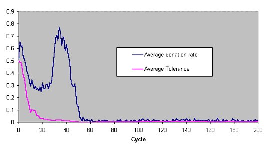
Figure 3. The average donation rate (the proportion of pairings that resulted in a donation) and the average value of the tolerances across the whole population in a typical run of the Riolo et al. model (number of pairings=3 cost=0.1) but with strict tag comparisons.

9.4
In this case, where individuals can evolve so that they are not forced to donate to tag clones of themselves the emergent 'altruism' does not occur and tolerances quickly go to zero. Further experimentation revealed that the effect reported in (Riolo) was due to the fact that the simulation quickly becomes dominated by a single group of individuals, all of whom have exactly the same tag. Once such a group is established there is a high probability that individuals in this group will be paired with each other and thus donate to each other. The individuals are thus likely to have a higher score that those not in this group, so they are preferentially reproduced into the next generation which reinforces the group. This is completely contrary to the impression they give in their paper which is a dynamic one of many groups arising and being invaded by defectors.

9.5
The figures below illustrate what is happening for the reader. Figure 4 is a histogram over time of the frequency of tag value occurrence over the first 200 generations. The total range of values is divided into 100 intervals (0-0.01, 0.01-0.02, ..., 0.99-1), the number of tag values in each is counted and plotted against time. Since this is difficult to understand in detail, in Figure 5 shows the significant detail from this. You can see that after some competition in the first 60 generations a single interval dominates.

Figure 4
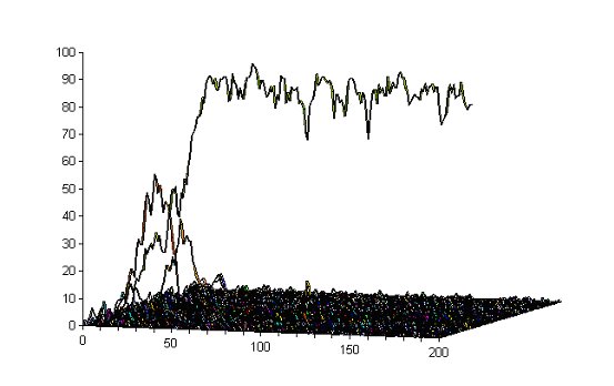
Figure 4. The frequency histogram of each interval of 0.01 (0-0.01, 0.01-0.02 etc.) over the first 200 generations in the typical run illustrated above in Figure 1 (the Riolo et al. model with 3 pairings and cost of donation at 0.1), i.e. each 'line' shows how many individuals have a tag in that range in that generation. Significant detail from this is shown in Figure 5 immediately below

Figure 5
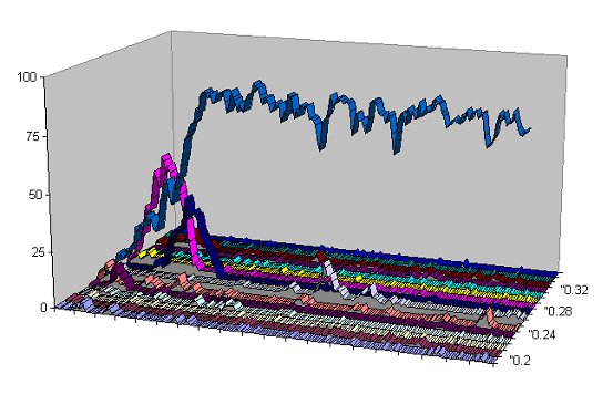
Figure 5. Detail from Figure 4 showing the frequency of tag values over time for the intervals 0.02-0.021, 0.021-0.022, ..., 0.034-0.035 for the first 200 generations

9.6
In fact in this interval a single tag value dominates, although this is cannot be seen from the histogram. Within this single interval individuals with a zero tolerance form a significant proportion, as is shown in Figure 6. Here individuals with zero tolerance can be seen to form a substantial core of the dominant tag group. Due to the operation of mutation there will always be a 'penumbra' of individuals in the group with small but non-zero tolerances due to the 'pressure' of the tolerance mutation - 10% of the core will become part of the 'penumbra' each generation due to this feature of the model.

Figure 6
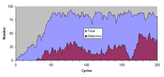
Figure 6. The total frequency of tag values in the dominant interval and the number of these that have a zero tolerance value (called defectors here since they only donate to others with an identical tag) over the first 200 generations

9.7
We hypothesised that the Riolo et al. model only worked because this dominant core of zero-tolerance tag-clones had to donate to each other. To test this we also ran versions of the Riolo model where all the tolerances were set permanently to zero. The results of this are shown in Table 11and Table 12 below. These tables show the results for each of the selection methods shown in Table 6.

Table 11: Results when tolerance is forced to be always zero for all agents (i.e. the tolerance mechanisms is turned-off) with all other settings as they were for the original results given in Table 7

Results when tolerance set to zero for different Pairings
No Bias (a)Selected Bias (b)Random Bias (c)
ParingsDonAve. TolDonAve TolDonAve Tol
13.10.0000.00.0004.10.000
265.40.0000.00.00065.60.000
375.30.0000.00.00075.40.000
477.60.0000.00.00077.70.000
678.80.0000.00.00078.80.000
878.90.0001.90.00078.90.000
1079.00.0007.60.00079.00.000


Table 12: Results when tolerance is forced to be always zero for all agents (i.e. the tolerance mechanisms is turned-off) with all other settings as they were for the original results given in Table 8

Results when tolerance set to zero for different Costs
No Bias (a)Selected Bias (b)Random Bias (c)
CostAve. DonAve. TolAve DonAve TolAve DonAve Tol
0.0575.30.0000.0000.00075.40.000
0.175.30.0000.0000.00075.40.000
0.275.30.0000.0000.00075.40.000
0.375.30.0000.0000.00075.40.000
0.466.00.0000.0000.00066.00.000
0.559.70.0000.0000.00059.80.000
0.617.20.0000.0000.00020.30.000

9.8
In these tables we see an interesting (and initially unexpected) result - notice that for the selected bias results we get low donation rates but it is high for both other selection mechanisms. Why is this? Reflection on the nature of the selection mechanisms (see Table 6) offers an explanation for the seemingly anomalous results.

9.9
Consider an initial population of 100 agents each with a randomly assigned tag (so almost certainly each agent will have a unique tag value). With tolerance set to zero, and no shared tag values, agents will not donate to other agents - they will never find a partner matching their tag. This means all agents will obtain a score of zero. Using the selected bias mechanism when all agents have the same score will produce the result that the next generation will consist of the same agents as the previous generation with some mutation applied to tags. However tag mutation (either a new tag is assigned with probability 0.1 or the tag is left unchanged) is unlikely to produce agents with matching tags. Consequently there is no scope for groups of "tag clones" to form because there is no chance for agents to produce more than a single copy of themselves into the next generation. This then, implies that all the cooperation we have seen in all runs of the model is a result of agents donating between tag clones (which is built into the assumption of the model - remember agents have to donate to tag clones). This ties in with the previous results showing that donation disappears when the difference between tags must be strictly less than the tolerance (Table 10)[10].

9.10
In the other selection cases there is a chance that an agent may get replicated more than once into the next generation. Now, if we wished to verify that the tolerance mechanism was significant in producing high donation and only results from the selected bias method were examined it would superficially appear that the tolerance mechanism was driving high donation because when it was turned off donation appears to disappear. However, as we see here, the two other selection mechanisms show that this is not the case. This is important because the original results ascribe the donation process to the tolerance process, not the particular (and rather peculiar) specific selection process. The generalisation then, of those original results to general evolutionary process would appear to be false[11]. In this sense it's hard to accept the social interpretations of the world as originally published (Riolo et al. 2001, and the commentary of Sigmund and Nowak 2001). We note here that, as a direct result of multiple re-implementations, deeper insight has been gained into important (and previously hidden) aspects of the model which have major implications with respect to possible interpretations of the results.

9.11
As can be seen in Table 11 and Table 12 the general effect of high donation rates remains in the complete absence of the tolerance mechanism for the no bias and random bias selection methods. As stated above, this is due to both these mechanisms allowing for the chance that an agent may make more than one copy of itself to the next generation (and hence producing a tag clone group).

9.12
It could be argued at this stage that the tolerance mechanism might become operative if agents were not allowed to produce clones. So that although the model and results so far are not sufficient to demonstrate a tolerance process promoting cooperation it could work. To test this hypothesis we produced a further simulation in which we introduced a very small but certain mutation of tag values (Gaussian noise with mean zero and standard deviation of 10-6) into the reproduction process so that a group could never exactly clone itself[12]. In this case the tolerance mechanism would have to come into play if a high donation rate was to emerge. But the high donation effect vanished again (see Table 13 and Table 14).

9.13
Finally, to see whether the reported effect was robust to changes in population size we ran the simulations with twice the population size (i.e. 200 individuals). Again the donations rates vanished (we have not reproduced these tables since they are identical to Table 9 and Table 10 above).

9.14
In this manner we were able to understand how the published model was dependent upon the forced donation among tag clones and that the tolerance mechanism was essentially irrelevant.

9.15
It seems that we now understand the published model better than the original authors. A more informative and precise summary of their paper could be:
Compulsory donation to others who have identical heritable tags can establish cooperation without reciprocity in situations where a group of tag clones can replicate themselves exactly
- which is a somewhat less significant result that that claimed in the original paper.

Table 13: Results when a very small level of Gaussian noise is added to the tag value during the replication process (when an agent is copied into the next generation). Notice that the donation rate drops sharply[13] (over Table 7) - this would not happen if the originally published interpretation held

Results when noised added to tag values on reproduction
No Bias (a)Selected Bias (b)Random Bias (c)
PairingsDonAve. TolDonAve TolDonAve Tol
13.70.0091.90.0094.20.009
23.10.0071.50.0063.70.007
34.00.0051.50.0055.10.005
46.80.0052.00.0058.50.005
613.10.0046.20.00414.20.004
815.50.00412.70.00416.20.004
1012.10.00210.90.00312.80.003


Table 14: Results when a very small level of Gaussian noise is added to the tag value during the replication process (when an agent is copied into the next generation). Notice that the donation rate drops sharply (over Table 8) - this would not happen if the originally published interpretation held

Results when noise added to tag values on reproduction
No Bias (a)Selected Bias (b)Random Bias (c)
CostAve. DonAve. TolAve DonAve TolAve DonAve Tol
0.054.00.0061.50.0055.10.005
0.14.00.0051.50.0055.10.005
0.23.90.0051.40.0055.00.005
0.34.00.0051.40.0055.20.006
0.43.20.0051.30.0053.80.005
0.52.70.0051.30.0053.20.005
0.62.50.0051.20.0052.90.005

* Some practical lessons about aligning models

10.1
Here we briefly describe some of the techniques and tips we have learnt that aid the alignment of simulations.
  • Check the alignment of simulations in the first few time cycles of their runs (possibly averaged over several runs). This indicates whether they are initialised in the same way and the differences may be clearer than after new, self-reinforcing, effects emerge in the simulation or chaos appears.
  • Use statistical tests over long-term averages of many runs, using such as the Kolmogorov-Smirnov test (Chakravarti et al. 1967) to see whether two sets of figures come from the same distribution. Often sets of figures that look the same fail this sort of test.
  • If two simulations do not align, progressively turn off features of the simulation (e.g. donation, reproduction, mutation etc.) until they do align. Then search for the differences in the reduced model. Then progressively reintroduce the features.
  • Use different kinds of languages to re-implement a simulation (we used a declarative and an imperative language) and, if possible, programmed by different people. Failing that, at least use different kinds of program or data structure. Otherwise there is a good chance that any mistakes or assumptions will simply be repeated in both.

* Discussion

11.1
In this paper we have characterised a simulation as a (formal but non-analytic) computational theory[14], which can effectively be checked only via experiment. Each simulation run corresponds to such an experiment.

11.2
Give this approach to simulations, much of the established scientific practice on conducting experiments can be applied including:
  • That there should be a norm concerning the publication of simulation results, namely that the description of the simulation should be sufficient for others to be able to replicate (i.e. re-implement) the simulation;
  • That experiments have to be independently replicated by others and the results confirmed before the simulation or the results are taken seriously;
  • That simulations can not be confirmed as correct by any number of runs but merely survive repeated attempts at refutation, and thus gradually come to be relied upon (Popper 1969);
  • That it is often more productive if runs of a simulation are directed at particular hypotheses about the simulation process rather than aim to be generally indicative - this has the advantage that data can be collected in a focused way to suit the issue being simulated rather than try to fit the simulation to what data happens to be available.

11.3
The difficulties of model alignment are highly suggestive of the difficulties of modelling social phenomena. In model alignment one is attempting to model one simulation with another. To do this alignment one has all the possible advantages: any detail of the target simulation is potentially inspectable; all experiments are repeatable; the design of the target simulation is known and is not extremely complex; the simulations will be partly modular, allowing some features to be tested separately[15]. When modelling observed social phenomena one does not have these advantages - if aligning one computational model against another is hard, how much more so must be truly aligning a computational model with a real world social process!

* Conclusions

12.1
If we had not re-implemented the Riolo model we would not have been able to discover its shortcomings. If we had not re-implemented the model in two independent ways we would not have been able to state with confidence that the shortcomings were inherent in the original model rather than ours. Further, the double re-implementation greatly aided us in finding simulations that aligned with the original. In other words, without double re-implementation, there would have been a distinct possibility that the shortcomings would never have come to light.

12.2
Since almost all simulations are not amenable to formal analysis, the only way they can be verified is via the experimentation of running simulations. If we are to be able to trust the simulations we use, we must independently replicate them. An unreplicated simulation is an untrustworthy simulation - do not rely on their results, they are almost certainly wrong[16].

* Acknowledgements

We would like to thank the participants of the "Model to Model" workshop for their perceptive comments and questions during and after the M2M workshop. We would also like to thank the M2M reviewers whose comments were invaluable and helped us to improve our paper. We would also like to thank GREQAM-CNRS in Marseilles for their support for the M2M workshop.


* Notes

1 There is some confusion about the terminology of "model" - see (Edmonds 1999), chap 2.

2 Unfortunately, in many papers the conceptual model is not explicitly delineated; a causal reading might lead one to believe the simulation was directly about the observed phenomena (Edmonds 2000)

3 Of course, there could be problems with both aspects (when specifications are vague and implementations complex).

4 Several recent models and investigations have shown how "tags" (arbitrary social cues) can catalyize group level self-organisation from previously disparate individuals (Hales 2001, Hales 2002a, Hales 2002b, Hales and Edmonds 2002).

5 We say "seemingly" because not all is what it may first appear - the process of re-implementations here described uncovered some interested issues concerning the model (but more of this later).

6 Strictly speaking they are not groups but this term provides a more vivid picture of what occurs.

7 See http://sdml.cfpm.org

8 Using a (unrealistically strong) philosophical sense of "prove" here.

9 In extremely simple cases (no real numbers, no random component, no input from outside world, very simple algorithms etc.) it has been possible to effect a machine verification with respect to formal specification, but this is not possible with any simulation of the kind we are talking about.

10 Indeed further statistics recording the proportion of donation events the occur between non-tag-clone agents were collected, these were always almost zero.

11 When the model was implemented with a probabilistic roulette wheel selection algorithm (where reproductive success is probabilistically and proportionally related to fitness - or score in this case) results similar to the random bias results were produced.

12 This is in addition to the 10% chance of having the tag value reset - which remains unchanged.

13 Notice also the non-monotanicity in the donation rates - indeed further runs examining 20 and 40 awards showed even lower donation rates. This interesting phenomenon is beyond the scope of this paper and may be addressed in future papers.

14 The implemented simulation is usually a particular case of the conceptual model which is more generally applicable but less precise.

15 Even then the chaotic nature of some of the processes may mean that complete alignment is impossible. These difficulties imply that, often, it may not be possible to separate out the theory that the simulation is supposed to embody and the implementation.

16'Wrong' in the sense that, at least in some detail or other, the implementation differs from what was intended or assumed by the modeller.

* Appendix

References and Sources

The original discussion of tags in the context of artificial social processes and models is Holland (1993). The model in this paper is based around (variations of) Riolo et al. (2001). David Hales has written quite a few papers on tag mechanisms and models - these are all accessible from either http://www.davidhales.com or as CPM-reports at http://cfpm.org/cpmreports.html.

Static structure

The model has 100 agents. Each agent has two (inheritable) characteristics: a tag (a floating point in [0,1]) and a tolerance (a floating point in [0,1]).

Dynamic structure

Each simulation has is divided up into a finite number of discrete time periods (called 'generations'). Each generation is divided up into a number of phases:
  • Creation / replication of new population from the old;
  • Pairing and donation - for each agent in the population;
  • Summing up the fitness scores;
  • Reporting and statistics.

The only permanent variables that change are the tag and tolerance values for each of the 100 individuals. Temporary variables (that only have effect within a generation) are the donations and the fitness scores).

Key parameters and options

The parameters of the standard set-up (following Riolo et al) are as follows, (their value or range of values are in brackets).
  • The population (100);
  • The range for tag values ([0, 1]);
  • The range for tolerance values ([0, 1])
  • The number of generations the simulation is run for (30,000);
  • The number of runs (30);
  • The number of other agents each agent is 'paired with' for potential donation, P, (1, 2, 3, 4, 6, 8, 10);
  • The cost to an agent of making a donation, c (0.05, 0.1, 0.2, 0.3, 0.4, 0.5, 0.6);
  • The benefit gained from receiving a donation (1);
  • The probability of tag mutation (0.1);
  • The probability of tolerance mutation (0.1);
  • The standard deviation of the Gaussian noise added to tolerance during mutation (0.01);
  • The standard deviation of the Gaussian noise that is always applied to the tag value during reproduction (0).

In Riolo et al. (2001) only c, the donation cost, and P, the number of pairings, are varied. In this paper the following are never varied: the population, the tag range, the probability of tag or tolerance mutation; or the standard deviations of the tolerance mutation Gaussian noise.

Key algorithm options are:

  • Which agent is selected for reproduction when fitness scores are equal: the selected one - 'selected bias'; the one it was compared with - 'random bias'; a random choice between these - 'no bias' (selected bias);
  • Whether | tD - tR | ≤ TD - 'non-strict' comparison; or | tD - tR | < TD - 'strict' comparison is used to determine whether a donation takes place (non-strict).

The algorithm (standard version)

For each generation
	For each agent, a
		 Randomly select another different agent, b
		If total score of b is strictly greater than the total score of a (selected bias)
		Then replace a with b
		Else keep a
	Next agent
	For each agent, a
		With probability 0.1 replace its tag with a new random value in [0, 1]
		With probability 0.1
			Add Gaussian noise (mean 0 sd 0.01) to tolerance
			If tolerance less 0 set to 0, if greater 1 set to 1
		Reset a's score to zero
	Next agent
	For each agent, a
		 Randomly select another different agent, b
		If +ve difference of (tag of a) and (tag of b) < (the tolerance of a)
				(strict comparison)
		Then add 1 to score of b and subtract c from score of a
	Next agent
Next generation

Initialisation

At the start of the first generation, the agents were initialised with all tag values and tolerance values being uniformly randomly selected from the interval [0, 1]. All values were independently drawn in each run of the simulation.

Intended interpretation

Riolo et al. gave the following interpretation to their simulation:
Strategies of donating to others who have sufficiently similar heritable tags ... can establish cooperation without reciprocity.
As a result of our investigations we give it a more restricted interpretation:
Compulsory donation to others who have identical heritable tags can establish cooperation without reciprocity in situations where a group of tag clones can replicate themselves exactly.

Details necessary for implementation but not thought to be critical to the results

The exact selection method did not seem to make a lot of difference to the results as long as it allows the occurrence of random drift in an initial random population, otherwise the process of donation and 'group' formation will not get started. Likewise as long as there is some mechanism to cause initial 'proto-groups' (more than one individual with the same tag) to form almost any initial population will do, it does not need to be random. The ranges for the tags and the tolerances are essentially arbitrary and could be any limits. The exact cost/scoring mechanism is probably not critical as long as mutually donating groups do better than others and so are preferentially replicated. In other papers we have found that (unlike in the model investigated here) tag-based mechanisms can be robust over a wide range of conditions, but these conditions are only starting to be sketched out (see David Hales' papers on this athttp://www.davidhales.com).

Description of variations

The standard set-up is as described as above (especially the sub-section on 'Key parameters and options' above). The variations explored are as follows.
Version with the 'no bias' selection method
This is the same as the standard version except that the 'no bias' selection method is used.
Version with the 'random bias' selection method
This is the same as the standard version except that the 'random bias' selection method is used.
Version with strict tag comparison
This is the same as the standard version except that 'strict' tag comparison is used to determine whether there will be a donation each time a pairing occurs.
Version with fixed zero tolerances
This is the same as the standard version except that the range for tolerances is [0, 0] - i.e. the tolerances are fixed to zero and that each of the three selection methods are applied.
Version with non-exact reproduction
This is the same as the standard version except that the standard deviation for the Gaussian noise in all reproduction is set to 0.000001.

Software Environment

The model was implemented in two languages Java - and Object-oriented language developed by Sun (see http://java.sun.com) and SDML - a declarative forward chaining programming language which has been written specifically for agent-based modelling in the fields of business, management, organization theory and economics (see http://sdml.cfpm.org and Moss et al 1998). The pairing was particularly useful for while SDML was excellent for exploring and understanding the results and emergent processes Java was suitable for performing the 30 runs to 30,000 generations to match the results in Riolo et al. (2001).

Code

The modules with the code for this simulation will be available at URL: http://cfpm.org/replication/riolo. The SDML modules require SDML version 4.1. SDML is freely available for academic use, it can be acquired from URL: http://sdml.cfpm.org (although at the moment there seems no prospect of being able to actively maintain the language). The Java ".jar" files require the Java2 1.3 runtime environment (or higher) see http://java.sun.com.

Raw Results

The raw statistics are far too bulky to store on a server. However we hope that shortly the model will be able to be remotely run and the results queried from our AgentCities server 'Intelligent Simulation Models' from the web page http://cfpm.org/ism

* References

DAVID, N., Sichman, J. and Coelho, C. (2002), Towards an Emergence-Driven Software Process for Agent-Based Simulation. 3rd International Workshop on Multi-Agent Based Simulation (MABS). Bologna, Italy, July 2002. Lecture Notes in Artificial Intelligence, 2581.

CHAKRAVARTI, Laha, and Roy, (1967), Handbook of Methods of Applied Statistics, Volume I, John Wiley and Sons, pp. 392-394.

EDMONDS, B. (1998), Social Embeddedness and Agent Development. UKMAS'98, Manchester, December1998. (available at: http://cfpm.org/cpmreps.html ).

EDMONDS, B. (1999), Syntactic Measures of Complexity. Philosophy. Manchester, University of Manchester. (available at: http://bruce.edmonds.name/thesis).

EDMONDS, B. (2000), The Use of Models - making MABS actually work. In Moss, S., Davidsson, P. (Eds.) Multi-Agent-Based Simulation. Lecture Notes in Artificial Intelligence, 1979:15-32. Berlin: Springer-Verlag.

ENGELFRIET, J. Jonker, C. and Treur, J. (1999), Compositional Verification of Multi-Agent Systems in Temporal Multi-Epistemic Logic. In Proceedings of the 5th International Workshop on Intelligent Agents V : Agent Theories, Architectures and Languages (ATAL-98), Springer. Lecture Notes in Artificial Intelligence 1555:177-194.

HALES, D. (2000), Cooperation without Space or Memory: Tags, Groups and the Prisoner's Dilemma. In Moss, S., Davidsson, P. (Eds.) Multi-Agent-Based Simulation. Lecture Notes in Artificial Intelligence, 1979:157-166. Berlin: Springer-Verlag.

HALES, D. (2001), Tag Based Cooperation in Artificial Societies. Ph.D. Thesis, Department of Computer Science, University of Essex (available at: http://www.davidhales.com/thesis).

HALES, D. (2002a), 1. Evolving Specialisation, Altruism and Group-Level Optimisation Using Tags. In Sichman, J. S., Bousquet, F. Davidsson, P. (Eds.) Multi-Agent-Based Simulation II. Lecture Notes in Artificial Intelligence 2581:26-35 Berlin: Springer-Verlag.

HALES, D. (2002b), Smart Agents Don't Need Kin - Evolving Specialisation and Cooperation with Tags. CPM Working Paper 02-89. The Centre for Policy Modelling, Manchester Metropolitan University, Manchester, UK (available at: http://cfpm.org/cpmreps.html).

HALES, D. & Edmonds, B. (2002) Evolving Social Rationality for MAS using "Tags". CPM Working Paper 02-104. The Centre for Policy Modelling, Manchester Metropolitan University, Manchester, UK (available at: http://cfpm.org/cpmreps.html).

HOLLAND, J. (1993), The Effect of Labels (Tags) on Social Interactions. SFI Working Paper 93-10-064. Santa Fe Institute, Santa Fe, NM. (available at: http://www.santafe.edu/sfi/publications/wplist/1993)

MORGAN, M. and Morrison, M. (2000) Models as Mediators, Cambridge University Press.

POPPER, K. R. (1969) Conjectures and Refutations. London: Routledge & Kegan Paul.

RIOLO 2001"> RIOLO, R. L., Cohen, M. D. and Axelrod, R (2001), Evolution of cooperation without reciprocity. Nature, 411:441-443.

SIGMUND, K. and Nowak, M. A. (2001), Evolution - Tides of tolerance. Nature 414:403.

----

ButtonReturn to Contents of this issue

© Copyright Journal of Artificial Societies and Social Simulation, [2003]