
Andreas Flache and Rainer Hegselmann (2001)
Do Irregular Grids make a Difference? Relaxing the Spatial Regularity Assumption in Cellular Models of Social Dynamics
Journal of Artificial Societies and Social
Simulation vol. 4, no. 4
<https://www.jasss.org/4/4/6.html>
To cite articles published in the Journal of Artificial Societies and Social Simulation, please reference the above information and include paragraph numbers if necessary
Received: 4-July-01 Accepted: 10-Sep-01 Published: 31-Oct-01
 Abstract
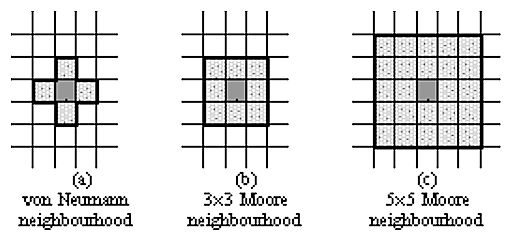 |
| Figure 1: Neighbourhood definitions in a cellular automaton. |
Irregular Grids in a Cellular
Automaton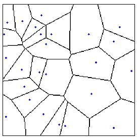 |
| Figure 2: A Voronoi diagram. |
 |
| Figure 3: Cells with 3, 4, 5, and 8 next neighbours in a Voronoi graph. |
The Dynamics of Reciprocity in
Irregular Worlds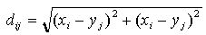 , where
(xi , yi) and (xj ,
yj) represent the generator coordinates. The neighbourhood of a
cell then includes those cells that lie within a maximal distance r from
the focal cell. This distance may represent the physical properties of the
pollution process. In particular, it implies that the side effects of the
pollution of a particular individual can no longer be felt, if the distance to
this individual exceeds the maximum range r. Throughout this paper we
assume that points in the rectangle in which cells are embedded are described
in a two-dimensional euclidian space with coordinates of 0...1000 × 0..1000.
Moreover, in all models the cellular world is a torus, i.e. it has no borders.
Cells that appear in a 2-dimensional representation of the grid on the left
border are neighbours of cells that appear on the right border and cells that
appear on the upper border are neighbours of those that appear on the lower
border, and vice versa.
, where
(xi , yi) and (xj ,
yj) represent the generator coordinates. The neighbourhood of a
cell then includes those cells that lie within a maximal distance r from
the focal cell. This distance may represent the physical properties of the
pollution process. In particular, it implies that the side effects of the
pollution of a particular individual can no longer be felt, if the distance to
this individual exceeds the maximum range r. Throughout this paper we
assume that points in the rectangle in which cells are embedded are described
in a two-dimensional euclidian space with coordinates of 0...1000 × 0..1000.
Moreover, in all models the cellular world is a torus, i.e. it has no borders.
Cells that appear in a 2-dimensional representation of the grid on the left
border are neighbours of cells that appear on the right border and cells that
appear on the upper border are neighbours of those that appear on the lower
border, and vice versa.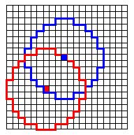
| Figure 4: Neighborhood of two individuals in the rectangular cellular world (r=300, cellsize 50 × 50). |
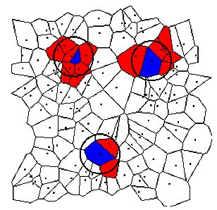 |
| Figure 5: Neighbourhoods of three different cells in an irregular grid. Range r = 100, 11 × 11 cells. Focal cells are blue, neighbour cells are red. |
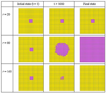 |
| Figure 6: Non-linear effects of neighbourhood size r in a rectangular torus world. Expectation level E = 30%, Initial cluster of 9 × 9 = 81 contributors, 50 × 50 torus grid. |
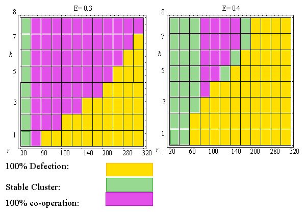 |
| Figure 7: Effects of expectation level E, cluster size h and neighbourhood radius r on final state of TFT-dynamics. Rectangular grid. |
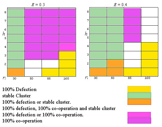 |
| Figure 8: Effects of expectation level E, Cluster size h and neighbourhood radius r on final state of TFT-dynamics. Rectangular grid with varying location of cluster. |
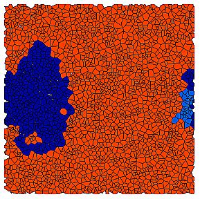 |
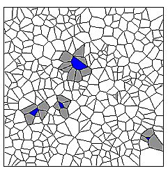
| Figure 9: Path dependence in the growth of a cluster in an irregular grid. Colours indicate relative frequency of co-operation in this cell in the endstate, based on 100 replications. Dark blue = 100%, Blue = 83%, Red = 0%). Initial cluster size h = 190, expectation level E = 0.3, neighbourhood size r = 30. |
 [1]
[1]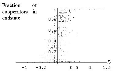 |
| Figure 10: Fraction of co-operators in the endstate as a function of the relative density of the initial cluster. E = 0.3, r = 50 and h = 30. Results are based on 2500 different cluster locations and 50 replications per condition. |
Backward-looking Social Support in
Irregular Worlds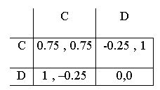 |
| Table 1: Payoffs of the constituent support game. |
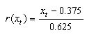 [2]
[2]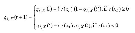 [3]
[3]
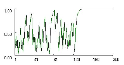 |
| Figure 11: Change in propensities for co-operation in dyadic support game simulated with the Bush Mosteller stochastic learning algorithm and high learning rate l = 1. |
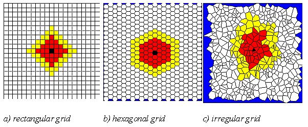 |
| Figure 12: Migration windows with radius 3 (red) and 5 (yellow) around focal cell (black) in 3 different grid structures. |
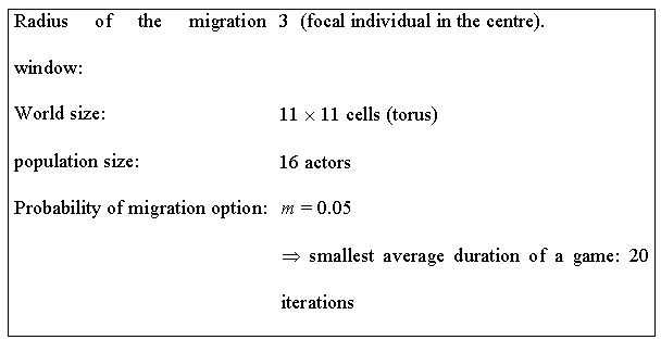 |
| Table 2: Main assumptions of simulation of migration dynamics. |
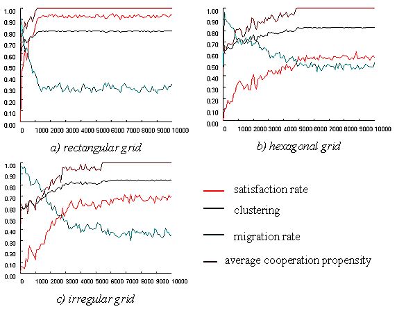 |
| Figure 13: Dynamics of co-operation and migration in three different grid structures. |
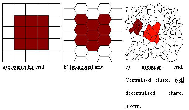 |
| Figure 14: Structures of 3 × 3 clusters in three different grids. |
Conclusions2For the mathematical details see Okabe et al. (1992). Details of our implementation of Voronoi-diagrams and some sample data sets can be found on our website.
3With exception of the four corner members of the cluster, who change into defectors, because they see only 25% co-operation around them, less than their expectation level E. However, the conversion of these four cells is more than outweighed by the changes from defection to co-operation.
4With this assumption, the support game used here is different from the support game used in Hegselmann and Flache (1998). The main difference is that bilateral help is always possible in the game we use here, though the degree varies for different neediness class combinations. By contrast, the support game of Hegselmann and Flache (1998) allows in each period only unilateral help. As a consequence, that game imposes imperfect information which greatly complicates the game theoretical analysis. Obviously, there are different plausible approaches to model what in the daily life is simply called mutual help.
5This implementation of the learning dynamics is different from an alternative formalization of the "power law of practice" that was proposed by Erev et al (1999). Flache and Macy (2001) showed that for parameter values corresponding to those used in the present paper, both models generate very similar behaviour. However, the authors also reveal subtle but important differences that occur in other regions of the parameter space, in particular when actors’ aspiration levels are high or their learning rates are low.
6To recall, we define a next neighbour as a cell that has a common border with the focal cell. For the rectangular world, this imposes a von Neumann neighborhood structure.
7Simultaneously, the opponent adapts her corresponding attractiveness assessment. The sequence in which dyads are selected is randomly chosen.
8More precisely, we assume that a particular
player i assesses the attractiveness payoff attained in interactions
with others after the t'th encounter as: 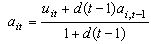 .
The symbol uit indicates the payoff attained at the
t'th encounter and ai,t-1 is the estimate of others'
attractiveness before the t'th encounter occurred. The parameter
d in this function indicates the rate of decay
.
The symbol uit indicates the payoff attained at the
t'th encounter and ai,t-1 is the estimate of others'
attractiveness before the t'th encounter occurred. The parameter
d in this function indicates the rate of decay  . Only the most recent payoff is taken into account, when d
= 0, while d = 1 indicates that the attractiveness assessment is a
weighted mean of the payoffs i attained in all previous encounters. In
the simulations reported here, we assumed d = 0.5. Note that this
function guarantees that ait is always within the range of
valid payoffs [-0.25,1].
. Only the most recent payoff is taken into account, when d
= 0, while d = 1 indicates that the attractiveness assessment is a
weighted mean of the payoffs i attained in all previous encounters. In
the simulations reported here, we assumed d = 0.5. Note that this
function guarantees that ait is always within the range of
valid payoffs [-0.25,1].
BLACKBURN, J.M. 1936. "Acquisition of Skill: An Analysis of Learning Curves". IHRB Report 73. Reference taken from Erev, I. and A.E. Roth. 1998. "Predicting how People play Games: Reinforcement Learning in Experimental Games with Unique, Mixed Strategy Equilibria." American Economic Review 88(4):848-879.
BUSH, R. R., Mosteller, F. 1955. Stochastic models for learning. New York: Wiley.
DOREIAN, P., F. N. Stokman (eds). 1996. The Evolution of Social Networks. Amsterdam: Gordon and Breach.
EREV, I., Y. Bereby-Meyer and A.E. Roth. 1999. "The effect of adding a constant to all payoffs: experimental investigation , and implications for reinforcement learning models." Journal of Economic Behavior and Organization 39: 111-128.
FLACHE, A., Macy, M. W. 1996. "The Weakness of Strong Ties: Collective action failure in a highly cohesive group". Journal of Mathematical Sociology 21, 3-28.
FLACHE, A, Hegselmann, R. 1998. "Rational vs. Adaptive Egoism in Support Networks: How different micro foundations shape different macro hypotheses". Pp. 261-275 in: Leinfellner, W. & Köhler, E. (eds.): Game Theory, Experience, Rationality. Foundations of Social Sciences, Economics and Ethics. In Honor of John C. Harsanyi [Yearbook of the Institute Vienna Circle 5]. Dordrecht: Kluver.
FLACHE, A, Hegselmann, R. 1999. "Rationality vs. Learning in the Evolution of Solidarity Networks: A Theoretical Comparison". Computational and Mathematical Organization Theory 5:2:97-127.
FLACHE, Hegselmann, R. 2000. Abschlußbericht des DFG-Projektes "Dynamik sozialer Dilemma-Situationen". (Final research report of the DFG-Project "Dynamics of social dilemma situations"). University of Bayreuth, Department of Philosophie. URL (German text): <http://www.uni-bayreuth.de/departments/philosophie/deutsch/dfg/index.html>
Flache, A. and M. W. Macy. 2001. "Stochastic Collusion and the Power Law of Learning." ISCORE Working Paper No. 189. Utrecht University: Institute for the Study of Cooperative Relations.
FRIEDMAN, J.W. 1971. "A Non-Co-operative Equilibrium for Supergames". Review of Economic Studies 38:1-12.
FRIEDMAN, J.W (1986) Game Theory with Applications to Economics, 2nd ed. 1991. Oxford UP, Cambridge.
HEIDER, F. 1946. "Attitudes and Cognitive Organization". Journal of Psychology 21:107-112.
HEGSELMANN, R. 1996. "Cellular Automata in the Social Sciences - perspectives, restrictions, and artefacts". Pp. , 209-234 in: Hegselmann, R., K.G. Troitzsch, U. Mueller (eds.): Modelling and Simulation in the Social Sciences from the Philosophy of Science Point of View (Theory and Decision Library). Dordrecht: Kluver.
HEGSELMANN, R. 1998. "Modelling Social Dynamics by Cellular Automata". Pp. 37-64 in: Liebrand, W. B. G., A. Nowak, R. Hegselmann, R. (eds.): Computer Modelling and the Study of Dynamical Social Processes. London: Sage.
HEGSELMANN, R., A. Flache 1998. "Understanding Complex Social Dynamics: A Plea For Cellular Automata Based Modelling". In: Journal of Artificial Societies and Social Simulation 1: <https://www.jasss.org/1/3/1.html>
HEGSELMANN, R., A. FLACHE, V. Möller 2000. "Cellular Automata as a Modelling Tool: Solidarity and Opinion Formation". Pp. 151-178 in: Suleiman, R., K.G. Troitzsch, N. Gilbert (eds.). Tools and Techniques for Social Science Simulation. Heidelberg: Physica.
HUBERMAN, B.A., N.S. Glance, 1993. Proceedings of the National Academy of Sciences U.S.A 90:7716-7718.
LATANéâ, B., A. Nowak. 1997. "Self-Organizing Social Systems: Necessary and sufficient conditions for the emergence of clustering, consolidation and continuing diversity". Pp. 43-74 in: Barnet, G. & Boster, F. (eds.): Progress in communication science: Persuasion, Ablex, Norwood, NJ.
MACY, M. W. 1991. "Learning to Cooperate: Stochastic and tacit collusion in social exchange". American Journal of Sociology 97, 808-843.
NOWAK, M. A., R.M. May, 1993. "The Spatial Dilemmas of Evolution". International Journal of Bifurcation and Chaos 3: 35-78.
NOWAK, M., S. Bonhoeffer, R.M. MAY, 1994. "Spatial Games and the Maintenance of cooperation". Proceedings of the National Academy of Sciences U.S.A. 91:4877-4881.
OLSON, M. Jr. 1965. The Logic of Collective Action. Cambridge, Mass.: Harvard University Press.
OKABE, A., B. Boots, K. Sugihara, 1992. Spatial Tessellations - Concepts and Applications of Voronoi Diagrams. Chichester: Wiley & Sons.
SAKODA, J.M. 1971. "The Checkerboard Model of Social Interaction". Journal of Mathematical Sociology 1: 119-132.
SCHELLING, T. 1971. "Dynamic Models of Segregation". Journal of Mathematical Sociology 1: 143-186.
TAYLOR, M. 1987. The Possibility of Cooperation (revised edition of: Anarchy and Cooperation, 1976). London:Wiley & Sons.
THORNDIKE, E.L. 1898. "Animal Intelligence. An Experimental Study of the Associative Processes in Animals". Psychological Monographs 2.8.
UPTON, G.J.G., B. Fingleton, 1985. Spatial Data Analysis by Example. Vol. 98. New York: Wiley.
ZEGGELINK, E 1996. "Evolving friendship networks: An individual orientied approach implementing similarity". Social Networks 17:83-110.
ZEGGELINK, E 1994. "Dynamics of structure: An individual orientied approach". Social Networks 16:295- 333.
 Return to Contents of this
issue
Return to Contents of this
issue
© Copyright Journal of Artificial Societies and Social Simulation, 2001