© Copyright JASSS


Evelien P.H. Zeggelink, Henk de Vos and Donald Elsas (2000)
Reciprocal altruism and group formation:
The degree of segmentation of reciprocal altruists
who prefer 'old-helping-partners'
Journal of Artificial Societies and Social Simulation
vol. 3, no. 3,
<https://www.jasss.org/3/3/1.html>
To cite articles published in the Journal of Artificial Societies and Social Simulation, please reference the above information and include paragraph numbers if necessary
Received: 1-Mar-00
Accepted: 20-May-00
Published: 30-Jun-00
 Abstract
-
To what degree does reciprocal altruism add to the explanation of the human way of group living? That is the main question of this paper. In order to find an answer to this question, we use the Social Evolution Model (SEM) that has been developed earlier. It allows us to investigate both the conditions under which cooperation is a viable strategy and the conditions under which individuals structure themselves in stable groups. In the SEM, exchange relationships are created on the basis of asking for help and providing support in an initially unstructured population. We study whether, and to what extent, this process results in a socially segmented population. First we arrive at the conclusion that there is no analytical solution to some minimal group size that guarantees group survival in which all individuals are reciprocal altruists. If there is anything, then it is an optimal instead of a minimal group size. Our simulation results suggests that on the basis of our present assumptions some degree of group formation does appear, but not to the extent that we 'see' groups in real life exchange settings.
- Keywords:
-
reciprocal altruism, group living, segmentation
Introduction
- 1.1
- Humans generally have a need to belong to or to identify with groups, a certain need for 'we-ness'. The need to belong to a group is known to be allied to the needs for prestige, recognition, usefulness, and self respect. It also relates to dispositions as to differentiate social life according to group membership, particularly in in-group and out-groups, to favor in-group, and to be hostile to out-groups (among others: Brewer and Kramer 1986, Brewer and Miller 1996, Galanter 1978, Kramer and Brewer 1984, Kramer and Brewer 1986, Rook 1987, Stevens and Price 1997).
- 1.2
- Part of human behavior actually occurs in groups; this used to be more so in the remote past than in the present and the recent past.[1] Many different kinds of groups and probably even more definitions of groups exist (among others: Freeman 1992, Homans 1950, Shaw 1981). Whatever the exact definition, all group definitions imply that a group is a very important aggregation from the view of its members. How it provides them social identity, and how their behaviors, attitudes, and opinions are shaped by the group are processes frequently studied in the fields of social psychology and social networks (Erickson 1988, Mullen and Goethals 1987, Tajfel and Turner 1986). In these studies however, the groups are considered to exist already; how these groups have come into existence is usually ignored. The main focus of this paper is to provide a potential explanation for the emergence of groups, in particular within the context of cooperative supportive relationships.[2] Since our results with the present model assumptions will suggest that some degree of group formation does appear, but not to the extent that we 'see' groups in real life exchange settings, we will extensively deal with suggestions on possible extensions or modifications of the model that do allow for more 'real life' group formation.
- 1.3
- The social evolution model (SEM) (De Vos and Zeggelink 1994, De Vos and Zeggelink 1997) has been developed as part of the solution of the problem of how to explain the unusual large extent of forms of cooperation between individuals who are unrelated (i.e. not members of the same family). The most fundamental form probably is reciprocal altruism, i.e. the exchange of fitness costs and benefits between individuals.
- 1.4
- Since the pioneering work of Trivers (1971) and Axelrod and Hamilton (1981) this problem is almost universally approached within the framework of evolutionary game theory, using the two-person iterated Prisoner's Dilemma game as the model of reciprocal altruism. This approach produced important new insights. Strong evidence is provided that social strategies do well in a variety of environments. These strategies are strong in eliciting cooperation from its opponents, without placing themselves in a position that is too vulnerable. Most of these models, however are characterized by the fact that players have, to a certain extent, fixed interaction partners. Either because they play against all other members of the population (Axelrod and Hamilton 1981), or a random set of them (Brown et al. 1982), or because neighbors are fixed and they play only against neighbors (Nowak and May 1992, Nowak et al. 1994a, Nowak et al. 1994b). Such models do not allow for the investigation of group formation because selection of interaction partners is not part of the models, i.e. not an element of the strategies of the players. Nevertheless, several attempts do exist that include 'partner rejection' in the form of the so-called exit- or refuse-options whereby they can leave a partner or refuse to interact (Dugatkin and Wilson 1991, Macy and Skvoretz 1998, Nettle and Dunbar 1997, Schuessler 1989, Vanberg and Congleton 1992). Still, in these studies actors do not decide which other actors to approach and the process toward group formation cannot be captured.
- 1.5
- Yamagishi et al. (1994) combine selection strategies with action strategies, but they are theoretically unconnected. Every action strategy is simply combined with every selection strategy. Cooper and Wallace (1998) let actors choose between whether to match randomly or whether to form fixed partnerships. In order to enable this, a matching phase and a playing phase were distinguished. This is similar to the practice in Stanley et al. (1995). Wilson and Dugatkin (1997) start with a population consisting of groups and let actors decide to which group they will be assigned. Kranton (1996) allows for the unlimited potential choice for new partners after an initially specified matching of partners.[3] Flache and Hegselmann (1999) finally, do include the possibility of migration of actors, thereby allowing for selection of new interaction partners. However, very strong assumptions are made with regard to the information all players have.
- 1.6
- Although many of these models mentioned do include some form of partner selection, it is certainly not a real part of the actor's strategy, it does not take into account the history of exchanges, and often the initial setting of matched actors is already structured in some way. The SEM models the choice of which player to interact with as an explicit element in the strategies in the sense that it takes into account the history of previous exchanges. Moreover, actors in the SEM have to ask in order to receive help and cooperation exists only in delayed forms. This differs from the unsolicited and direct or simultaneous cooperation in other models.
- 1.7
- In real life humans do, and in the evolutionary past did, have opportunities to choose interaction partners, the SEM is, with regard to this aspect, a good representation of the problem of reciprocal altruism in social life. Moreover, the choices people make as to their interaction partners may be an important element in the theoretical explanation of the viability of reciprocity.
- 1.8
- As a consequence, the SEM provides not only a potential explanation of the emergence of cooperation, but at the same time of the observed degree of group living, described in the beginning of this section. Previously we have investigated the viability of social (reciprocal altruistic) and asocial (cheating) strategies of giving and requesting support (De Vos and Zeggelink 1994, De Vos and Zeggelink 1997). In particular, we examined whether social strategies with a 'prefer-old-helping-partners' trait are viable in competition with asocial (cheating) strategies. We found that actors with social strategies take over a small population if their proportion is not too small and if conditions are harsh, that is, if receiving support is of considerable importance for survival. In larger populations and if their proportions are not too small, they are able to prevent a take-over by the asocial strategies.[4] Given these earlier findings, we now want to study to what extent the SEM provides a solution towards the problem of the emergence of group living.
- 1.9
- Game theoretic attempts to explain cooperation had to assume an initial proportion of group living present already. This suggests that a selection for reciprocal altruism has durable relations or group living as a pre condition. The general opinion seems to be that the problem of the evolution of cooperation cannot be solved in any other way than by resorting to an as yet unexplainable 'initial amount of cooperation' in groups that exist already.[5] Initial clustering is simply assumed to take place such that reciprocators meet each other more often than defectors.
- 1.10
- We on the contrary think that it is more probable that the selection for reciprocal altruism involved the selection for abilities and emotions that prompted towards group living. Environmental changes that were crucial to human evolution, involved the emergence of more risky environments. As a result, the practice of delayed exchange would promote survival by way of risk sharing. Reciprocal altruism is a solution to these problems that humans were confronted with (Campbell 1979, Knauft 1991, Kurland and Beckerman 1985, Trinkaus 1989, Winterhalder 1986).[6] The SEM was therefore developed to avoid the problem of having to assume an initial degree of group living. We attempt to start from scratch, that is, from a situation of isolated actors.[7] As such, we want to show that the SEM does not need the assumption of initial regular interaction between members of the population. Actors only start to interact if they are in need and then they interact only with a selected number of other members in the population. On the basis of this initial situation, we first attempt to develop an analytical prediction about minimal group size given the probability to get in distress. Subsequently we examine to what extent these analytic predictions are confirmed by the simulation results of the SEM.
- 1.11
- In Section 2 we give a short description of the SEM and a summary of earlier simulations with regard to the question of the viability of the reciprocal altruistic strategy. Section 3 tries to formulate minimal group size for the assumptions in our model. In Section 4 we describe the structural parameter 'normalized degree of segmentation', that measures the degree of social segmentation in a network, the degree to which groups are present in the network. Our simulation design is presented in Section 5, followed by the simulation results and analyses in Section 6. Section 7 concludes with a summary of results and some remarks about future research activities.
The Social Evolution Model (SEM)
- 2.1
- The main principles and rationale behind the SEM were described at length in De Vos and Zeggelink (1994, 1997). We refer to these earlier publications for those interested in the details of the model assumptions. Those readers that are interested in the program code are requested to contact the third author (d.a.elsas@ppsw.rug.nl). Since the program has been written in an object oriented environment of Smalltalk, we cannot simply link the program code to the paper. However, we are very willing to inform interested readers about details of the program and will try to formulate our reactions in ways that depend on the programming experience of the reader. Here we only present the model and its parameters in a descriptive version as they were used for the results in Section 6.
- 2.2
- Consider an initial population of N isolated actors. Time is divided in discrete time periods, all subdivided in three time intervals. Every actor has a period-dependent probability of being in a state of distress. Being in distress means that survival and/or reproduction is at stake. An actor who is in distress at the beginning of a period can survive if and only if he is supported by another actor within the same period.[8] Support can be received only when asked for. If an actor is asked by another actor to help and actually supports, he performs an act of (reciprocal) altruism, that is, the act involves costs, and produces in the helping actor the intention to call in the helped actor's assistance at a future moment if fortunes are reversed. If the actor in need does not receive any support within the three intervals of a period, he dies. An actor can ask one and only one actor for help in every interval of a time period.
- 2.3
- An actor who is asked to support another actor cannot provide support if he himself is in distress. If he is not in distress, he can provide support only to one other actor within one period. The costs of helping another actor are expressed in an increase of the probability to get in distress in the next period, meaning that the act of supporting, temporarily increases the probability to get into a state of distress.
- 2.4
- For asking and providing support we distinguish the social and the asocial strategy. The social strategy is meant to refer to reciprocal altruism, that is, reciprocal altruists are 'social' actors with a social strategy. Roughly, this strategy means asking another actor for support if in distress, and similarly willing to support another actor who is in distress, under certain conditions. We restrict the social strategy to the specification that the provision of and the receipt of support is preferred from those with whom the actor has had reciprocal exchanges before, in order of the number of exchanges. This 'prefer-old-partners' trait is an advantage to the social actor, because strategies of other actors are not known before interaction. Consequently, social actors know that 'old' exchange partners are always social, 'new' partners on the other hand, can be asocial. Therefore, this particular trait should benefit social, and hurt asocial, actors.
- 2.5
- A social actor 'keeps a list' of all actors and 'remembers' the number of times he supported and was supported by each of them. If he is then in distress, he asks other actors for support in decreasing order of the difference between the number of times support provided and the number of times support received. Thus he first asks that actor for which the difference between number of times given and received support is highest. A number of actors may exist for whom these differences are equal. This is for instance always the case if an actor happens to be in distress in the initial situation, in which both the number of times given and received support are zero for all actors. But in later time periods it may also happen that for two or more actors the difference is the same. In these cases the social actor prefers to ask, from these actors with equal differences, that actor for whom the number of times received support is highest.[9] So, he prefers "old" friends over "new" friends over "strangers". In case two or more actors exist with the same difference and with equal values of the number of times support was received, the actor chooses randomly from this set of actors.
- 2.6
- If a social actor is asked for support, he cannot provide it when he is in distress himself or when he has already provided help to another actor in the current time period. If he does not happen to be in any one of these situations, he provides support if the number of times he has provided support to that actor does not exceed the number of times he has received support from that actor. This means that an actor will support another actor for a second time, only if that actor has returned help in between. If more actors ask for support simultaneously, the asked actor gives priority to these requests according to about the reverse of the rule according to which support is asked. He provides support in decreasing order of the difference between the number of times he has received support from and provided support to these actors as long as this difference is not negative, or until an actor has already been helped in this period. So priority is given to those actors for whom the difference between the number of times received and given support is highest. In case an actor is asked for support by two or more actors for whom these differences are equal, he prefers that actors for which the number of times support provided is highest. He prefers "old" friends over "new" friends and "new" friends over "strangers". He feels "obliged" to those actors with whom he shares a common history of exchanges, although he is just as even with them as he is with strangers. If there are two or more actors with such an equally highest history, he chooses randomly among them. [10]
- 2.7
- So far, the social strategy. An actor with the asocial strategy, an asocial actor, keeps a list of all actors from whom he has received help in the past, and also registers the number of times they have helped him.[11] In case of distress, he asks for support from others in increasing order of the number of times he has received helped from them. Thus, if possible, he first asks an actor who has never helped him before. If help is not provided by any of such actors, he returns to the actors who have provided help once. If several actors have provided support an equal number of times, he chooses randomly from them. In case the asocial actor is asked for support, he never supports.
- 2.8
- On the basis of these two strategies, we can construct different initial populations with varying proportions of social and asocial actors and see what happens. Earlier simulation results on populations of size N = 10 and N = 20 have shown that in particular the initial proportion of social actors, the size of the initial population, and the harshness of conditions, that is, the probability to get in distress, are the main factors that determine viability of the different strategies.
- 2.9
- Here we are especially interested in the extent to which groups of mutual helpers emerge, and of what sizes these are, on the basis of these assumptions. An initial attempt to predict group size is given in the next section.
Minimal group size
- 3.1
- Given the probability to get in distress, it is our objective to identify the minimal number of actors needed in a group, such that all actors in that group can stay alive if they only ask for help within that same group. Important here is our main assumption that actors do not have any information on the distress situation of the other actors. Neither do they know which actors have helped or currently help other actors. All actors can stay alive, if every actor in distress succeeds in finding another actor that is not in distress and that can provide support. Based on our assumptions, asocial actors will never construct groups because they will never establish mutual exchange (help) relations. Therefore, for now, we focus on social actors in the population only to derive minimal group size.
- 3.2
- First, in order for a group to be able to maintain existence, all actors that can get in distress, should be able to find a helping partner. However, whenever the probability to get in distress is positive, in principle all actors can get in distress (even if this chance is extremely low), and no actor will be able to find a helping partner. Thus, formally there is no such thing as an minimal group size. We therefore define a minimum probability of say .99 with which group maintenance can be guaranteed.[12] Nevertheless, even if we define this minimal probability, it is not possible to define minimal group size in order to guarantee that the group will maintain its existence with this probability. If there is anything, then it would probably be an 'optimal' instead of a 'minimal' group size, and even this was not feasible for the values of the probability to get in distress that we used (and for group sizes smaller than G = 20). Below is the reason why.
- 3.3
- Assuming that actors can help one and only one other actor in one period when they themselves are not in distress, the minimal requirement is that the number of actors not in distress should be equal to or larger than the number of individuals in distress. Beyond this requirement, the actors in distress should be successful in finding helping partners. Remind that within every single period there are three intervals in which the actors can ask for help. That is, every actor in distress has three chances to find another actor that is not in distress and that is at the same time able to provide help.[13]
- 3.4
- Let G (0 £G£20) refer to group size, and let q (q > 0) be the probability to get in distress.[14] The number of actors in distress is denoted by x, and the number of actors not in distress is denoted by y (y = G - x). From now on, we will refer to the actors in distress as x-actors, and the actors not in distress, as y-actors.
- 3.5
- The probability that the number of actors in distress (the x-actors) is smaller than or equal to the number of actors not in distress (the y-actors) depends on G and q:
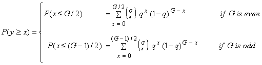 |
(3.1) |
Formally, if P(y >= x)= 1, the group 'can in principle stay alive', the group 'is able to maintain its existence'. However, as argued above, this can never be guaranteed unless q = 0. There always is a chance that the number of x-actors exceeds the number of y-actors, even if q is extremely small.
- 3.6
- This probability of group maintenance increases for even group sizes or for odd group sizes. The reason it does not increase from a group of even size to a group of odd size is the following. Suppose a group consists of an even number of actors. In the boundary situation of group maintenance, half the number of actors is in distress and each of them is helped by one and only one of the other half of the actors. Once one actor is added to this group, there will be no available helping partner in the boundary situation.
- 3.7
- Would we assume that all x-actors had information about which of the other actors are not in distress and also able to provide help (that is, which y-actors do not already provide help to another x-actor in this interval, or have helped another x-actor earlier this period), then, this probability (3.1) is the exact probability that the whole group can maintain its existence. The larger the group, the larger the chances of group maintenance. For q £0.2, chances of maintenance are beyond 0.99 as soon as G >= 14.
- 3.8
- Given our model assumptions however, this probability of group maintenance is smaller because actors do not have any information with regard to what other actors are in distress, let alone what other actors can provide help. As such, x-actors cannot be sure that the actors they ask for help, are y-actors that are able to provide help, and Equation (3.1) is an overestimation of the real probabilities. Appendix A illustrates the mathematical derivation of the probability of group maintenance given our assumptions. It is the probability that, within three successive intervals in a period, all x-actors are successful in finding a y-actor that can provide help. Since we have shown in the beginning of Section 3 that at least y should be larger than or equal to x, we condition on these situations. The result is the following:
- 3.9
- Let Pisuc(i) be the probability that, in the first interval of a period, i of the x-actors are successful in finding an helping partner among the y-actors. If x individuals are in distress, the number of successful x-individuals, i, can vary from 0 to x. It is self-evident that Pisuc(i) depends on both x and y:
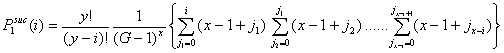 |
(3.2) |
- 3.10
- Let P2suc(i|i*) be the probability that i x-actors are successful in the second interval given that i* x-actors were successful in the first interval. Now, i can vary between 0 and x - i*.
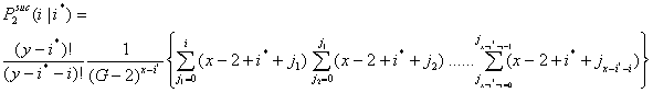 |
(3.3) |
- 3.11
- In a similar way, the probability for i successful actors in the third interval is given in Equation (3.4). Let
 be the probability that i x-actors are successful in the third interval given that i* x-actors were successful in the first and second interval.
 |
(3.4) |
- 3.12
- Given these probabilities of i x-actors being successful in each of the three intervals within a period, we compute the probability that all x-actors are successful within three intervals. The order in which these actors are successful can vary in different ways. For example, when three actors are in distress, there are ten different ways in which they all can find a helping partner. These possibilities are: (3 0 0), (0 3 0), (0 0 3), (2 1 0), (2 0 1), (1 2 0), (1 0 2), ( 0 1 2 ), (0 2 1), (1 1 1), where the first number within brackets indicates the number of successful actors in the first interval, the second number is the number of successful actors in the second interval, and the third number is the number of successful actors in the third interval. Each of these outcomes has a specific probability. Summed together, they determine the probability that three actors are successful. In Table 3.1 we show the probabilities that all x-actors are successful after three intervals in a period, for different values of x and G. We consider only those values of x and y for which y >= x. This shows that for group sizes smaller than G = 20, only when not more than 2 actors are distress, they will certainly find a helping partner within three intervals. Once there are more than 2 searching actors, there is always a probability, maybe very small, that not every actor succeeds in finding help. We see that this probability decreases as the group gets larger. When x = 3, and G = 6, the probability that not each of the three searching actors finds help is .536 ( 1 - .464), while it has decreased to .009 for G = 20.
|
| Table 3.1:Probability that all x actors in distress in a group of size G find a helping partner
|
|
|
|
|
|
|
| x |
|
|
|
|
|
| G | 0 | 1 | 2 | 3 | 4 | 5 | 6 | 7 | 8 | 9 | 10 |
|
|
|
|
|
|
|
|
|
|
|
|
| 1 | 1.00 |
|
|
|
|
|
|
|
|
|
|
| 2 | 1.00 | 1.00 |
|
|
|
|
|
|
|
|
|
| 3 | 1.00 | 1.00 |
|
|
|
|
|
|
|
|
|
| 4 | 1.00 | 1.00 | 1.00 |
|
|
|
|
|
|
|
|
| 5 | 1.00 | 1.00 | 1.00 |
|
|
|
|
|
|
|
|
| 6 | 1.00 | 1.00 | 1.00 | .464 |
|
|
|
|
|
|
|
| 7 | 1.00 | 1.00 | 1.00 | .693 |
|
|
|
|
|
|
|
| 8 | 1.00 | 1.00 | 1.00 | .810 | .208 |
|
|
|
|
|
|
| 9 | 1.00 | 1.00 | 1.00 | .875 | .405 |
|
|
|
|
|
|
| 10 | 1.00 | 1.00 | 1.00 | .914 | .555 | .091 |
|
|
|
|
|
| 11 | 1.00 | 1.00 | 1.00 | .938 | .663 | .218 |
|
|
|
|
|
| 12 | 1.00 | 1.00 | 1.00 | .954 | .740 | .343 | .039 |
|
|
|
|
| 13 | 1.00 | 1.00 | 1.00 | .965 | .797 | .453 | .111 |
|
|
|
|
| 14 | 1.00 | 1.00 | 1.00 | .973 | .838 | .545 | .198 | .017 |
|
|
|
| 15 | 1.00 | 1.00 | 1.00 | .978 | .870 | .621 | .288 | .054 |
|
|
|
| 16 | 1.00 | 1.00 | 1.00 | .982 | .893 | .682 | .373 | .108 | .007 |
|
|
| 17 | 1.00 | 1.00 | 1.00 | .986 | .912 | .731 | .450 | .172 | .026 |
|
|
| 18 | 1.00 | 1.00 | 1.00 | .988 | .926 | .772 | .518 | .240 | .057 | .003 |
|
| 19 | 1.00 | 1.00 | 1.00 | .990 | .938 | .805 | .578 | .308 | .099 | .012 |
|
| 20 | 1.00 | 1.00 | 1.00 | .991 | .947 | .832 | .629 | .372 | .148 | .029 | .001 |
|
- 3.13
- Going back to minimal group size, let us summarize briefly what the important aspects for this derivation are. First, in order for a group to be able to maintain existence, all actors that can get in distress, should be able to find a helping partner within three intervals of the same period. Since with a positive probability to get in distress, an exact assurance of group maintenance cannot be given, we had defined a minimum probability of .99 with which group maintenance can be guaranteed. Subsequently, as a minimal requirement for group maintenance, we have shown that the number of actors not in distress should be equal to or larger than the number of actors in distress (Equation (3.1)). A subsequent requirement is that all actors in distress are able to find a helping partner within three time intervals. Table 3.1 shows these probabilities for different values of x and G. Now, for group size G, we need to combine the probability that x actors are in distress, with the probability that these x actors all find a helping partner. This brings us to Tables 3.2, 3.3 and 3.4 for q = 0.05, q = 0.10, and q = 0.20 respectively. The final column in these tables is the sum of these probabilities for all different values of x, and gives us an estimate of the probability that a group of size G (in the corresponding row) can maintain existence. Be aware of the fact that the probabilities presented are all rounded numbers.
|
| Table 3.2:Probability that x actors are in distress and find help in group of size G, (q = 0.05) |
|
x
G |
| 0 | 1 | 2 | 3 | 4 | 5 | 6 | 7 | 8 | 9 | 10 | 11 | 12 | 13 | 14 | 15 | 16 | 17 | 18 | 19 | 20 |
|
| 0 |
| 1.0 |
|
|
|
|
|
|
|
|
|
|
|
|
|
|
|
|
|
|
|
| 1.0 |
| 1 |
| .95 | .00 |
|
|
|
|
|
|
|
|
|
|
|
|
|
|
|
|
|
|
| .95 |
| 2 |
| .90 | .10 | .00 |
|
|
|
|
|
|
|
|
|
|
|
|
|
|
|
|
|
| 1.0 |
| 3 |
| .86 | .14 | .00 | .00 |
|
|
|
|
|
|
|
|
|
|
|
|
|
|
|
|
| 1.0 |
| 4 |
| .81 | .17 | .01 | .00 | .00 |
|
|
|
|
|
|
|
|
|
|
|
|
|
|
|
| .99 |
| 5 |
| .77 | .20 | .02 | .00 | .00 | .00 |
|
|
|
|
|
|
|
|
|
|
|
|
|
|
| .99 |
| 6 |
| .74 | .23 | .03 | .00 | .00 | .00 | .00 |
|
|
|
|
|
|
|
|
|
|
|
|
|
| 1.0 |
| 7 |
| .70 | .26 | .04 | .00 | .00 | .00 | .00 | .00 |
|
|
|
|
|
|
|
|
|
|
|
|
| 1.0 |
| 8 |
| .66 | .28 | .05 | .01 | .00 | .00 | .00 | .00 | .00 |
|
|
|
|
|
|
|
|
|
|
|
| 1.0 |
| 9 |
| .63 | .30 | .06 | .01 | .00 | .00 | .00 | .00 | .00 | .00 |
|
|
|
|
|
|
|
|
|
|
| 1.0 |
| 10 |
| .60 | .32 | .07 | .01 | .00 | .00 | .00 | .00 | .00 | .00 | .00 |
|
|
|
|
|
|
|
|
|
| 1.0 |
| 11 |
| .57 | .33 | .09 | .01 | .00 | .00 | .00 | .00 | .00 | .00 | .00 | .00 |
|
|
|
|
|
|
|
|
| 1.0 |
| 12 |
| .54 | .34 | .10 | .02 | .00 | .00 | .00 | .00 | .00 | .00 | .00 | .00 | .00 |
|
|
|
|
|
|
|
| 1.0 |
| 13 |
| .51 | .35 | .11 | .02 | .00 | .00 | .00 | .00 | .00 | .00 | .00 | .00 | .00 | .00 |
|
|
|
|
|
|
| 1.0 |
| 14 |
| .49 | .36 | .12 | .03 | .00 | .00 | .00 | .00 | .00 | .00 | .00 | .00 | .00 | .00 | .00 |
|
|
|
|
|
| 1.0 |
| 15 |
| .46 | .37 | .13 | .03 | .00 | .00 | .00 | .00 | .00 | .00 | .00 | .00 | .00 | .00 | .00 | .00 |
|
|
|
|
| 1.0 |
| 16 |
| .44 | .37 | .14 | .04 | .01 | .00 | .00 | .00 | .00 | .00 | .00 | .00 | .00 | .00 | .00 | .00 | .00 |
|
|
|
| 1.0 |
| 17 |
| .42 | .37 | .16 | .04 | .01 | .00 | .00 | .00 | .00 | .00 | .00 | .00 | .00 | .00 | .00 | .00 | .00 | .00 |
|
|
| 1.0 |
| 18 |
| .40 | .38 | .17 | .05 | .01 | .00 | .00 | .00 | .00 | .00 | .00 | .00 | .00 | .00 | .00 | .00 | .00 | .00 | .00 |
|
| 1.0 |
| 19 |
| .38 | .38 | .18 | .05 | .01 | .00 | .00 | .00 | .00 | .00 | .00 | .00 | .00 | .00 | .00 | .00 | .00 | .00 | .00 | .00 |
| 1.0 |
| 20 |
| .36 | .38 | .19 | .06 | .01 | .00 | .00 | .00 | .00 | .00 | .00 | .00 | .00 | .00 | .00 | .00 | .00 | .00 | .00 | .00 | .00 | 1.0 |
|
|
| Table 3.3:Probability that x actors are in distress and find help in group of size G, (q = 0.10) |
|
x
G |
| 0 | 1 | 2 | 3 | 4 | 5 | 6 | 7 | 8 | 9 | 10 | 11 | 12 | 13 | 14 | 15 | 16 | 17 | 18 | 19 | 20 |
|
| 0 |
| 1.0 |
|
|
|
|
|
|
|
|
|
|
|
|
|
|
|
|
|
|
|
| 1.0 |
| 1 |
| .90 | .00 |
|
|
|
|
|
|
|
|
|
|
|
|
|
|
|
|
|
|
| .90 |
| 2 |
| .81 | .18 | .00 |
|
|
|
|
|
|
|
|
|
|
|
|
|
|
|
|
|
| .99 |
| 3 |
| .73 | .24 | .00 | .00 |
|
|
|
|
|
|
|
|
|
|
|
|
|
|
|
|
| .97 |
| 4 |
| .66 | .29 | .05 | .00 | .00 |
|
|
|
|
|
|
|
|
|
|
|
|
|
|
|
| 1.0 |
| 5 |
| .59 | .33 | .07 | .00 | .00 | .00 |
|
|
|
|
|
|
|
|
|
|
|
|
|
|
| .99 |
| 6 |
| .53 | .35 | .10 | .00 | .00 | .00 | .00 |
|
|
|
|
|
|
|
|
|
|
|
|
|
| .98 |
| 7 |
| .48 | .37 | .12 | .01 | .00 | .00 | .00 | .00 |
|
|
|
|
|
|
|
|
|
|
|
|
| .98 |
| 8 |
| .43 | .38 | .15 | .02 | .00 | .00 | .00 | .00 | .00 |
|
|
|
|
|
|
|
|
|
|
|
| .98 |
| 9 |
| .39 | .39 | .17 | .04 | .00 | .00 | .00 | .00 | .00 | .00 |
|
|
|
|
|
|
|
|
|
|
| .99 |
| 10 |
| .35 | .39 | .19 | .05 | .01 | .00 | .00 | .00 | .00 | .00 | .00 |
|
|
|
|
|
|
|
|
|
| .99 |
| 11 |
| .31 | .38 | .21 | .07 | .01 | .00 | .00 | .00 | .00 | .00 | .00 | .00 |
|
|
|
|
|
|
|
|
| .98 |
| 12 |
| .28 | .38 | .23 | .09 | .01 | .00 | .00 | .00 | .00 | .00 | .00 | .00 | .00 |
|
|
|
|
|
|
|
| .99 |
| 13 |
| .25 | .37 | .24 | .10 | .02 | .00 | .00 | .00 | .00 | .00 | .00 | .00 | .00 | .00 |
|
|
|
|
|
|
| .98 |
| 14 |
| .23 | .36 | .26 | .11 | .03 | .01 | .00 | .00 | .00 | .00 | .00 | .00 | .00 | .00 | .00 |
|
|
|
|
|
| 1.0 |
| 15 |
| .21 | .34 | .27 | .13 | .03 | .01 | .00 | .00 | .00 | .00 | .00 | .00 | .00 | .00 | .00 | .00 |
|
|
|
|
| .99 |
| 16 |
| .19 | .33 | .27 | .14 | .04 | .01 | .00 | .00 | .00 | .00 | .00 | .00 | .00 | .00 | .00 | .00 | .00 |
|
|
|
| .98 |
| 17 |
| .17 | .32 | .28 | .16 | .05 | .01 | .00 | .00 | .00 | .00 | .00 | .00 | .00 | .00 | .00 | .00 | .00 | .00 |
|
|
| .99 |
| 18 |
| .15 | .30 | .28 | .17 | .06 | .02 | .01 | .00 | .00 | .00 | .00 | .00 | .00 | .00 | .00 | .00 | .00 | .00 | .00 |
|
| .99 |
| 19 |
| .14 | .29 | .29 | .18 | .08 | .02 | .01 | .00 | .00 | .00 | .00 | .00 | .00 | .00 | .00 | .00 | .00 | .00 | .00 | .00 |
| 1.0 |
| 20 |
| .12 | .27 | .29 | .19 | .09 | .02 | .01 | .00 | .00 | .00 | .00 | .00 | .00 | .00 | .00 | .00 | .00 | .00 | .00 | .00 | .00 | .99 |
|
|
| Table 3.4:Probability that x actors are in distress and find help in group of size G, (q = 0.20) |
|
x
G |
| 0 | 1 | 2 | 3 | 4 | 5 | 6 | 7 | 8 | 9 | 10 | 11 | 12 | 13 | 14 | 15 | 16 | 17 | 18 | 19 | 20 |
|
| 0 |
| 1.0 |
|
|
|
|
|
|
|
|
|
|
|
|
|
|
|
|
|
|
|
| 1.0 |
| 1 |
| .80 | .00 |
|
|
|
|
|
|
|
|
|
|
|
|
|
|
|
|
|
|
| .80 |
| 2 |
| .64 | .32 | .00 |
|
|
|
|
|
|
|
|
|
|
|
|
|
|
|
|
|
| .96 |
| 3 |
| .51 | .38 | .00 | .00 |
|
|
|
|
|
|
|
|
|
|
|
|
|
|
|
|
| .89 |
| 4 |
| .41 | .41 | .15 | .00 | .00 |
|
|
|
|
|
|
|
|
|
|
|
|
|
|
|
| .87 |
| 5 |
| .33 | .41 | .20 | .00 | .00 | .00 |
|
|
|
|
|
|
|
|
|
|
|
|
|
|
| .94 |
| 6 |
| .26 | .39 | .25 | .04 | .00 | .00 | .00 |
|
|
|
|
|
|
|
|
|
|
|
|
|
| .94 |
| 7 |
| .21 | .37 | .28 | .08 | .00 | .00 | .00 | .00 |
|
|
|
|
|
|
|
|
|
|
|
|
| .94 |
| 8 |
| .17 | .34 | .29 | .12 | .01 | .00 | .00 | .00 | .00 |
|
|
|
|
|
|
|
|
|
|
|
| .93 |
| 9 |
| .13 | .30 | .30 | .16 | .03 | .00 | .00 | .00 | .00 | .00 |
|
|
|
|
|
|
|
|
|
|
| .92 |
| 10 |
| .11 | .27 | .30 | .18 | .05 | .00 | .00 | .00 | .00 | .00 | .00 |
|
|
|
|
|
|
|
|
|
| .91 |
| 11 |
| .09 | .24 | .30 | .21 | .07 | .01 | .00 | .00 | .00 | .00 | .00 | .00 |
|
|
|
|
|
|
|
|
| .92 |
| 12 |
| .07 | .21 | .28 | .23 | .10 | .02 | .00 | .00 | .00 | .00 | .00 | .00 | .00 |
|
|
|
|
|
|
|
| .91 |
| 13 |
| .05 | .18 | .27 | .24 | .12 | .03 | .00 | .00 | .00 | .00 | .00 | .00 | .00 | .00 |
|
|
|
|
|
|
| .89 |
| 14 |
| .04 | .15 | .25 | .24 | .14 | .05 | .01 | .00 | .00 | .00 | .00 | .00 | .00 | .00 | .00 |
|
|
|
|
|
| .88 |
| 15 |
| .04 | .13 | .23 | .24 | .17 | .06 | .01 | .00 | .00 | .00 | .00 | .00 | .00 | .00 | .00 | .00 |
|
|
|
|
| .88 |
| 16 |
| .03 | .11 | .21 | .25 | .18 | .08 | .02 | .00 | .00 | .00 | .00 | .00 | .00 | .00 | .00 | .00 | .00 |
|
|
|
| .88 |
| 17 |
| .02 | .10 | .19 | .24 | .19 | .10 | .03 | .01 | .00 | .00 | .00 | .00 | .00 | .00 | .00 | .00 | .00 | .00 |
|
|
| .88 |
| 18 |
| .02 | .08 | .17 | .23 | .20 | .12 | .04 | .01 | .00 | .00 | .00 | .00 | .00 | .00 | .00 | .00 | .00 | .00 | .00 |
|
| .87 |
| 19 |
| .01 | .07 | .15 | .22 | .21 | .13 | .06 | .01 | .00 | .00 | .00 | .00 | .00 | .00 | .00 | .00 | .00 | .00 | .00 | .00 |
| .86 |
| 20 |
| .01 | .06 | .14 | .21 | .21 | .14 | .07 | .02 | .00 | .00 | .00 | .00 | .00 | .00 | .00 | .00 | .00 | .00 | .00 | .00 | .00 | .86 |
|
- 3.14
- All values of x beyond the straight line correspond to y values that are smaller than x. As explained earlier, these are the situations in which not all of the x-actors can find y-actors. We see that for q = .05 and q = 0.10 the probabilities of group maintenance are .97 or higher for all different group sizes. Would we however assume that the probability of maintenance needs to exceed 0.99, for q = 0.05, group size needs at least to be 2. For q = 0.10, it is much more difficult to determine such a thing as a minimal group size because there is no monotone relationship between group size and probability of group maintenance. For q = 0.20 it seems that as group size increases beyond say, G = 10, chances of group maintenance actually decrease. The larger the group, the more actors can get in distress, and for these actors it is more difficult to find adequate helping partners, than for actors in smaller groups. So in this latter case, there is certainly no thing like a minimal group size, but maybe something like a maximal group size (or optimal, in between in a minimal and maximal value). In a larger group, two opposite things occur. On the one hand, more potential helping partners exist. On the other hand, the requirement that everyone should be able to stay alive is stronger. For now, it is difficult to exactly underpin the interaction effect between group size G and the probability to get in distress q. Our intuition does not bring us any further.
- 3.15
- Hence, it is difficult to define minimal group size in order to guarantee group maintenance. If there is anything, then it is an optimal instead of a minimal group size. However, our derivations show that for our values of q no clear solutions exist.[15] However, this does not mean that groups do not appear at all within the SEM.
The degree of segmentation
- 4.1
- We describe how we attempt to detect group structure in the networks of exchange relationships that emerge among the actors. We are interested in the structure of the network of surviving social actors only (asocial actors do not build any relationships). In the social network literature many different technical definitions of groups exist. Zeggelink et al. (1996) present an overview of most of these definitions together with a discussion of advantages and disadvantages. Since we do not want to restrict ourselves to just a particular kind of group definition (because it might exclude groups that we consider relevant, but just fall outside the scope of the definition), we turn to another network measure, the degree of segmentation or the segmentation index. The degree of segmentation is a summary measure of the distribution of distances in an undirected network (Baerveldt and Snijders 1994, Zeggelink 2000). A network is considered to be more segmented if the distances between nodes that are not directly connected, are on the average larger. This will always be true for a network in which a number of groups exist with relatively many relationships within the groups, and relatively few relationships between the groups.
- 4.2
- An important criterion for the segmentation index is thus the threshold where a distance becomes to be considered as large. In our case, a relationship between two actors exists if a mutual exchange has taken place. We do not distinguish the number of mutual exchanges, i.e. a relationship has the same meaning independent of the number of mutual exchanges. The distance between two actors in a network is defined as the length of the shortest path between them (e.g. the distance between two actors is 1 if there is a relationship between them; the distance is 2 if they have no direct exchange relationship, but both have an exchange relationship with at least one other common actor). As such, distances can be defined between all pairs of actors in a network (some of which may be infinite if there is neither a direct link nor an indirect path between the two).
- 4.3
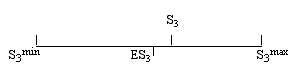
- The segmentation index now reflects a particular kind of dispersion of these distances namely the contrast between, on the one hand, the distances equal to 2, and on the other hand the 'long' distances. We define this threshold of 'long' at distance 3 for the following reasons. Distance 1 between a pair of actors implies an exchange relationship and that distance can be considered to be very close. Distance 2 between two actors implies a common exchange partner and may represent close. Analogously, distance 3 can be defined to be intermediate, and 4 or more is long. Subsequently, the exchange network is strongly segmented, and consequently shows at least some group formation, when most distances between the actors are either 1 or larger than or equal to 3. Distance 2 should not occur frequently. The corresponding segmentation index is called S3 .
- 4.4
- In notation: Let the resulting network consist of n social actors. The number of pairs in this network is equal to 1/2n(n-1). The density of the network is the number of realized exchange relationships between these pairs. Let now Db be the number of pairs at distance b. The fraction of pairs at distance b is
 |
(4.1) |
- 4.5
- It follows that F1 equals the density of the network (number of relationships divided buy the maximal possible number of relationships) and that F¥ is the fraction of pairs without any path between them. Qb is the fraction of pairs with distance larger than or equal to b.
| Qb = Fb + Fb + 1 +......+ F¥ = 1 - (F1 + F2 +......+ Fb - 1) |
(4.2) |
And our choice for the segmentation index S3 is now
 |
(4.3) |
- 4.6
- When the density is 1 (and consequently Q2 = 0), we define S3 = 0. The larger the value for S3 , the more segmented the network. S3 = 1 if the network is completely segmented: the network is divided into a number of disjoint cliques (in which density is maximal, and without any edges between the cliques). The higher the value of S3 , the longer (or non-existent) the 'social bridges' between unconnected nodes.
- 4.7
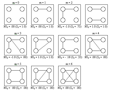
- Figure 4.1 shows, as an example, all possible networks with 5 actors, 4 relationships and different degrees of segmentation.
|
|
Figure 4.1. All graphs on 5 nodes with 4 edges
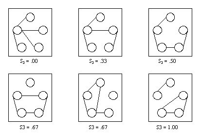
|
It illustrates that the degree of segmentation (even for an equal number of edges) may vary between S3 = .00 and S3 = 1.00. The more separated the nodes in the graph get, the higher the degree of segmentation, with its maximum for a complete separation into cliques.
- 4.8
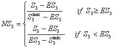
- Zeggelink (2000) developed a normalized version of the segmentation index that better controls for networks of different sizes and densities. The normalized segmentation index NS3 takes into account what the minimal S3 min, maximal S3 max, and expected value ES3 of the degree of segmentation is given the number of actors n and the number of relationships m. On the basis of these values, the normalized index is defined as:
 |
(4.4) |
- 4.9
- The workings of this normalization are illustrated below:
Where S3 could vary between 0 and 1, NS3 can now vary between the values -1 and 1. When S3 is larger than ES3 , NS3 is larger than 0, and closer to 1 as S3 gets closer to S3 max. A positive value of S3 means that the graph is more segmented than could be expected on the basis of a random distribution of the same number of edges among the same number of nodes. A value of NS3 smaller than 0, means that the graphs is less segmented than a random graph. NS3 = 1 means that the graphs is maximally segmented, NS3 = -1 means that the graph is minimally segmented.
Note that if S3 < 1, NS3 can still equal 1. This is the case if S3 = S3 max. If S3 = 1, NS3 = 0 or NS3 = 1. If NS3 = 1, this does not imply that S3 = 1. S3 can be smaller.
Simulation design
- 5.1
- We construct different types of initial situations. These situations differ only with respect to the total number of actors in the initial population, N, and the probability to get in distress, q. We consider N = 10 and N = 20 in combination with q = .05, q = .1, and q = .2. The number of social actors in the populations varies from 0 to 10 or 0 to 20 when N = 10 or N = 20 respectively. The total number of periods is 30. Since earlier results (De Vos and Zeggelink 1997) showed that the height of the costs of providing help had no significant effect on the end results, we combine the outcomes for all different values of these costs that we examined with a given value of q.[16] For every initial situation we do 50 simulations to obtain results on the number of surviving social and asocial actors and the network of exchange relationships. Since asocial actors do not establish any exchange relationships, we focus on the social actors and the networks they establish among each other. The size of such a network is the number of surviving social actors, n. It varies between 0 and N.
- 5.2
- The relationships within the 'social' network are defined on the basis of reciprocal exchanges. As soon as the number of mutual exchanges between two actors exceeds 1, a relationship between the two exists (the relationship is undirected).
- 5.3
- Density was defined in Section 4. If n = 0 or n = 1, density and the degree of segmentation are not defined because no pairs of actors exist. When n = 2, density d = 0 or d = 1, but the degree of segmentation still has no real meaning. We show the number of pairs (maximal number of relationships) in networks of size n = 0 to n = 20 in Table 5.1.
|
| Table 5.1:The number of pairs or the maximal number of relationships in networks of size n |
|
| n | maximal number of relationships
= n(n - 1) /2 | n | maximal number of relationships
= n(n - 1) /2 |
| | | | |
| 0 | 0 |
|
|
| 1 | 0 | 11 | 55 |
| 2 | 1 | 12 | 66 |
| 3 | 3 | 13 | 78 |
| 4 | 6 | 14 | 91 |
| 5 | 10 | 15 | 105 |
| 6 | 15 | 16 | 120 |
| 7 | 21 | 17 | 136 |
| 8 | 28 | 18 | 153 |
| 9 | 36 | 19 | 171 |
| 10 | 45 | 20 | 190 |
|
- 5.4
- We are mainly interested in the structure of the social 'social' network, and will examine the normalized degree of segmentation that emerges in these networks. In case the behavioral assumptions in the SEM indeed lead to group formation, we expect to find considerably higher values than 0 for the normalized degree of segmentation NS3 . The networks should substantively differ from random networks in the sense that they are much more segmented.
Results
- 6.1
- In order to see to what extent groups emerge, we take all simulated networks together that are of the same size n. We first make some remarks about the density of the networks that emerge, subsequently we turn to the more interesting degree of segmentation in the networks. Remember that n is the total number of social actors that survived, and that the density is the fraction of the actual number of realized exchange relationships (m), and the maximal possible number of relationships.
- 6.2
- If n = 2, density has no helpful meaning. The two actors are either connected or not, that is, the density is either 1 or 0. Results show that for q = 0.2, the two individuals are connected in 94% of the cases. For q = 0.1 and q = 0.05, these percentages are 76% and 53%. This already illustrates that with a decrease of q, the number of established relationships decreases too because actors have smaller probabilities to get in distress and as a result do not need to ask for help so often. Consequently, fewer relationships are established, and for some initial situations this leads to networks with zero density. This occurs for n = 3 and n = 4 with q = 0.1. For q = 0.05, even larger networks result that have zero density.
- 6.3
- Since networks of size n = 2 and n = 3 are not so relevant for the study of group formation (because no real groups can exist in such a small network), we start our analyses with networks of size n = 4. We first examine all theoretically possible networks and the corresponding values of the (normalized) degree of segmentation, presented in Figure 6.1.
|
|
Figure 6.1. All different networks of 4 actors
|
Only for two values of m, m = 2 or m = 3, non-zero values of NS3 exist. For m = 2, S3 = 0.75 or S3 = 1.00, corresponding by definition to NS3 = -1 and NS3 = 1, respectively. When m = 3, S3 = 0.00, S3 = 1.00, or S3 = 0.35, corresponding to NS3 = -1.00, NS3 = 1.00, and NS3 = -0.18, respectively.
- 6.4
- Hence, those two networks on four actors for which positive values of the normalized segmentation index exist, are the cases where NS3 is maximal, NS3 = 1. In all other networks, we see that NS3 = 0 or NS3 < 0. Thus we cannot expect to find a large normalized degree of segmentation at all with only a network of size n = 4. Moreover, speaking of group formation among only 4 actors is also difficult. Consequently the results for n = 4 are not so relevant and therefore only briefly reported here. Table B.1 in Appendix B shows detailed results for n = 4.
- 6.5
- With an initial population size of N = 10, 283 networks of size n = 4 emerged, when N = 20 we obtained 386 such networks. This difference is easily explained. For N = 20, these networks could have emerged from an initial proportion of 4 to 20 social actors. For N = 10, this could happen only for 4 to 10 social actors.[17] The number of relationships, m, in a network of size n = 4 can vary between m = 0 and m = 6. It increases when q increases as a result of the fact that an increase of q leads to a higher necessity for asking support, thereby leading to more exchange relationships in the networks. The normalized degree of segmentation NS3 of these networks shows no clear differences for different values of q and takes average values of NS3 = 0 or NS3 < 0. This confirms our earlier expectation that the networks of size n = 4 cannot be 'really segmented in groups'. They are on average less segmented than or equally segmented as could be expected on the basis of a random network on the same number of actors with the same number of relationships. Since the average normalized segmentation values for m = 2 and m = 3 are negative (Table B.1), the chain (m = 2, m = 3) network, or the star network (m = 3) emerged a little more often than the fully segmented networks consisting of 2 cliques of size 2 (m = 2), or one clique of size 3, and one clique of size 1 (m = 3) (Figure 6.1).
- 6.6
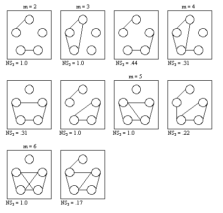
- Before we present the overall results for n = 5, we first examine what theoretically possible networks of five actors are that we would consider to consist of groups. Hence, which networks have such a degree of segmentation, that we conclude that groups are present. There are only few such networks when n = 5. All networks with a positive degree of normalized segmentation index are presented in Figure 6.2.
|
|
Figure 6.2. All networks of 5 actors with a positive normalized segmentation index
|
The degree of normalization has its own interpretation space. If we consider a network to be existing of very close(d) subgroups without any links between the groups, than only NS3 = 1 would suffice. However, for all networks of size n = 5 with a positive normalized segmentation index, it can be said that there has been at least some process of group formation. Beyond m = 6 relationships however, no positive normalized values of the segmentation index are possible (NS3 = 0 by definition).
- 6.7
- When we examine the results for n = 5, it appears that he average normalized degree of segmentation is positive only for m = 3 and m = 4. The corresponding networks in Figure 6.2 appear relatively more often than the more chain- and star-like networks with m = 3 and m = 4 relationships. With more exchange relationships, that is with a higher density, networks are either less or equally segmented in comparison with random networks. Similar reasons can be given for these results as for n = 4, because it is difficult to speak of any 'real group formation' within in a network of only 5 actors.
- 6.8
- When the surviving social population consists of n = 6 actors, some degree of group formation occurs again only for the smaller values of relationships, m = 2 to m = 5.
- 6.9
- In Tables 6.1a and 6.1b we present a summarized overview of results for all different values of network size. The rows in these tables correspond to the number of established exchange relationships m. In Table 6.1a, the main columns correspond to the different sizes n (n = 4 to n = 10) of the social end population that emerged. The subcolumns of N = 10 and N = 20 represent whether that population emerged with an initial population of 10 or 20 actors respectively. In Table 6.1b results are shown for values of n beyond n = 10, so all of these end populations could emerge only for initial population sizes of N = 20. Bold values of the normalized degree of segmentation indicate positive values, that is, the degree of segmentation is higher than expected on the basis of random networks.
|
| Table 6.1a: Normalized degree of segmentation for different social populations n = 4 to n = 10 |
|
| n |
| 4 | 5 | 6 | 7 | 8 | 9 | 10 |
| N |
| m |
| 10 | 20 | 10 | 0 | 10 | 20 | 10 | 20 | 10 | 20 | 10 | 20 | 10 | 20 |
|
|
|
|
|
|
|
|
|
|
|
|
|
|
|
|
| 2 |
| -0.02 | -0.17 | -0.05 | 0.28 | 0.32 | 0.19 | 0.65 | 0.46 | 0.72 | 0.50 | 0.48 | 0.52 | 0.55 | 0.65 |
| 3 |
| -0.19 | -0.13 | 0.17 | 0.13 | 0.31 | 0.29 | 0.30 | 0.29 | 0.54 | 0.38 | 0.20 | 0.40 | 0.28 | 0.23 |
| 4 |
| 0.00 | 0.00 | 0.00 | 0.00 | 0.17 | 0.17 | 0.19 | 0.22 | 0.19 | 0.34 | 0.24 | 0.32 | 0.26 | 0.34 |
| 5 |
| 0.00 | 0.00 | -0.31 | -0.37 | 0.01 | 0.15 | 0.09 | 0.18 | 0.24 | 0.22 | 0.35 | 0.28 | 0.25 | 0.30 |
| 6 |
| 0.00 |
| -0.17 | -0.87 | -0.06 | -0.10 | 0.04 | 0.08 | 0.21 | 0.17 | 0.19 | 0.23 | 0.26 | 0.32 |
| 7 |
|
|
| 0.00 |
| -0.28 | -0.29 | 0.00 | 0.02 | 0.08 | 0.11 | 0.17 | 0.17 | 0.13 | 0.16 |
| 8 |
|
|
| 0.00 |
| -0.10 | 0.17 | -0.19 | -0.07 | 0.01 | 0.06 | 0.08 | 0.09 | 0.15 | 0.18 |
| 9 |
|
|
|
|
| -1.00 | -1.00 | -0.10 | -0.09 | 0.03 | -0.03 | 0.05 | 0.08 | 0.12 | 0.12 |
| 10 |
|
|
|
|
| -1.00 |
| -0.36 | -0.39 | -0.17 | -0.17 | -0.02 | 0.01 | 0.06 | 0.07 |
| 11 |
|
|
|
|
| 0.00 |
| -1.00 |
| -0.27 | 0.10 | 0.10 | 0.06 | 0.06 | 0.05 |
| 12 |
|
|
|
|
|
|
|
|
| -0.06 | -0.22 | -0.05 | -0.08 | 0.00 | 0.06 |
| 13 |
|
|
|
|
|
|
|
|
| 0.04 | -0.61 | -0.20 |
| -0.01 | -0.03 |
| 14 |
|
|
|
|
|
|
| -1.00 |
|
|
| -0.33 |
| -0.21 | -0.06 |
| 15 |
|
|
|
|
|
|
|
|
|
|
| -0.09 |
| -0.12 | 0.11 |
| 16 |
|
|
|
|
|
|
|
|
|
|
|
|
| 0.09 | -0.54 |
| 17 |
|
|
|
|
|
|
|
|
|
|
|
|
| -0.43 |
|
| .. |
|
|
|
|
|
|
|
|
|
|
|
|
|
| |
|
|
| Table 6.1b: Normalized degree of segmentation for different social populations n =11 to n = 20 |
|
|
|
|
|
|
| n |
|
|
|
|
|
| m |
| 11 | 12 | 13 | 14 | 15 | 16 | 17 | 18 | 19 | 20 |
|
|
|
|
|
|
|
|
|
|
|
|
| 2 |
|
| -0.33 | 0.00 | 0.00 | 0.00 | 0.00 | 0.00 |
|
|
|
| 3 |
|
| 0.38 | 0.67 | 0.33 | 1.00 | 1.00 | 0.00 | 0.00 | -0.13 |
|
| 4 |
| 0.75 | 0.34 | 0.35 | 0.42 | 0.78 | 0.83 | 0.75 | 0.83 | 0.87 | 1.00 |
| 5 |
| 0.52 | 0.30 | 0.41 | 0.21 | 0.42 | 0.71 | 0.61 | 0.52 | 0.62 | 0.83 |
| 6 |
| 0.28 | 0.35 | 0.30 | 0.19 | 0.23 | 0.31 | 0.24 | 0.39 | 0.40 | 0.60 |
| 7 |
| 0.14 | 0.34 | 0.39 | 0.36 | 0.25 | 0.33 | 0.25 | 0.28 | 0.23 | 0.35 |
| 8 |
| 0.29 | 0.15 | 0.16 | 0.22 | 0.21 | 0.34 | 0.25 | 0.34 | 0.25 | 0.43 |
| 9 |
| 0.20 | 0.16 | 0.23 | 0.16 | 0.23 | 0.29 | 0.25 | 0.31 | 0.22 | 0.35 |
| 10 |
| 0.19 | 0.13 | 0.24 | 0.21 | 0.34 | 0.27 | 0.22 | 0.28 | 0.21 | 0.25 |
| 11 |
| 0.14 | 0.09 | 0.21 | 0.19 | 0.23 | 0.26 | 0.31 | 0.21 | 0.26 | 0.25 |
| 12 |
| 0.15 | 0.12 | 0.11 | 0.19 | 0.17 | 0.24 | 0.30 | 0.28 | 0.30 | 0.39 |
| 13 |
| 0.03 | 0.09 | 0.14 | 0.12 | 0.14 | 0.22 | 0.16 | 0.18 | 0.21 | 0.21 |
| 14 |
| 0.01 | 0.09 | 0.08 | 0.13 | 0.10 | 0.14 | 0.14 | 0.19 | 0.22 | 0.23 |
| 15 |
| 0.02 | 0.02 | 0.08 | 0.15 | 0.10 | 0.17 | 0.09 | 0.20 | 0.23 | 0.22 |
| 16 |
| -0.07 | 0.01 | 0.08 | 0.06 | 0.18 | 0.16 | 0.16 | 0.16 | 0.12 | 0.27 |
| 17 |
|
| -0.10 | 0.02 | 0.08 | 0.06 | 0.08 | 0.10 | 0.15 | 0.14 | 0.20 |
| 18 |
|
| -0.29 | -0.01 | 0.06 | 0.02 | 0.13 | 0.14 | 0.14 | 0.20 | 0.15 |
| 19 |
|
|
| 0.00 | 0.03 | 0.08 | 0.14 | 0.10 | 0.15 | 0.15 | 0.16 |
| 20 |
|
|
|
| 0.08 | 0.05 | 0.06 | 0.11 | 0.11 | 0.14 | 0.22 |
| 21 |
|
|
|
| -0.05 | 0.02 | 0.03 | 0.11 | 0.08 | 0.04 | 0.13 |
| 22 |
|
|
|
| 0.00 | 0.00 | 0.07 | 0.11 | 0.09 | 0.08 | 0.00 |
| 23 |
|
|
| - 0.12 |
| 0.05 | 0.02 | 0.03 | 0.08 | 0.17 | 0.06 |
| 24 |
|
|
|
|
| -0.02 | 0.09 | 0.06 | 0.06 | 0.02 | 0.08 |
| 25 |
|
|
|
|
|
| 0.00 | -0.04 | 0.03 | 0.13 | 0.08 |
| 26 |
|
|
|
|
|
| -0.04 | 0.22 | 0.00 | 0.01 | 0.18 |
| 27 |
|
|
|
|
|
|
|
| 0.03 | 0.03 |
|
| 28 |
|
|
|
|
|
|
|
|
|
|
|
| 29 |
|
|
|
|
|
|
|
|
|
| 0.15 |
| 30 |
|
|
|
|
|
|
|
|
|
|
|
| 31 |
|
|
|
|
|
|
|
|
|
| 0.06 |
| 32 |
|
|
|
|
|
|
|
|
|
| 0.10 |
| .. |
|
|
|
|
|
|
|
|
|
| |
|
The normalized segmentation decreases as the number of relationships that emerged increases. The index is highest for small values of m and decreases to negative values as the number of relationships get higher. For larger population sizes, negative normalized segmentation values do not always occur. In the vast majority the index remains positive.
- 6.10
- A positive normalized segmentation index means that the network is more segmented than could be expected on the basis of a random network with the same number of relationships, but does not necessarily mean that subgroups are present. Would subgroups be clearly present, than the normalized segmentation index would need to be close to 1. Although the determination of the existence of subgroups is free for interpretation (Are links between groups allowable or not? Should all actors within a group be connected to each other? How many actors should be connected? How many outside connections are allowed? See also our discussion at the beginning of Section 4), it seems that the higher segmentation indices (NS3 > 0.50) indicate 'real' subgroup presence. This means that our results show that there is not yet a clear general tendency towards group formation, but to a certain extent there is segmentation. Since this effect disappears when many exchange relationships exist, it is partly a side effect of the number of exchange relationships established, and thereby of the probability to get in distress. The latter determines the number of exchange relationships that emerges. Since we already concluded in Section 3 that is difficult to arrive at something like optimal group size, it is not so surprising that we do not find any clear group formation by now either.
- 6.11
- Nevertheless, the question remains why networks emerge at all with a degree of segmentation that is higher than for random networks. The main reason seems to be that when different actors get in distress, they need help from different actors, and thereby construct a potential for constructing exchange relationships in different parts of the population or network. Moreover, the priority given to actors with whom one has exchanged most often is also an important element that leads to segmentation. Not reported results on social actors who do not necessarily 'prefer-old-helping-partners' show a much smaller degree of segmentation. When social actors did not have this 'prefer-old-helping-partners' trait, networks emerged that look much more like random networks. Actually these networks had a degree of segmentation that was on the average smaller than could be expected on the basis of random networks.[18]
- 6.12
- Given the current assumptions in the SEM, the element that pushes segmentation back however, is that in a pair of individuals help cannot be given twice in the same direction successively.
Conclusion and discussion
- 7.1
- We have argued that the Social Evolution Model (SEM) provides not only a potential explanation of the emergence of cooperation, but at the same time of the observed degree of group living among humans. Previously we had investigated the viability of social (reciprocal altruistic) and asocial (cheating) strategies of giving and requesting support. We found that actors with social strategies take over a small population if their proportion is not too small and if conditions are harsh, that is, if receiving support is of considerable importance for survival. In larger populations and if their proportions are not too small, they are able to prevent a take-over by the asocial strategies. Given these earlier findings, we studied here to what extent the SEM already provides a potential solution towards the problem of the emergence of group living.
- 7.2
- The basic dynamics within the model SEM were as follows: At the beginning of a so-called period, an actor has a certain probability to get in distress (survival and/or reproduction is at stake). In the complete set of actors, a number of them actually gets in distress, others do not. Those who are in distress cannot survive if they do not receive support from other actors. Help can be received, only if asked for. Thus, those who are in distress will ask other actors for help. By receiving or providing support one's own survival/reproduction probabilities increase or decrease respectively. The latter occurs because, by the provision of support, resources that could have been used for one's own survival/ reproduction are used up. Actors differ in the strategies they use for asking and providing support. These strategies, social or asocial, are the main model components and partly determined by the cognitive capacities of the actors. Within a certain period, an actor has a limited number of possibilities to ask others for help. Right now, we assume that an actor can ask only one other actor per time, and an actor has only three such chances within a period. An actor cannot provide help, if he is in distress himself. Moreover, an actor can only support one other actor within a single period. The probability to get in distress in the next period increases when providing help in this period.
- 7.3
- On the basis of mutual help provisions, a network of exchange relations between the actors in the group develops. The strength of these relations, depends on the number of help exchanges that has taken place between these individuals. This results in a population of which some actors have died, and others have not. Among the latter, in particular among the social actors, an exchange network has developed. It is the structure of this network that we examined in order to see whether some kind of group formation has taken place.
- 7.4
- Unfortunately, but not totally surprising regarding the model assumptions as they are, group formation does not really occur. Simulation results show that there is not a clear tendency towards group formation, but to a certain extent there is segmentation. This effect however disappears when many exchange relationships exist. So it is partly a side effect of the number of exchange relationships established, and thereby of the probability to get in distress. The latter determines the number of exchange relationships that emerges. Thus we could also conclude that under the assumptions of the SEM as it exists now, some considerable amount of segmentation (or group formation) only occurs when the probability to get in distress is small.
- 7.5
- However, some preliminary results related to work in De Vos et al. (2000) show that complete segmentation (!) - probably through pairs of actors- occurs once the social actors apply the so-called commitment strategy. With regard to helping behavior an actor applying this commitment strategy is prepared to help unconditionally another actor who ever provided help, if that actor is the only one who asks for help. If he has to select a receiver of his help from several candidates from whom he received help in the past, he then selects the one who provided help most often, irrespective of the number of times he returned his help. With respect to asking behavior the only difference with the social strategy reported here concerns the case when there are two or more others he helped in the past. He selects the one from whom he received help or from whom he received help most often. If there are two or more from whom he received help most often, he asks the one that is most in his debt. These very preliminary results may suggest that the social strategy reported here may need to be modified into the direction of the commitment strategy.
- 7.6
- Since we had also concluded that is difficult to derive an optimal group size, given the assumptions in the SEM, results are not very disappointing. In particular because we have seen that the networks that emerge have a degree of segmentation that is higher than for random networks. The main reason seems to be that when different actors get in distress, they need help from different actors, and thereby construct a potential for constructing exchange relationships in different parts of the population or network. This brings us to the expectation that more segmentation may be found when larger populations are considered.
- 7.7
- Moreover, the priority given to actors with whom one has exchanged most often is also an important element that leads to segmentation. This effect will be increased as soon as we allow for indirect reciprocity as an option to pay one's debts to another actor that has more often provided than received help from you. And, as mentioned above, this effect will also be increased as soon as the social strategy contains more elements of the commitment strategy.
- 7.8
- Other interesting and relevant future activities may concern the combination of the results in this paper with those of the earlier papers in which we were purely interested in survival probabilities of the different strategies. A very interesting thing to do would be to examine the degree of segmentation over time, and to see whether there is an effect on survival probabilities. As such, we would not only examine the effects of cooperation on the degree of group formation but also the other way around.
- 7.9
- Moreover, and this holds for any kind of simulation research, it would be important to see how sensitive the SEM is for the parameter choices and strategy definitions that we have taken. So far, we have considered those values that we thought were theoretically most appropriate for our problem definition.
Appendix A
-
We derive the probability that, within three successive intervals in a period, all x-actors are successful in finding a y-actor that can provide help.[19] Since we have shown in the beginning of Section 3 that at least y should be larger than or equal to x, we condition on this situation.
Before we derive the desired probability we first present an example of the choice process in the first interval.
Assume the total number of actors in the population is six (G = 6). Let the number of actors in distress be three (x = 3). The number of y-actors thus also equals three (y = 3). All x-actors will choose among all other actors. Since every actor x has (G-1) = 5 alternatives, the total number of possible choices is (G-1)x = 53 = 125. All these possibilities are given in Table A.1. The columns (1) and (1a) give the number of the possibility. The columns (2) and (2a), (3) and (3a), (4) and (4a) present the choice of the first, second, and third x-actor respectively. The columns (5) and (5a) show the number of successful actors. From these 125 possibilities, 8 choice combinations (1, 2, 6, 7, 11, 12, 16, 17) lead to no successes. In that case, all x-actors choose on of the other x-actors. 57 choice combinations lead to 1 success. In that case, only one of the x-actors chooses a y-actor, or two or three x-actors choose one and the same y-actor. 54 choice combinations lead to 2 successes and only 6 choice combinations (70, 74, 90, 98, 114, 118) lead to three successes. In the latter case, all three x-actors choose a unique y-actor. As such, the probability of no success is 8/125 = .064, the probability of 1 successful actor is 57/125 = .456, the probability of two successes is 54/125 = .432, and the probability of three successes is 6/125 = .048.
|
| Table A.1: All potential outcomes of choices of 3 x-actors in a group of 6 actors, first interval |
|
(1)
out-come | (2)
choice x1 | (3)
choice x2 | (4)
choice x3 | (5)
#
successful actors | (1)
out-come | (2a)
choice x1 | (3a)
choice x2 | (4a)
choice x3 | (5a)
#
successful actors |
|
|
|
|
|
|
|
|
|
|
| 1 | x2 | x1 | x1 | 0 | 36 | x3 | y1 | x1 | 1 |
| 2 | x2 | x1 | x2 | 0 | 37 | x3 | y1 | x2 | 1 |
| 3 | x2 | x1 | y1 | 1 | 38 | x3 | y1 | y1 | 1 |
| 4 | x2 | x1 | y2 | 1 | 39 | x3 | y1 | y2 | 2 |
| 5 | x2 | x1 | y3 | 1 | 40 | x3 | y1 | y3 | 2 |
| 6 | x2 | x3 | x1 | 0 | 41 | x3 | y2 | x1 | 1 |
| 7 | x2 | x3 | x2 | 0 | 42 | x3 | y2 | x2 | 1 |
| 8 | x2 | x3 | y1 | 1 | 43 | x3 | y2 | y1 | 2 |
| 9 | x2 | x3 | y2 | 1 | 44 | x3 | y2 | y2 | 1 |
| 10 | x2 | x3 | y3 | 1 | 45 | x3 | y2 | y3 | 2 |
| 11 | x3 | x1 | x1 | 0 | 46 | x3 | y3 | x1 | 1 |
| 12 | x3 | x1 | x2 | 0 | 47 | x3 | y3 | x2 | 1 |
| 13 | x3 | x1 | y1 | 1 | 48 | x3 | y3 | y1 | 2 |
| 14 | x3 | x1 | y2 | 1 | 49 | x3 | y3 | y2 | 2 |
| 15 | x3 | x1 | y3 | 1 | 50 | x3 | y3 | y3 | 1 |
| 16 | x3 | x3 | x1 | 0 | 51 | y1 | x1 | x1 | 1 |
| 17 | x3 | x3 | x2 | 0 | 52 | y1 | x1 | x2 | 1 |
| 18 | x3 | x3 | y1 | 1 | 53 | y1 | x1 | y1 | 1 |
| 19 | x3 | x3 | y2 | 1 | 54 | y1 | x1 | y2 | 2 |
| 20 | x3 | x3 | y3 | 1 | 55 | y1 | x1 | y3 | 2 |
| 21 | x2 | y1 | x1 | 1 | 56 | y1 | x3 | x1 | 1 |
| 22 | x2 | y1 | x2 | 1 | 57 | y1 | x3 | x2 | 1 |
| 23 | x2 | y1 | y1 | 1 | 58 | y1 | x3 | y1 | 1 |
| 24 | x2 | y1 | y2 | 2 | 59 | y1 | x3 | y2 | 2 |
| 25 | x2 | y1 | y3 | 2 | 60 | y1 | x3 | y3 | 2 |
| 26 | x2 | y2 | x1 | 1 | 61 | y1 | y1 | x1 | 1 |
| 27 | x2 | y2 | x2 | 1 | 62 | y1 | y1 | x2 | 1 |
| 28 | x2 | y2 | y1 | 2 | 63 | y1 | y1 | y1 | 1 |
| 29 | x2 | y2 | y2 | 1 | 64 | y1 | y1 | y2 | 2 |
| 30 | x2 | y2 | y3 | 2 | 65 | y1 | y1 | y3 | 2 |
| 31 | x2 | y3 | x1 | 1 | 66 | y1 | y2 | x1 | 2 |
| 32 | x2 | y3 | x2 | 1 | 67 | y1 | y2 | x2 | 2 |
| 33 | x2 | y3 | y1 | 2 | 68 | y1 | y2 | y1 | 2 |
| 34 | x2 | y3 | y2 | 2 | 69 | y1 | y2 | y2 | 2 |
| 35 | x2 | y3 | y3 | 1 | 70 | y1 | y2 | y3 | 3 |
|
|
| Table A.1 (continued): All potential outcomes of choices of 3 x-actors in a group of 6 actors |
|
(1)
out-come | (2)
choice x1 | (3)
choice x2 | (4)
choice x3 | (5)
#
successful actors | (1)
out-come | (2a)
choice x1 | (3a)
choice x2 | (4a)
choice x3 | (5a)
#
successful actors |
|
|
|
|
|
|
|
|
|
|
| 71 | y1 | y3 | x1 | 2 | 101 | y3 | x1 | x1 | 1 |
| 72 | y1 | y3 | x2 | 2 | 102 | y3 | x1 | x2 | 1 |
| 73 | y1 | y3 | y1 | 2 | 103 | y3 | x1 | y1 | 2 |
| 74 | y1 | y3 | y2 | 3 | 104 | y3 | x1 | y2 | 2 |
| 75 | y1 | y3 | y3 | 2 | 105 | y3 | x1 | y3 | 1 |
| 76 | y2 | x1 | x1 | 1 | 106 | y3 | x3 | x1 | 1 |
| 77 | y2 | x1 | x2 | 1 | 107 | y3 | x3 | x2 | 1 |
| 78 | y2 | x1 | y1 | 2 | 108 | y3 | x3 | y1 | 2 |
| 79 | y2 | x1 | y2 | 1 | 109 | y3 | x3 | y2 | 2 |
| 80 | y2 | x1 | y3 | 2 | 110 | y3 | x3 | y3 | 1 |
| 81 | y2 | x3 | x1 | 1 | 111 | y3 | y1 | x1 | 2 |
| 82 | y2 | x3 | x2 | 1 | 112 | y3 | y1 | x2 | 2 |
| 83 | y2 | x3 | y1 | 2 | 113 | y3 | y1 | y1 | 2 |
| 84 | y2 | x3 | y2 | 1 | 114 | y3 | y1 | y2 | 3 |
| 85 | y2 | x3 | y3 | 2 | 115 | y3 | y1 | y3 | 2 |
| 86 | y2 | y1 | x1 | 2 | 116 | y3 | y2 | x1 | 2 |
| 87 | y2 | y1 | x2 | 2 | 117 | y3 | y2 | x2 | 2 |
| 88 | y2 | y1 | y1 | 2 | 118 | y3 | y2 | y1 | 3 |
| 89 | y2 | y1 | y2 | 2 | 119 | y3 | y2 | y2 | 2 |
| 90 | y2 | y1 | y3 | 3 | 120 | y3 | y2 | y3 | 2 |
| 91 | y2 | y2 | x1 | 1 | 121 | y3 | y3 | x1 | 1 |
| 92 | y2 | y2 | x2 | 1 | 122 | y3 | y3 | x2 | 1 |
| 93 | y2 | y2 | y1 | 2 | 123 | y3 | y3 | y1 | 2 |
| 94 | y2 | y2 | y2 | 1 | 124 | y3 | y3 | y2 | 2 |
| 95 | y2 | y2 | y3 | 2 | 125 | y3 | y3 | y3 | 1 |
| 96 | y2 | y3 | x1 | 2 |
|
|
|
|
|
| 97 | y2 | y3 | x2 | 2 |
|
|
|
|
|
| 98 | y2 | y3 | y1 | 3 |
|
|
|
|
|
| 99 | y2 | y3 | y2 | 2 |
|
|
|
|
|
| 100 | y2 | y3 | y3 | 2 |
|
|
|
| |
|
Now let p1suc(i) be the probability that, in the first interval of a period, i of the x-actors are successful in finding an helping partner among the y-actors. If x individuals are in distress, the number of successful x-individuals, i, can vary from 0 to x. It is self-evident that Pisuc(i) depends on x and y:
 |
(A.1) |
This probability in (A.1) is derived and defined as the number of successful outcomes divided by the total number of ways ((G-1)x) in which x searching actors can choose among all other (G-1) actors. The first fraction in (A.1) is the number of possible ways in which i of the x actors in distress can be successful. This means that it represents the number of distinct ways that these i x-actors can choose i different y-actors: y such actors exist who can provide help. Each actor in distress chooses, in order to be successful, one single and unique y-actor. Suppose that i = 1, this means that the chosen y-actor (no matter how many x-actors choose this y-actor) can be either of the y y-actors (y = y!/ (y - 1)!). Therefore the term within brackets is multiplied by the fraction y!/(y - i)!
The product of sums within brackets represents the ways in which the choices of the (x-i) unsuccessful actors can be arranged over the other (G-1-i) actors.[20] Since these actors are unsuccessful, they choose either from the other actors in distress (x-1 others), or they choose one of the y-actors (i are 'occupied') that has been asked by a successful x-actor already. The term within the first summation sign relates to the first unsuccessful actor, and based on his choice, choices of the other actors are 'restricted' in such a way that double patterns are avoided. Within these summations jk controls for the number of y-actors that has been chosen already. It should be noted that there is a new second sum for every step of the iterator of the first sum, and so forth.
If i = 0 for example, none of the actors in distress is successful. This means that all x actors choose among themselves (and for the product within brackets only terms with j1 = j2 = ...jx = 0 will occur). If i = 1, all (x-1) unsuccessful actors choose either the same y that the successful actor chooses, or they choose one of the other x actors. This returns in the summations dependent on whether the first not successful actor chooses that y-actor (j1 = 1) or not.
Returning to our example, we fill in x = 3, y = 3 and G = 6 and obtain:
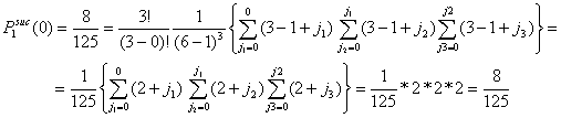
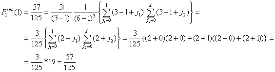
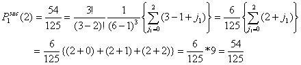
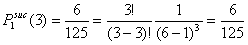
All actors that are not successful in the first interval however have two additional chances to find a helping y-actor. Equation (A.1) thus needs to be extended for those cases in which less than x actors are successful. What happened when i is smaller than x? This means that x-i actors either asked another x-actor for help or asked one of the i y-actors that was simultaneously (in the same first interval) asked by another x-actor (who got preferred randomly). Every unsuccessful x-actor knows that he should not ask that actor again (actors not in distress can help only one actor in a period). The unsuccessful x-actors however still do not know who the actors in distress, or the actors not in distress are.[21]
In general, this translates for the second interval only for a change in the parameter values of (A.1). Let P2suc(i|i*) be the probability that i x-actors are successful in the second interval given that i* x-actors were successful in the first interval. Now, i can vary between 0 and x - i*. Going from Equation (A.1) to Equation (A.2), the number of searching actors changes from x to x-i*, the number of available helping y-actors changes from y to y - i*, and the number of possibilities changes from (G-1)x to (G-2)x-i* because every unsuccessful x-actor will not return to that actor he asked for help in the first time interval. All x - i* actors can still ask all other x-actors, and also all i* y-actors that cannot provide help anymore.
 |
(A.2) |
In a similar way, the probability for i successful actors in the third interval can be derived, resulting in Equation (A.3). Let P3suc(i|i*) be the probability that i x-actors are successful in the third interval given that a total of i* x-actors were successful in the first and second interval.
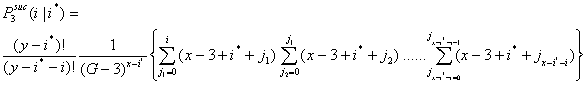 |
(A.3) |
Appendix B
-
We show detailed result for networks of size n = 4 in Table B.1.
|
| Table B1: S3 for networks of 4 actors (n = 4) with different densities |
|
|
|
|
|
| a | N = 10 |
|
|
|
|
| (1) | (2) | (3) | (4) | (5) | (6) | (7) | (8) | (9) | (10) | (11) |
| m | den |
|
|
| q |
|
|
|
|
|
|
| 0.20 |
| 0.10 |
| 0.05 |
|
| tot |
|
|
|
S3 |
# |
S3 |
# |
S3 |
# |
S3 |
NS3 |
# |
|
|
|
|
|
|
|
|
|
|
|
| 0 | 0.00 |
|
| 1.00 (.00) | 2 | 1.00 (.00) | 22 | 1.00 (.00) | 0.00 (.00)° | 24 |
| 1 | 0.17 | 1.00 (.00) | 4 | 1.00 (.00) | 14 | 1.00 (.00) | 47 | 1.00 (.00) | 0.00 (.00) | 65 |
| 2 | 0.33 | 0.95 (.10) | 15 | 0.87 (.13) | 36 | 0.83 (.12) | 29 | 0.87 (.13) | -0.02 (1.01) | 80 |
| 3 | 0.50 | 0.37 (.19) | 27 | 0.28 (.13) | 30 | 0.44 (.27) | 6 | 0.33 (.18) | -0.19 (.36) | 63 |
| 4 | 0.67 | 0.00 (.00) | 25 | 0.00 (.00) | 8 | 0.00 ( -- ) | 1 | 0.00 (.00) | 0.00 (.00) | 34 |
| 5 | 0.83 | 0.00 (.00) | 12 | 0.00 (.00) | 2 |
|
| 0.00 (.00) | 0.00 (.00) | 14 |
| 6 | 1.00 | 0.00 (.00) | 3 |
|
|
|
| 0.00 (.00) | 0.00 (.00) | 3 |
|
|
|
|
|
|
|
|
|
|
|
|
|
|
|
|
|
|
| 0.64 (.40) | -0.05 (.56) | 283 |
|
|
|
|
| b | N = 20 |
|
|
|
|
|
|
|
|
|
|
|
|
|
|
|
| 0 | 0.00 |
|
| 1.00 (.00) | 2 | 1.00 (.00) | 27 | 1.00 (.00) | 0.00 (.00) | 29 |
| 1 | 0.17 | 1.00 (.00) | 6 | 1.00 (.00) | 29 | 1.00 (.00) | 66 | 1.00 (.00) | 0.00 (.00) | 101 |
| 2 | 0.33 | 0.88 (.13) | 38 | 0.87 (.13) | 54 | 0.81 (.11) | 34 | 0.85 (.12) | -0.17 (.99) | 126 |
| 3 | 0.50 | 0.29 (.11) | 48 | 0.44 (.28) | 42 | 0.67 (.47) | 2 | 0.37 (.23) | -0.13 (.44) | 92 |
| 4 | 0.67 | 0.00 (.00) | 29 | 0.00 (.00) | 3 |
|
| 0.00 (.00) | 0.00 (.00) | 32 |
| 5 | 0.83 | 0.00 (.00) | 6 |
|
|
|
| 0.00 (.00) | 0.00 (.00) | 6 |
| 6 | 1.00 |
|
|
|
|
|
|
|
|
|
|
|
|
|
|
|
|
|
|
|
|
|
|
|
|
|
|
|
| 0.70 (.36) | -0.09 (.61) | 386 |
|
° Italic values of the normalized index represent that no other values of NS3 are possible, so nothing can be concluded from these networks.
Table B.1 shows the results for n = 4, N = 10 (a) and N = 20 (b) respectively. In column (1) we present the number of realized exchange relationships that can vary between 0 and the maximal possible number (see Table 5.1). In column (2) we present the corresponding density of the network. Columns (3) and (4), (5) and (6), and (7) and (8) show the average degree of segmentation and standard deviation within brackets and the number of cases (networks) on which the average is computed, for q = 0.20, q = 0.10, and q = 0.05, respectively. Column (9) gives the average and standard deviation of S3 over all values of q together. Column (10) presents the corresponding normalized segmentation index NS3 , and column (11) presents the number of cases on which the values in columns (10) and (11) are based.
Acknowledgements
-
The research of Evelien Zeggelink has been made possible by a fellowship from the Royal Netherlands Academy of Arts and Sciences. We thank the anonymous reviewers for their very useful comments on an earlier version of this manuscript.
Notes
-
1 Humans have lived in closed or semi-closed groups of hunter-gatherers larger than the conjugal family. Only until very recently, relatively speaking in terms of the history of human mankind, the only relations humans had, were more or less durable and personal and with kin as well as non-kin, although not always face-to-face from day to day. Different estimations exist of the sizes of these groups. One recent estimation is based on the relation between group size and relative volume of the neocortex of primates, and gives a group size of 150 (Dunbar 1993).
2In Zeggelink (1998) such a potential explanation was given for the emergence of groups in the context of friendship relations, that is, within the larger scope of friendship networks.
3Kranton (1996) allows for the unlimited potential choice for new partners (cooperation) after an initially specified matching of partners. On the basis of certain assumptions, actors can always find a new partner if they terminate an existing relationship. Cooperation can however still be sustained if actors monotonically increase the level of cooperation within a relationship. With this strategy it is always better to continue in a current relationship than to 'cheat' and start again with a new partner. Her analyses suggest, but do not show right away, that when information is costly, establishing communities within which cooperation can be sustained must involve cost barriers to entry. Consequently a population can become segmented into different groups.
4Hence, the proportion of social strategies, the harshness of conditions (determining the probability of actors to get in distress), and the size of the initial population are the main factors that determine the viability of the social strategy.
5Boorman and Levitt (1980) make the implicit assumption that endogamous social units are already present in the initial stage of their model. The problem of explaining the emergence of a local concentration of sociality remains unsolved. A similar assumption exists in the work of Boyd and Richerson (1985) who start with the ethnic group as a basis. Other studies incorporate likewise assumptions (Axelrod 1984, Boyd and Richerson 1988 , Reeve 1998).
6Related to group living on the basis of reciprocal altruism is the so-called communal orientation of the group members. A communal orientation means a concern for each other's and one's own welfare. You benefit each other in response to need and in order to demonstrate concern. Receipt of a benefit does not create a specific debt or obligation to return a comparable benefit soon afterward. Neither does it alter the general obligation both of you have to be responsive to each other's needs (Mills and Clark 1982).
7 This is neither to say that such a situation is easy to define, nor that humans ever actually lived in these circumstances. However, if we say a socially unstructured population, it is important to be precise about what the absence of structure means. We mean that the only social relations assumed to exist initially are kinship relations. The elementary units in our model are basically conjugal or extended families. At the outset, these units have no mutual social relationships. For simplicity's sake, we call these elementary actors 'individuals' or 'actors', because they are the only acting units in our model.
"Scratch" does not mean the complete absence of cooperation. An appropriate way to formulate the problem is to start with a population in which the individuals are organized in kinship groups and with kin-directed altruism concentrated exclusively within the units. This population could be interpreted as an abstraction of a Pleistocene social organization of hunters and gatherers, with all non-kinship-based-cooperation removed. The units then resemble so-called minimal bands that consist of 'several families of consanguine and/or affinal relatives who, at least during part of the year, share a common settlement and participate in a given range of cultural activities'. Then, the kind of cooperation to be explained is the tendency of a minimal band 'to participate in a larger social network in order to enhance its chance of biological and cultural survival', this larger network being called the maximal band (Wobst 1974).
8Whenever we refer to an individual by 'he', we also mean to refer to the female form.
9 Since it concerns actors with equal differences, this implies that this is the same actor for which the number of times support provided is highest.
10Since a social actor will never provide help to another actor twice in a row, without having been helped by that other actor in between, the difference number of times help given and received will either be equal to -1, 0, or 1 for every other actor.
11For reasons mentioned in the previous footnote, an asocial actor will never receive help from a social actor once he has already received help from that actor in a previous time period. However, an asocial actor does not have this knowledge. Would we assume that he had this knowledge, it would make more sense for an asocial actor to just distinguish other actors in those who have helped and those who have not.
12The choice of this value is certainly discussible (see Dawkins 1976)
13We do not take into account here that an actor will not provide help to the same actor twice in a row (in different periods) if that other actor has not provided help in return in between.
14We do not consider group size beyond G = 20 because we have simulation results only for initial population sizes up to 20.
15 Things would look different if we would allow for group growth, for instance as a result of 'birth-' and immigration' processes. That would be possible, if we would consider generations one after the other.
16For q = 0.2, this combines the results for costs of help being equal to c = 0.1, c = 0.05, and c = 0.025. For q = 0.1, this combines the results for c = 0.05, c = 0.025, and c = 0.0125. For q = 0.05, this combines the results for c = 0.025, c = 0.0125, and c = 0.00625. For every value of q, the total number of cases is 1650.
17This is therefore the general tendency, also for larger networks of social actors: Looking at a network of a certain size, it appeared more frequently for N = 20 than for N = 10. However, for N = 20 the percentages of networks with low density occur relatively more frequently than the networks with high density.
18 Other not reported results, related to the work in De Vos et al. (2000), show that segmentation increases to the extreme end once social actors apply the so-called commitment strategy.
19Actually, we would also have to take into account that reciprocity comes into play. We would need to know what the probability is to ask another actor, that is not in distress, for help, when we know that an actor asks those that have been helped by him before. This becomes too cumbersome. It would, among other things, mean taking into account that an actor's probability to get in distress increases in the period following the period he has helped another actor.
20If x = i, all actors in distress are successful and the whole term within braces. This probability definition is completely based on the lack of knowledge of all actors, and asks for a new definition in case more information would be available to the actors. This would for example imply higher probabilities for the same number of successes if only actors would be able to know which actors are in distress and which are not.
21Actors in distress that succeed in the first interval, and as a result get help, cannot provide help in this period. Only at the beginning of the next period they are defined to be no longer in distress.
References
-
AXELROD R (1984) The evolution of cooperation. New York: Basic Books.
AXELROD R and Hamilton W D (1981) The evolution of cooperation in biological systems. Science 211. pp. 1390-1396.
BAERVELDT C and Snijders T A B (1994) Influences on and from the segmentation of networks: hypotheses and tests. Social Networks. pp. 213-232.
BOORMAN S A and Levitt P R (1980) The genetics of altruism. New York: Academic Press.
BOYD R and Richerson P J (1985) Culture and the Evolutionary Process. Chicago: University of Chicago Press.
BOYD R and Richerson P J (1988) The evolution of reciprocity in sizeable groups. Journal of Theoretical Biology 132. pp. 337-356.
BREWER M B and Miller N (1996) Intergroup relations. Buckingham: Open University Press.
BREWER M B and Kramer R M (1986) Choice behavior in social dilemmas: effects of social identity, group size, and decision framing. Journal of Personality and Social Psychology 50. pp. 543-549.
BROWN J S, Sanderson M J and Michod R E (1982) Evolution of social behavior by reciprocation. Journal of Theoretical Biology 99. pp. 319-339.
CAMPBELL B (1979) Ecological factors and social organization in human evolution. In Bernstein I S and Smith E O (Eds.), Ecology and human origins: ecological influences on social organization. New York: Garland STPM Press.
COOPER B and Wallace C (1998) Evolution, partnerships and cooperation. Journal of Theoretical Biology 195. pp. 315-329.
DAWKINS R (1976) The Selfish Gene. Oxford: Oxford University Press
DE VOS H and Zeggelink E P H (1994) The emergence of reciprocal altruism and group-living: an object oriented simulation model of human social evolution. Social Science Information 33. pp. 493-517.
DE VOS H and Zeggelink E P H (1997) Reciprocal altruism in human social evolution: the viability of reciprocal altruism with a preference for 'old-helping-partners'. Evolution and Human Behavior 18. pp. 261-278.
DE VOS H, Smaniotto R and Elsas D A (2000) Reciprocal altruism under conditions of partner selection. Under review.
DUNBAR, R I M (1993) Coevolution of neocortical size, group size, and human language. Behavioral and Brain Sciences 16. pp. 681-694.
DUGATKIN L A and Wilson D S (1991) ROVER: A strategy for exploiting cooperators in patchy environments. The American Naturalist 138. pp. 687-701.
ERICKSON, B. (1988) "The relational basis of attitudes". In B. Wellman, and S. Berkowiz (Eds.) Social Structures: A network approach. Cambridge: Cambridge University Press.
FLACHE A. and Hegselmann R (1999) Altruism vs. self-interest in social support. Computer simulations of cooperation and partners election in social support networks. Advances in Group Processes 16. pp. 61-97.
FREEMAN L C (1992) The sociological concept of 'group': an empirical test of two models. American Journal of Sociology 98. pp. 152-166.
GALANTER M (1978) The 'relief-effect': A sociobiological model for neurotic distress and large- group therapy. American Journal of Psychiatry 135. pp. 588-591.
HOMANS, G. (1950) The human group. New York: Harcourt Brace.
KNAUFT B M (1991) Violence and sociality in human evolution. Current Anthropology 32. pp. 391-409
KRAMER R M, and Brewer M B (1984) Effects of group identity on resource use in a simulated commons dilemma. Journal of Personality and Social Psychology 46. pp. 1044-1057.
KRAMER R M, and Brewer M B (1986) Social group identity and the emergence of cooperation in resource conservation dilemmas. In Wilke H A M, Messick D M and Rutte G C (Eds.), Experimental social dilemmas. Frankfurt: Peter Lang.
KRANTON R E (1996) The formation of cooperative relationships. Journal of Law, Economics, and Organization 12. pp. 214-223.
KURLAND J A and Beckerman S J (1985) Optimal foraging and hominid evolution: Labor and reciprocity. American Anthropologist 87. pp. -93
MACY M W and Skvoretz J(1998) The evolution of trust and cooperation between strangers: a computational model. American Sociological Review 63. pp. 638-660.
MILLS J and Clark M S (1982) Exchange and communal relationships. In Wheeler L (Ed.), Review of personality and social psychology, vol. 3. Beverly Hills: Sage.
MULLEN, B. and G. Goethals (1987) Theories of group behavior. New York: Springer-Verlag.
NETTLE D and Dunbar R I (1997) Social markers and the evolution of reciprocal exchange. Current Anthropology 38. pp. 93-99.
NOWAK M A and May R M (1992) Evolutionary games and spatial chaos. Nature 359. pp. 826-829.
NOWAK M A, Bonhoefer S, and May R M (1994a) Spatial games and the maintenance of cooperation. Proceedings of the National Academy of Sciences 91. pp. 4877-4881.
NOWAK M A, Bonhoefer S and May R M (1994b) More spatial games. International Journal of Bifurcation Chaos 4. pp. 33-56.
REEVE H R (1998) Acting for the good of others: kinship and reciprocity with some new twists. In Crawford C C and Krebs D L (Eds.) Handbook of Evolutionary Psychology. Ideas, Issues, and Applications. Mahwah, N.J.: Erlbaum.
ROOK, K.S. (1987) "Social support versus companionship: effects on life stress, loneliness, and evaluations by others". Journal of Personality and Social Psychology 52: 1132-1147.
SHAW M. (1981) Group dynamics: the psychology of small group behavior. New York: McGraw-Hill.
SCHUESSLER R. (1989) Exit threats and cooperation under anonymity. Journal of conflict resolution 33. pp. 728-749.
STANLEY E A, Ashlock D and Smucker M D (1995) Iterated Prisoner's Dilemma with choice and refusal of partners: evolutionary results. Lecture Notes in Computer Science 929. pp. 495-502.
STEVENS, A. and J. Price (1997) Evolutionary Psychiatry. London:
Routledge.
TAJFEL, H. and J. Turner (1986) "The social identity theory of intergroup-behavior". In S. Worchel and W. Austin (Eds.) Psychology of intergroup relations. Chicago: Nelson-Hall Publishers.
TRINKAUS E (1989) The upper Pleistocene transition. In Trinkaus E (Ed.) The emergence of modern humans: Biocultural adaptation in the later Pleistocene. Cambridge: Cambridge University Press.
TRIVERS R (1971) The evolution of reciprocal altruism. Quarterly Review of Biology 46. pp. 35-56.
VANBERG V J and Congleton R D (1992) Rationality, morality, and exit. American political science review 86. pp. 418-431.
WILSON D S and Dugatkin L A (1997) Group selection and assortative interactions. The American Naturalist 149. pp. 336-351.
WINTERHALDER B. (1986) Diet choice, risk, and food sharing in a stochastic environment. Journal of Anthropological Archaeology 5. pp. 369-392.
WOBST H M. (1974) Boundary conditions for Paleolithic social systems: a simulation approach. American Antiquity 39. pp. 147-178.
YAMAGISHI T, Hayashi N and Jin N (1994) Prisoner's dilemma networks: selection strategy versus action strategy. In Schulz U, Albers W and Mueller U (Eds.) Social dilemmas and cooperation. New York: Springer Verlag.
ZEGGELINK E P H, Stokman F N, and Van De Bunt G G (1996) The emergence of groups in the evolution of friendship networks. Journal of Mathematical Sociology 21. pp. 29-55.
ZEGGELINK, E.P.H. (1998) "Group formation in friendship networks". In P. Doreian and T. Fararo (Eds.) The problem of solidarity: theories and models. Amsterdam: Gordon and Breach Publishers.
ZEGGELINK E P H. (2000) The degree of segmentation reconsidered. Paper to be presented at the Fifth International Conference on Social Science Methodology in Cologne, Germany, October 3-6, 2000.
 Return to Contents of this issue
© Copyright Journal of Artificial Societies and Social Simulation, 1999