Anne Di Piazza and Erik Pearthree (1999)
Journal of Artificial Societies and Social Simulation vol. 2, no. 3, <https://www.jasss.org/2/3/4.html>
To cite articles published in the Journal of Artificial Societies and Social Simulation, please reference the above information and include paragraph numbers if necessary
Received: 8-Jun-99 Accepted: 27-Aug-99 Published: 31-Oct-99
![]()
 Abstract

|
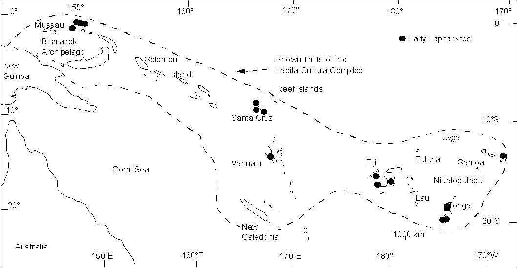
| Map 1: Distribution of the earliest Lapita sites in Oceania (after Kirch, 1997:54) |
As presently defined on the basis of archaeological surveys, the Lapita world began in the Bismarck Archipelago in the west, and extended through the island arcs of the Solomons and Vanuatu, down to New Caledonia in the south. It also reached across the 850 km wide ocean gap between the Santa Cruz Islands and Fiji, to encompass the Fiji, Lau, Tonga, and Samoa archipelagoes, as well as several smaller islands... A temporal cline extending from the Bismarck Archipelago south to New Caledonia and east to the Fiji-Tonga-Samoa region marks the path of the Lapita diaspora, a phase of population expansion occurring in no less than three and no more than five centuries. The total straight-line geographic distance involved is about 4,500 km, so that the 'average' rate of dispersal or population movement was on the order of 9-15 km per year. Naturally, in an island world dispersal would not have taken place 1 km at a time, but rather in 'jumps' of varying distance. It may be more insightful, therefore, to think of this dispersal in terms of human generations. If each successive generation had a reproduction span of about 20 years, the Lapita diaspora required somewhere between 15 and 25 generations to accomplish. This suggests that, again on 'average', each successive generation moved eastwards or southwards somewhere between 180 and 300 km.
| Table 1:Today's age structure and growth rate for several archipelagos in Oceania (Quid, 1998:896 and web site http://www.census.gov ) | |||
Archipelago | Growth rate (%) | Children <15 years (%) | Adults 15 years (%) |
| Fiji | 1.5 | 38 | 62 |
| Marshalls | 4.1 | 51 | 49 |
| FSM | - | 44 | 56 |
| New Caledonia | 1.9 | 31 | 69 |
| French Polynesia | - | 36 | 64 |
| Solomons | 3.7 | 47 | 53 |
| Samoa | 1.8 | 41 | 59 |
| Vanuatu | 2.8 | 44 | 56 |
| Initial Population | Migration rate (%) | Growth rate (%) | |
|---|---|---|---|
| -x- | 50 | 5 | 1 |
| -o- | 200 | 20 | 4 to 2 |
| - - | 5200 | 20 | 2 |

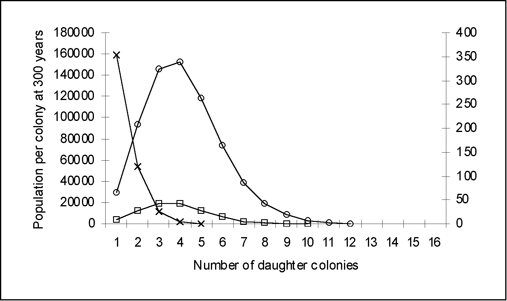
| Iteration 1 -x- | Iteration 2 -o- | Iteration 3 - - | |
|---|---|---|---|
| Colony 0 | 354 | 29,605 | 3,582 |
| Daughter Colony 1 | 120 | 93,374 | 12,230 |
| Daughter Colony 2 | 25 | 146,154 | 19,389 |
| Daughter Colony 3 | 4 | 152,383 | 18,916 |
| Daughter Colony 4 | 0 | 118,114 | 12,687 |
| Daughter Colony 5 | 0 | 73,601 | 6,189 |
| Daughter Colony 6 | 0 | 39,126 | 2,264 |
| Daughter Colony 7 | 0 | 18,645 | 631 |
| Daughter Colony 8 | 0 | 8,424 | 135 |
| Daughter Colony 9 | 0 | 3018 | 22 |
| Daughter Colony 10 | 0 | 559 | 3 |
| Daughter Colony 11 | 0 | 58 | 0 |
| Daughter Colony 12 | 0 | 4 | 0 |
| Daughter Colony 13 | 0 | 0 | 0 |
| Total Population | 989 | 683,065 | 76,047 |
Figure 1: Population distribution per colony at the end of the Lapita expansion (300 years). Using the widest range of parameter values, with colonies created every 20 years and with a cut-off of 10 people, the number of daughter colonies varies from 3 to 11 (in bold). On the graph, note that two different scales have been used. Iteration 1 has to be read with the right vertical axis. Iteration 2 and 3 have to be read with the left vertical axis.

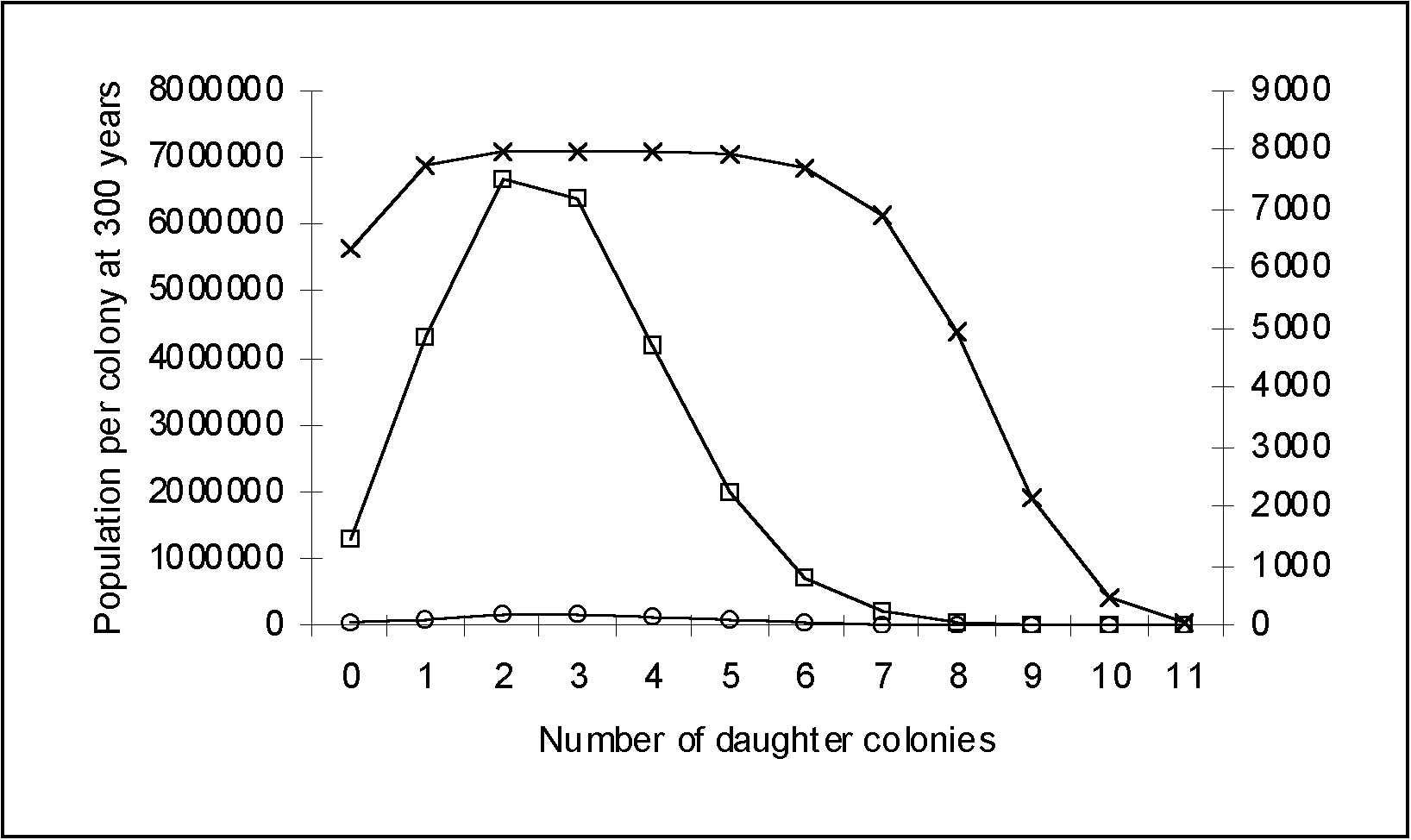
| - - Population per colony with a growth rate of 4% | -o- Population per colony with a growth rate of 4% to 2% | -x- Population per colony with a growth rate of 4% to 0% | |
|---|---|---|---|
| Colony 0 | 1,295,612 | 29,605 | 6,328 |
| Daughter Colony 1 | 4,318,707 | 93,374 | 7,738 |
| Daughter Colony 2 | 6,683,714 | 146,154 | 7,956 |
| Daughter Colony 3 | 6,365,442 | 152,383 | 7,985 |
| Daughter Colony 4 | 4,167,849 | 118,114 | 7,973 |
| Daughter Colony 5 | 1,984,690 | 73,601 | 7,911 |
| Daughter Colony 6 | 708,818 | 39,126 | 7,682 |
| Daughter Colony 7 | 192,876 | 18,645 | 6,918 |
| Daughter Colony 8 | 40,182 | 8,424 | 4,949 |
| Daughter Colony 9 | 6,378 | 3,018 | 2,138 |
| Daughter Colony 10 | 759 | 559 | 463 |
| Daughter Colony 11 | 66 | 58 | 53 |
| Daughter Colony 12 | 4 | 4 | 4 |
| Daughter Colony 13 | 0 | 0 | 0 |
| Total population | 25,765,097 | 683,065 | 68,095 |
Figure 2: Population distribution and number of daughter colonies founded at 300 years using an initial population of 200, a migration rate of 20% and variable growth rates. Daughter colonies are created every 20 years (one generation). Even though the number of daughter colonies are the same (11) for all runs, the total population is very different. On the graph, note that two different scales have been used. The 4% and the 4% to 2% growth rate curves have to be read with the left vertical axis. The 4% to 0% growth rate curve has to be read with the right vertical axis. On the table, note that the population in column 2 is far greater than today's population. This iteration has to be rejected.

|
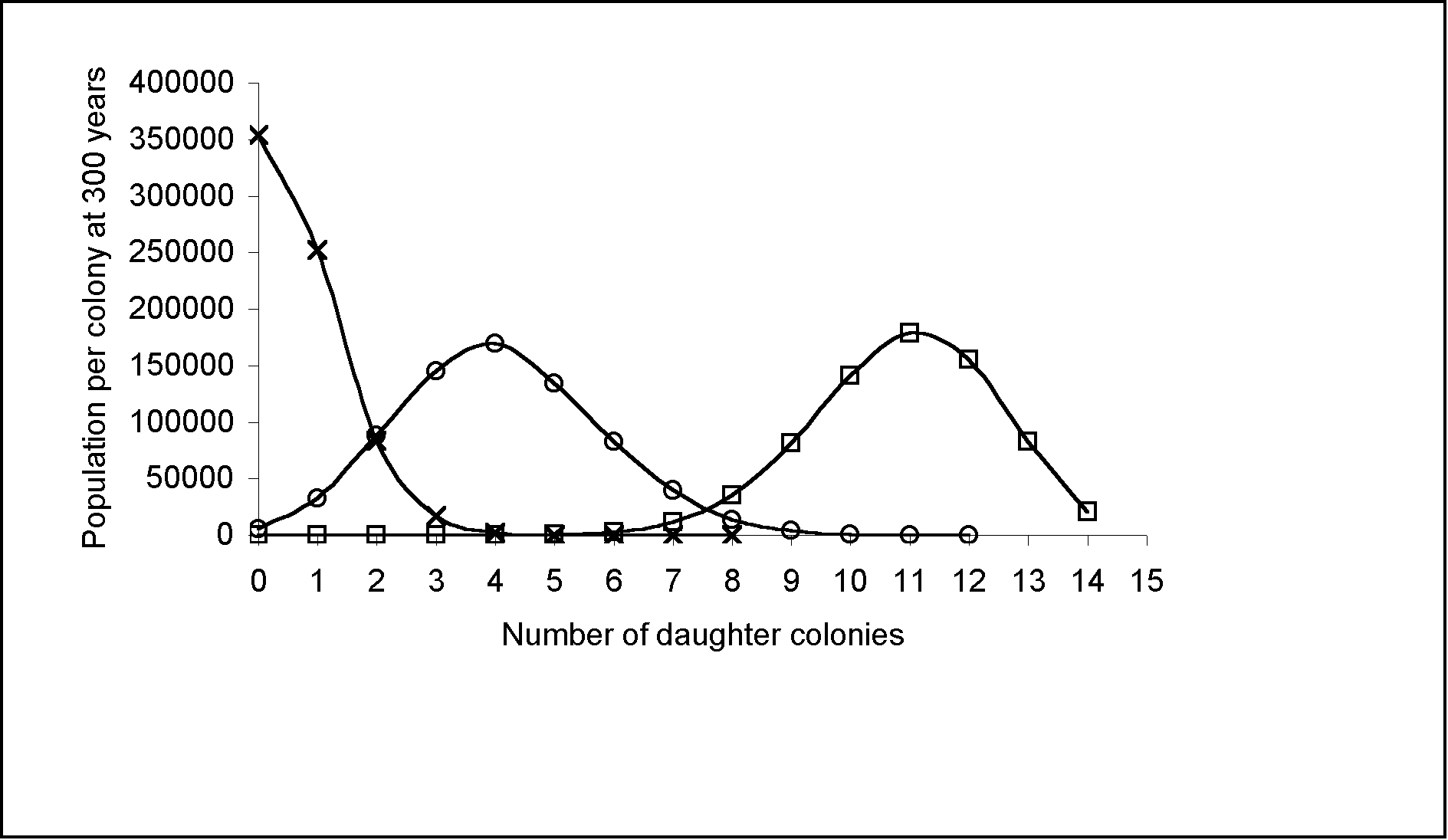
Figure 3: Population distribution per colony at 300 years using an initial population of 100, a growth rate of 3% and variable migration rates. Daughter colonies are created every 20 years (one generation). At a migration rate of 5%, 95% of the population remains with the original colony. Therefore more people are concentrated in the west, near the Bismarck Archipelago. At a higher migration rate, the population concentration shifts eastward. A 30% migration rate or more, leads to a depopulation of the Bismarck Archipelago.
| Table 2: Inventory of the earliest Lapita archaeological sites (after Kirch, 1997:263-276) | |
| Archipelago | Early Lapita Site |
|---|---|
| Bismarck/Mussau | Talepakemalai Etapakengaroasa Epakapaka Apalo |
| Reef/Santa Cruz | Nenumbo Nanggu Malu & Bianga Mepala |
| Vanuatu | Malo |
| Fiji | Natunuku Yanuca Naigani |
| Tonga | Moala Pe'a Tongoleleka Faleloa |
| Samoa | To'aga |
 Notes
Notes2 The earliest and farthest west that archaeologists have so far been able to trace the Lapita trail is the Bismarck Archipelago.
3 The best example known to the author is the British colonial scheme from the southern Gilberts to the Phoenix Islands (Kiribati) in 1937-1938, where a maximum of 15% of the population of one island (Beru) migrated. However, the average migration rate of the other 7 islands was about 3% (Maude, 1938:20; Maude 1968). Even 15% was only attained once and then only with coercion.
4 Out of a population of 100, 29 are adult males (potential sailors). For a 10% migration rate, there are 10 migrants, 5 of who are sailors. This represents 17% of the adult men out of the original group (5 x100/29).
5 1.5 million includes only native populations, excluding colonial immigrants.
6 STELLA software is available from High Performance Systems, Inc, 45 Lyme Road, Hanover NH 03755, USA.
7 The maximum number of daughter colonies is obtained with a growth rate of 4% decreasing to 2% or of 4% decreasing to 0% when the population reaches 8000 people and a migration rate of 20%.
KIRCH P.V. 1990 La colonisation du Pacifique. La Recherche no.225, vol.21:1226-1235.
KIRCH P.V. 1997 The Lapita Peoples. Ancestors of the Oceanic World. Blackwell Publishers, Oxford.
MAUDE H.E. 1938 Colonization of the Phoenix Islands by the surplus population of the Gilbert and Ellice Islands. Confidential Report, Government Press, Suva.
MAUDE H.E 1968 Of Islands and Men. Studies in Pacific History. Oxford University Press, Melbourne.
QUID 1998 Tout sur tout et un peu plus que tout, Laffont, Paris.
PAWLEY A. and GREEN R.C. 1973 Dating the dispersal of the Oceanic languages. Oceanic Linguistics 12:1-67.
SPRIGGS M. 1997 The Island Melanesians. The Peoples of the South-East Asia and the Pacific. Blackwell Publishers, Oxford.
SUTTON D.G. and MOLLOY M. A. 1989 Deconstructing Pacific palaeodemography : a critique of density dependent causality. Archaeology in Oceania, 24:31-36. TERRELL J. 1986 Prehistory in the Pacific Islands. Cambridge University Press, Cambridge.
THORNE A. and RAYMOND R. 1989 Man on the Rim. The peopling of the Pacific. Angus and Robertson Publishers, Auckland.
Colony0(t) = Colony0(t - dt) + (Croiss_Esp0 - Migra01) * dt
INIT Colony0 = 200
INFLOWS: Croiss_Esp0 = Colony0*Tx_Croiss
OUTFLOWS: Migra01 = if time=20 then Colony0*Tx_Migr else if time=40 then Colony0*Tx_Migr else if time=60 then Colony0*Tx_Migr else if time=80 then Colony0*Tx_Migr else if time=100 then Colony0*Tx_Migr else if time=120 then Colony0*Tx_Migr else if time=140 then Colony0*Tx_Migr else if time=160 then Colony0*Tx_Migr else if time=180 then Colony0*Tx_Migr else if time = 200 then Colony0*Tx_Migr else if time =220 then Colony0*Tx_Migr else if time=240 then Colony0*Tx_Migr else if time= 260 then Colony0*Tx_Migr else if time=280 then Colony0*Tx_Migr else 0
Colony1(t) = Colony1(t - dt) + (Migra01 + Croiss_Esp1 - Migra12) * dt
INIT Colony1 = 0
INFLOWS: Migra01 = if time=20 then Colony0*Tx_Migr else if time=40 then Colony0*Tx_Migr else if time=60 then Colony0*Tx_Migr else if time=80 then Colony0*Tx_Migr else if time=100 then Colony0*Tx_Migr else if time=120 then Colony0*Tx_Migr else if time=140 then Colony0*Tx_Migr else if time=160 then Colony0*Tx_Migr else if time=180 then Colony0*Tx_Migr else if time = 200 then Colony0*Tx_Migr else if time =220 then Colony0*Tx_Migr else if time=240 then Colony0*Tx_Migr else if time= 260 then Colony0*Tx_Migr else if time=280 then Colony0*Tx_Migr else 0
Croiss_Esp1 = Colony1*Tx_Croiss
OUTFLOWS: Migra12 = if time=40 then Colony1*Tx_Migr else if time=60 then Colony1 *Tx_Migr else if time = 80 then Colony1*Tx_Migr else if time=100 then Colony1*Tx_Migr else if time=120 then Colony1*Tx_Migr else if time=140 then Colony1*Tx_Migr else if time=160 then Colony1*Tx_Migr else if time=180 then Colony1*Tx_Migr else if time=200 then Colony1*Tx_Migr else if time=220 then Colony1*Tx_Migr else if time=240 then Colony1*Tx_Migr else if time=260 then Colony1*Tx_Migr else if time=280 then Colony1*Tx_Migr else 0
Colony10(t) = Colony10(t - dt) + (Migr910 + Croiss_esp10 - Migr1011) * dt
INIT Colony10 = 0
INFLOWS: Migr910 = if time = 200 then Colony9*Tx_Migr else if time = 220 then Colony9*Tx_Migr else if time = 240 then Colony9*Tx_Migr else if time = 260 then Colony9*Tx_Migr else if time = 280 then Colony9*Tx_Migr else 0
Croiss_esp10 = Colony10*Tx_Croiss
OUTFLOWS: Migr1011 = if time = 220 then Colony10*Tx_Migr else if time = 240 then Colony10*Tx_Migr else if time = 260 then Colony10*Tx_Migr else if time = 280 then Colony10*Tx_Migr else 0
Colony11(t) = Colony11(t - dt) + (Migr1011 + Croissesp11 - Migr1112) * dt
INIT Colony11 = 0
INFLOWS: Migr1011 = if time = 220 then Colony10*Tx_Migr else if time = 240 then Colony10*Tx_Migr else if time = 260 then Colony10*Tx_Migr else if time = 280 then Colony10*Tx_Migr else 0
Croissesp11 = Colony11*Tx_Croiss
OUTFLOWS: Migr1112 = if time=240 then Colony11*Tx_Migr else if time=260 then Tx_Migr*Colony11 else if time=280 then Colony11*Tx_Migr else 0
Colony12(t) = Colony12(t - dt) + (Migr1112 + Croissesp12 - Migr1213) * dt
INIT Colony12 = 0
INFLOWS: Migr1112 = if time=240 then Colony11*Tx_Migr else if time=260 then Tx_Migr*Colony11 else if time=280 then Colony11*Tx_Migr else 0
Croissesp12 = Colony12*Tx_Croiss
OUTFLOWS: Migr1213 = if time=260 then Colony12*Tx_Migr else if time=280 then Colony12*Tx_Migr else0
Colony13(t) = Colony13(t - dt) + (Migr1213 + Croissesp13 - Migr1314) * dt
INIT Colony13 = 0
INFLOWS: Migr1213 = if time=260 then Colony12*Tx_Migr else if time=280 then Colony12*Tx_Migr else 0
Croissesp13 = Colony13*Tx_Croiss
OUTFLOWS: Migr1314 = if time=280 then Colony13*Tx_Migr else 0
Colony14(t) = Colony14(t - dt) + (Migr1314 + Croissesp14) * dt
INIT Colony14 = 0
INFLOWS: Migr1314 = if time=280 then Colony13*Tx_Migr else 0
Croissesp14 = Colony14*Tx_Croiss
Colony2(t) = Colony2(t - dt) + (Migra12 + Croiss_Esp2 - Migra23) * dt
INIT Colony2 = 0
INFLOWS: Migra12 = if time=40 then Colony1*Tx_Migr else if time=60 then Colony1 *Tx_Migr else if time = 80 then Colony1*Tx_Migr else if time=100 then Colony1*Tx_Migr else if time=120 then Colony1*Tx_Migr else if time=140 then Colony1*Tx_Migr else if time=160 then Colony1*Tx_Migr else if time=180 then Colony1*Tx_Migr else if time=200 then Colony1*Tx_Migr else if time=220 then Colony1*Tx_Migr else if time=240 then Colony1*Tx_Migr else if time=260 then Colony1*Tx_Migr else if time=280 then Colony1*Tx_Migr else 0
Croiss_Esp2 = Colony2*Tx_Croiss
OUTFLOWS: Migra23 = if time=60 then Colony2*Tx_Migr else if time=80 then Colony2*Tx_Migr else if time=100 then Colony2*Tx_Migr else if time=120 then Colony2*Tx_Migr else if time=140 then Colony2*Tx_Migr else if time=160 then Colony2*Tx_Migr else if time=180 then Colony2*Tx_Migr else if time=200 then Colony2*Tx_Migr else if time=220 then Colony2*Tx_Migr else if time=240 then Colony2*Tx_Migr else if time = 260 then Colony2*Tx_Migr else if time = 280 then Colony2*Tx_Migr else 0
Colony3(t) = Colony3(t - dt) + (Migra23 + Croiss_Esp3 - Migra34) * dt
INIT Colony3 = 0
INFLOWS: Migra23 = if time=60 then Colony2*Tx_Migr else if time=80 then Colony2*Tx_Migr else if time=100 then Colony2*Tx_Migr else if time=120 then Colony2*Tx_Migr else if time=140 then Colony2*Tx_Migr else if time=160 then Colony2*Tx_Migr else if time=180 then Colony2*Tx_Migr else if time=200 then Colony2*Tx_Migr else if time=220 then Colony2*Tx_Migr else if time=240 then Colony2*Tx_Migr else if time = 260 then Colony2*Tx_Migr else if time = 280 then Colony2*Tx_Migr else 0
Croiss_Esp3 = Colony3*Tx_Croiss
OUTFLOWS: Migra34 = if time=80 then Colony3*Tx_Migr else if time=100 then Colony3*Tx_Migr else if time=120 then Colony3*Tx_Migr else if time=140 then Colony3*Tx_Migr else if time=160 then Colony3*Tx_Migr else if time=180 then Colony3*Tx_Migr else if time=200 then Colony3*Tx_Migr else if time=220 then Colony3*Tx_Migr else if time=240 then Colony3*Tx_Migr else if time = 260 then Colony3*Tx_Migr else if time = 280 then Colony3*Tx_Migr else 0
Colony4(t) = Colony4(t - dt) + (Migra34 + Croiss_Esp4 - Migra45) * dt
INIT Colony4 = 0
INFLOWS: Migra34 = if time=80 then Colony3*Tx_Migr else if time=100 then Colony3*Tx_Migr else if time=120 then Colony3*Tx_Migr else if time=140 then Colony3*Tx_Migr else if time=160 then Colony3*Tx_Migr else if time=180 then Colony3*Tx_Migr else if time=200 then Colony3*Tx_Migr else if time=220 then Colony3*Tx_Migr else if time=240 then Colony3*Tx_Migr else if time = 260 then Colony3*Tx_Migr else if time = 280 then Colony3*Tx_Migr else 0
Croiss_Esp4 = Colony4*Tx_Croiss
OUTFLOWS: Migra45 = if time=100 then Colony4*Tx_Migr else if time=120 then Colony4*Tx_Migr else if time=140 then Colony4*Tx_Migr else if time=160 then Colony4*Tx_Migr else if time=180 then Colony4*Tx_Migr else if time=200 then Colony4*Tx_Migr else if time=220 then Colony4*Tx_Migr else if time=240 then Colony4*Tx_Migr else if time = 260 then Colony4 *Tx_Migr else if time = 280 then Colony4*Tx_Migr else 0
Colony5(t) = Colony5(t - dt) + (Migra45 + Croiss_Esp5 - Migra56) * dt
INIT Colony5 = 0
INFLOWS: Migra45 = if time=100 then Colony4*Tx_Migr else if time=120 then Colony4*Tx_Migr else if time=140 then Colony4*Tx_Migr else if time=160 then Colony4*Tx_Migr else if time=180 then Colony4*Tx_Migr else if time=200 then Colony4*Tx_Migr else if time=220 then Colony4*Tx_Migr else if time=240 then Colony4*Tx_Migr else if time = 260 then Colony4 *Tx_Migr else if time = 280 then Colony4*Tx_Migr else 0
Croiss_Esp5 = Colony5*Tx_Croiss
OUTFLOWS: Migra56 = if time=120 then Colony5*Tx_Migr else if time=140 then Colony5*Tx_Migr else if time=160 then Colony5*Tx_Migr else if time=180 then Colony5*Tx_Migr else if time=200 then Colony5*Tx_Migr else if time=220 then Colony5*Tx_Migr else if time=240 then Colony5*Tx_Migr else if time = 260 then Colony5*Tx_Migr else if time = 280 then Colony5*Tx_Migr else 0
Colony6(t) = Colony6(t - dt) + (Migra56 + Croiss_esp6 - Migr67) * dt
INIT Colony6 = 0
INFLOWS: Migra56 = if time=120 then Colony5*Tx_Migr else if time=140 then Colony5*Tx_Migr else if time=160 then Colony5*Tx_Migr else if time=180 then Colony5*Tx_Migr else if time=200 then Colony5*Tx_Migr else if time=220 then Colony5*Tx_Migr else if time=240 then Colony5*Tx_Migr else if time = 260 then Colony5*Tx_Migr else if time = 280 then Colony5*Tx_Migr else 0
Croiss_esp6 = Colony6*Tx_Croiss
OUTFLOWS: Migr67 = if time=140 then Colony6*Tx_Migr else if time=160 then Colony6*Tx_Migr else if time=180 then Colony6*Tx_Migr else if time=200 then Colony6*Tx_Migr else if time=220 then Colony6*Tx_Migr else if time=240 then Colony6*Tx_Migr else if time = 260 then Colony6*Tx_Migr else if time = 280 then Colony6*Tx_Migr else 0
Colony7(t) = Colony7(t - dt) + (Migr67 + Croiss_esp7 - Migr78) * dt
INIT Colony7 = 0
INFLOWS: Migr67 = if time=140 then Colony6*Tx_Migr else if time=160 then Colony6*Tx_Migr else if time=180 then Colony6*Tx_Migr else if time=200 then Colony6*Tx_Migr else if time=220 then Colony6*Tx_Migr else if time=240 then Colony6*Tx_Migr else if time = 260 then Colony6*Tx_Migr else if time = 280 then Colony6*Tx_Migr else 0
Croiss_esp7 = Colony7*Tx_Croiss
OUTFLOWS: Migr78 = if time = 160 then Colony7*Tx_Migr else if time = 180 then Colony7*Tx_Migr else if time = 200 then Colony7*Tx_Migr else if time = 220 then Colony7*Tx_Migr else if time = 240 then Colony7*Tx_Migr else if time = 260 then Colony7*Tx_Migr else if time = 280 then Colony7*Tx_Migr else 0
Colony8(t) = Colony8(t - dt) + (Migr78 + Croiss_esp8 - Migr89) * dt
INIT Colony8 = 0
INFLOWS: Migr78 = if time = 160 then Colony7*Tx_Migr else if time = 180 then Colony7*Tx_Migr else if time = 200 then Colony7*Tx_Migr else if time = 220 then Colony7*Tx_Migr else if time = 240 then Colony7*Tx_Migr else if time = 260 then Colony7*Tx_Migr else if time = 280 then Colony7*Tx_Migr else 0
Croiss_esp8 = Colony8*Tx_Croiss
OUTFLOWS: Migr89 = if time = 180 then Colony8*Tx_Migr else if time = 200 then Colony8*Tx_Migr else if time = 220 then Colony8*Tx_Migr else if time = 240 then Colony8*Tx_Migr else if time = 260 then Colony8*Tx_Migr else if time = 280 then Colony8*Tx_Migr else 0
Colony9(t) = Colony9(t - dt) + (Migr89 + Croiss_esp9 - Migr910) * dt
INIT Colony9 = 0
INFLOWS: Migr89 = if time = 180 then Colony8*Tx_Migr else if time = 200 then Colony8*Tx_Migr else if time = 220 then Colony8*Tx_Migr else if time = 240 then Colony8*Tx_Migr else if time = 260 then Colony8*Tx_Migr else if time = 280 then Colony8*Tx_Migr else 0
Croiss_esp9 = Colony9*Tx_Croiss
OUTFLOWS: Migr910 = if time = 200 then Colony9*Tx_Migr else if time = 220 then Colony9*Tx_Migr else
if time = 240 then Colony9*Tx_Migr else if time = 260 then Colony9*Tx_Migr else if time = 280 then Colony9*Tx_Migr else 0
ColonyTot = Colony1 + Colony2 + Colony3 + Colony4 + Colony5 + Colony6 + Colony7 + Colony8 + Colony9 + Colony10 + Colony11 + Colony12 + Colony13 + Colony14
Tx_Croiss = 0.02
Tx_Migr = 0.1
Return to Contents of this issue
© Copyright Journal of Artificial Societies and Social Simulation, 1999