Nigel Gilbert (1999)
Journal of Artificial Societies and Social Simulation vol. 2, no. 1, <https://www.jasss.org/2/1/3.html>
To cite articles published in the Journal of Artificial Societies and Social Simulation, please reference the above information and include paragraph numbers if necessary
Received: 18-Jan-99 Published: 31-Jan-99
![]()
 Abstract
(compile-file "mls" :load t)
The model can then be run.
Each of the steps will now be described in more detail.
(defobject teacher (age sex status))
Alternatively, this could be typed into a file and the file loaded into Lisp-Stat. Another example:
(defobject student (sex maths-mark))
The general form for defining an object is:
(defobject name (list-of-attributes) (list-of-temporary-variables))
Both the list-of-attributes and the list-of-temporary-variables may be omitted.
A history is automatically kept of the values of all attributes. Thus, for instance, you can access the status of a teacher two time steps ago, or display a graph showing the changing status of a teacher since the beginning of the simulation. Temporary variables differ from attributes in that no history of their values is kept.
(defmeth teacher :act ()
	(set-attribute age (+ (prev-attribute age) 1)))
This assumes that the object teacher has already been defined and that it has been given the attribute age.
The example above uses two MLS functions. Set-attribute sets the value of an attribute. Prev-attribute recovers the value of the attribute at a previous time step.
The general syntax of these functions is:
(set-attribute name-of-attribute new-value)
(prev-attribute name-of-attribute &optional (time-steps 1))
&optional (time-steps 1) means that the second argument, time-steps, can be omitted and if it is, it takes the value 1 by default.
Another example of the :act method is:
(defmeth student :act ()
	(set-attribute maths-mark (normal 60 10)))
The function (normal mean st_dev) returns a number selected from a normal distribution with the given mean and standard deviation.
The function
(attribute name-of-attribute)
returns the current value of an attribute.
The functions mentioned so far access the attributes of the object whose behaviour is being defined (the teacher or the student, in the examples). There are also functions which access the attributes of other objects:
(its-attribute object name-of-attribute)
(its-prev-attribute object name-of-attribute &optional (time-steps 1))
Initialisation is specified by defining an :initialise method for the object. Here is an example of an initialise method for a teacher which creates a class of 20 students (the method assumes that the object student has previously been defined, using defobject):
(defmeth teacher :initialise ()
	(create-lowers student 20))
The effect of this is to create 20 student objects as the teacher's "lower objects", that is, on the next lower level of analysis. As part of the creation of each student, the students' own :initialise method will be evaluated, so we had better define this too:
(defmeth student :initialise ()
	(set-attribute sex (randomly-choose 'male 'female)))
This method randomly assigns a sex, male or female, to the student. The method does not create any lower objects: students are at the bottom of the hierarchy of levels in this example.
The :initialise method may set any of the attributes of the initialised object. If attributes are not set explicitly, they are initialised to nil.
First, create the top level object. For example, in a simulation with school, teacher, and student objects, the function will need to create a school object. This will automatically be initialised as it is created, and its initialise method should have been written so as to create and initialise the school's teachers. These in turn will create and initialise the students, so creating a school has the effect of creating the teachers and students within it.
To create a new object, evaluate the function create on it, for example:
(create school)
It might be useful to control how many classes there are in the school and how big each class in the school is. This can be done by supplying an extra argument to the create function, and defining the :initialise methods appropriately. For instance:
(defmeth teacher :initialise (class-size)
(create-lowers students class-size))(defmeth school :initialise (classes class-size)
(create-lowers teachers classes class-size))
Now to create a school with 5 classes, each of 25 students, evaluate:
(create school 5 25)
Second, the simulation needs to be driven forwards through time. This is done by sending the message :step to the top level object. For example, the following fragment runs the school simulatuon through twenty steps:
(dotimes (s 20)
	(send school :step))
Third, the results of the simulation need to be output. Often, one wants to observe the behaviour of all the objects in the simulation. To find the objects, you have to start with the top-level object and obtain from it the identities of the objects at the next level down. For example,
(send school: lowers)
returns a list of the teacher objects in the school. Each of the teacher objects can then be sent the same message to obtain lists of the students in their classes.
Once you have a handle on an object, such as a particular student, you can obtain a record of the changing values of any of its attributes. The function its-history is used for this.
(its-history object name-of-attribute)
returns a list of the successive values of the given attribute of the object over the course of the simulation.
For example, to find the maths mark at each time step of the student whose object is in the variable a-student, use
(its-history a-student maths-mark)
The two example files, interpop.lsp and teachers.lsp, include functions showing how the output from this function can be plotted using the Lisp-Stat plot functions.
 |
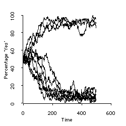
| Figure 1: Bimodal trends in opinion formation in a homogeneous population |
 |
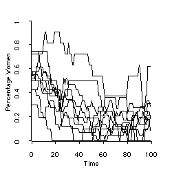
| Figure 2: Simulated distribution of percentages of women among teachers at 10 schools |
(mls-trace maths-mark)
The output will look like
Attribute MATHS-MARK of #<STUDENT-0> set to 57.829241873061605
Any number of attributes may be given in one call of mls-trace. To stop tracing an attribute, evaluate mls-untrace with the name of the attribute, or (mls-untrace) to stop all tracing.
(send a-teacher :from-lowers 'maths-mark)
would return a list of all the math marks of the students in a-teacher's class.
(send a-teacher :num-lowers)
returns the number of students in a-teacher's class.
(upper-attribute name-of-attribute)
(upper-attribute 'sex)
would return the sex of the student's teacher.
(prev-upper-attribute name-of-attribute &optional (time-steps 1))
(uniform lo-bound hi-bound)
(normal mean standard-deviation)
(chance odds)
(randomly-choose options...)
(randomly-choose lust gluttony envy pride)
will return one sin chosen randomly from the list.
(prob probability)
(prob 0.5) returns true half the time.
TIERNEY, L (1990) Lisp-Stat: an object-orientated environment for statistical computing and dynamic graphics, London: Wiley
TROITZSCH, Klaus G. (1996). Multilevel simulation, in K.G. Troitzsch, U. Mueller, G.N. Gilbert and J.E. Doran, Social Science Microsimulation Berlin: Springer
Return to Contents of this issue
© Copyright Journal of Artificial Societies and Social Simulation, 1998