©Copyright JASSS

JASSS logo ----

Marco A. Janssen (2009)

Understanding Artificial Anasazi

Journal of Artificial Societies and Social Simulation 12 (4) 13
<https://www.jasss.org/12/4/13.html>

For information about citing this article, click here

Received: 13-Jun-2009    Accepted: 27-Sep-2009    Published: 31-Oct-2009

PDF version


* Abstract

A replication and analysis of the Artificial Anasazi model is presented. It is shown that the success of replicating historical data is based on two parameters that adjust the carrying capacity of the Long House Valley. Compared to population estimates equal to the carrying capacity the specific agent behavior contributes only a modest improvement of the model to fit the archaeological records.

Keywords:
Replication, Model Analysis, Model-Based Archaeology, Population Dynamics, Social-Ecological Systems

* Introduction

1.1
The Artificial Anasazi model is one of the icon models of the agent-based modeling community. The model describes the population dynamics in the Long House Valley in Arizona between 800 and 1350 (Dean et al. 2000; Axtell et al. 2002; Gumerman et al. 2003). It is shown that by simple household rules on choosing locations for farms and settlements archaeological records on the occupation of the Anasazi in Long House Valley can be reproduced. The model analysis also shows that the abandonment of the valley around 1300 cannot be explained solely by environmental variations.

1.2
The model derived significant attention in the public media (Diamond 2002; Kohler et al. 2005) and is used of as one of the successful examples of agent-based modeling. The widely published figure of the fit of the simulation and the actual data suggest an astonishing performance of the model. In this paper an analysis is presented that aims to understand what makes the model so successful in fitting the actual data. We confirm the conclusions of the original paper, but show that the model itself has a modest contribution to this insight. The reason for this is that the model act as a smoothing function of the input data and has limited endogenous dynamics that contribute to the aggregated population data. Despite these drawbacks, the model might be a valuable starting point for more comprehensive models of societies in the prehistoric American South-West.

1.3
In recent years some important replications have been published in this journal. Edmonds and Hales (2003) had difficulty to reproduce the results from a paper published in Science (Riolo et al. 2001). Will and Hegselmann (2008) were not able to reproduce the results from Macy and Sato (2002) published in the Proceedings of the National Academy of Sciences. This paper focus on the results of Axtell et al. (2002) also published in the Proceedings of the National Academy of Sciences. This analysis shows once again that it is important to reanalyze each others' work in order to understand the findings of modeling studies.

1.4
The paper is organized in the following way. In the next section we present a detailed overview based on the Overview Design Details (ODD) protocol of Grimm et al. (2006). The original publications are used to provide this model description, and verified with the source code of the model. In the sections thereafter a model analysis using the Netlogo version of the model is presented. First we show that our Netlogo version produces the published results. Second, we redo the calibration procedure as presented in Axtell et al. (2002) and analyze which parameters contribute most to the performance of the model. Finally, we conclude the paper with a discussion of our findings.

* Model description

2.1
This section provides a model description of the main components of the model based on the ODD protocol of Grimm et al. (2006). This is a detailed presentation of the original model based on the documentation in Dean et al. (2000), Axtell et al. (2002), Gumerman et al. (2003) and verified with the source code of the model. The original model was implemented in Ascape. According to footnote m of Axtell et al. (2002) the source code of the model is available at http://www.brookings.edu/dynamics/models. When we started the replication of the Artificial Anasazi we found that the available version, implemented in Ascape, did not produce the results as published in Axtell et al. (2002). Having problems to replicate the published results, the authors were contacted and we communicated with the original programmer, Miles Parker, to solve the problems. The referred source code of the model is not available anymore via the link noted in Axtell et al. (2002). However, a new version of Ascape was launched as an open source project that contains the Long House Valley model ( http://sourceforge.net/projects/ascape/). We use this Ascape 5.0.1 implementation of the Long House Valley project to replicate the model in Net Logo 4.0.2. The replication kept as close as possible to the original code, but at times it was not clear which version of the original code was used to generate the original paper since alternate versions of the model are still extant in the code. This replication is based on eyeballing the results of the Ascape version versus the Netlogo version. Hence, the conclusions of the analysis discussed in this paper are based on the Netlogo version[1].

2.2
The model is implemented in NetLogo 4.0.2. The source code and a more detailed description of the model can be found in the model archive of openabm.org.

Agents and timescale

2.3
The model runs from 800 to 1350 in annual time steps. This is the time period in which the population in the Valley increased to about 250 households after which it declined. After 1300 there is no evidence of new constructions of houses in the valley. This suggests that there are no households living in the valley after 1300.

2.4
Each agent represents one household consisting of 5 persons. The composition of the households is not changing over time. Each household generates a demand for a certain level of food. To supply this demand the agent performs agriculture. The cell on which an agent farms is different than the cell an agent has its house. Each agent has its unique cell for farming, but more than one agent can have a house on a cell. There is no sharing of food between households, and storage of food is at the household level. Each household makes annual decisions on where to farm and where to settle. A household has an age, and a stock of food surplus from previous years.

Landscape

2.5
We present the landscape of the valley as used in the model. The landscape is defined on a map of 80 × 120 cells (Figure 1). Each cell represents a 100m × 100m space. Each cell is within one of the different zones of land: General Valley Floor, North Valley Floor, Midvalley Floor, Arable Uplands, Uplands Nonarable, Kinbiko Canyon or Dunes. These zones have agricultural productivity that is determined by the Palmer Drought Severity Index (PDSI) as discussed later.

2.6
The cells in the same zone differ a bit in the quality of the soil. At the start of the simulation the cells are initialized by adding a number drawn from the distribution n(0, σshv) where σshv is the spatial harvest variance. This generates a map of variability of soil quality within each zone of land.

Figure
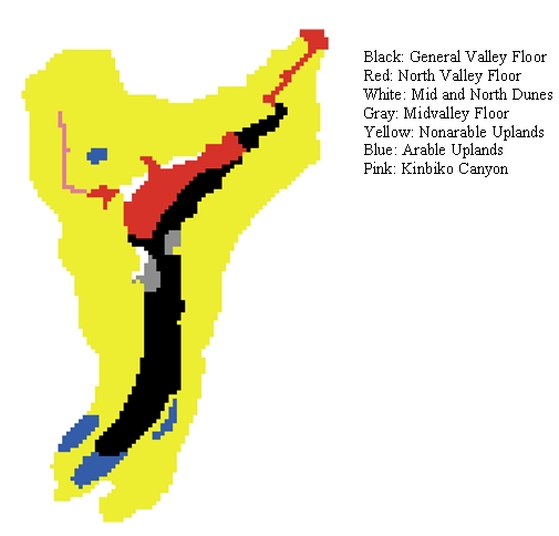
Figure 1. Different zones of land cover

Process overview and scheduling

2.7
Every year a sequence of actions are performed by the agents and the landscape. We discuss the relevant processes later in the paper, but to derive an overview of the sequence of actions, we first present the annual sequence of calculations:
  1. Calculate the harvest for each household
  2. IF an agent derives not sufficient food from harvest and storage OR the age is beyond maximum age of household THEN the agent is removed from the system
  3. Calculate the estimated harvest for next year based on corn in stock and actual harvest from current year
  4. Agents who expect not to derive the required amount of food next year will move to a new farm location and a plot to settle nearby.
  5. If a household is older than the minimum fertility age, there is a probability pf, that a new household is generated. The new household will derive an endowment of a fraction fcs of the corn stock.
  6. Update water sources based on input data
  7. Each agent, household, ages with one year.

2.8
The initial number of agents, households, is 14 in the year 800. These 14 agents are initialized by setting a household age from the uniform distribution [0, 29] and by setting the value of the corn stocks by the uniform distribution [2000, 2400].

Input

2.9
A number of files are imported with input data. Input data provides information which cells are water sources for which periods (rivers, wells, etc.). The main input is the so-called adjusted Palmer Drought Severity for each category of land cover. This annual index provides measurements of moisture conditions for agricultural activities. Thus for each cell information is available whether it was a wet/dry year for agricultural activities on that cell.

2.10
Furthermore, we have the following parameter values:

Table 2: Main parameters of the Artificial Anasazi model and their default values

VariableValue
Simulation period800 AD to 1350 AD
Nutritional need per household800 kg per year
Number of individuals per household5 persons
Maximum length of corn storage2 years
Harvest Adjustment Level1.00
Harvest Variance0.1
Start of Fertility Age16 years
End of Fertility Age30 years
Death Age (maximum age household)30 years
Fission Probability pf0.125
Corn stock given to new household fcs 0.33
Maximum distance between residence and farm1600m

Submodels

2.11
We will discuss some steps of the model in more detail. The base yield BY is defined by the yield y, quality of the soils in the cell q and the harvest adjustment level Ha,

BY = y × q × Ha

where yield y is defined for each zone and each PDSI index (Table 3). For each zone there is a table of yield levels for five levels of PDSI ( (-∞,-3], (-3, -1], (-1, 1), [1, 3), and [3, ∞)). Since the annual PDSI indicates whether the year was a wet year, high PDSI, or a dry year, low PDSI, the annual yield can change from year to year. The default value of Ha is 1 and is used for calibration.

Table 3: The yield levels for the different values of PDSI

Zones
PDSINorth and Mid Valley, Kinbiko CanyonGeneral ValleyArable UplandsDunes
(-∞,-3]617514411642
(-3,-1]719599479749
(-1,1)821684547855
[1,3)9888246591030
[3,∞)11539617691201

2.12
The harvest of a household H0 is equal to the base yield of the location BY adjusted by some annual variation of the harvest using a normal distribution and a standard deviation σahv

H0 = BY × (1 + n(0,σahv))

2.13
A household needs to derive 800 kg a year. Starting with the oldest stock of food, stored food is used to supply the demand. If the household can not meet the required nutrition needed after using storage and annual harvest, the household is removed from the system. In order to determine whether the agent should stay or go it estimates the harvest for next year on the same location. This estimation is the amount of stored corn left plus the expected harvest (equal to current harvest level).

2.14
An agent occupies a cell in the landscape for performing agriculture, and has a house on a different cell. A cell can be shared for housing, but agricultural plots are uniquely allocated to one agent. When an agent estimates that the amount of corn for the next time step is not sufficient to meet the demand, it will look for a new farm plot. Searching for a new farm plot is performed by identifying all unoccupied cells which produce more than the minimum nutrition requirement (800 kg) and which are within 1 mile from a water source. If there are multiple suitable locations, chose the one closest to the current location

2.15
Searching for a settlement is performed by executing the following conditions:
  1. The settlement location must be unfarmed (although it may be inhabited, i.e., multihousehold sites permitted).
  2. The settlement must be within 1 mile of the new agricultural plot selected.
  3. The settlement must be in a less productive zone than the new agricultural land selected.
If multiple sites satisfy these above criteria the location closest to the water resources is selected. If no site meets these criteria then first one looks at locations that meet condition i and ii. If still no site meets the criteria only sites who meet condition i are selected. Finally, if still no location is found, the agent leaves the system.

* Replicating the original results

3.1
In Axtell et al. (2002) a number of parameters were varied to calibrate the Artificial Anasazi model to the historical records. In fact these historical records are rough estimates of population numbers at selected years based on room counts and linearly extrapolated for the whole period. The default parameter values are Harvest Adjustment Level 1.0, Harvest Variance 0.1, Death Age (30 years), End of Fertility Age (30 years), and Fission Probability (0.125).

3.2
With these values they produce a population curve like Figure 2 (see also Dean et al. 2000).

Figure
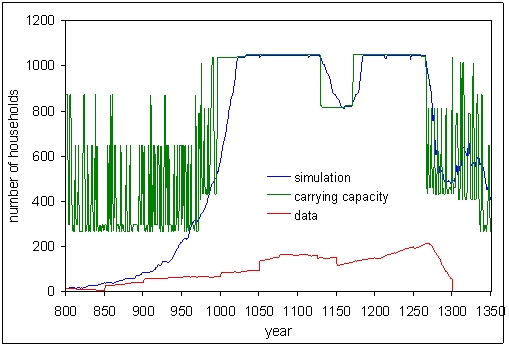
Figure 2. Results using the default parameter values. The blue line simulation is the number of households simulated by the model version as used in Dean et al. (2000). The red line data is the estimated number of households based on archaeological data. The green line carrying capacity is the amount of households possible on the landscape based on the number of cells that produces enough food for one household.

3.3
Carrying capacity in Figure 2 is defined as the number of cells which has a base yield equal or higher than the nutrition needs. These are potential farming plots. You see fluctuations in these values due to fluctuations in PDSI values in the data, and periods in which streams and alluviums exists. The simulated number of households grows towards the carrying capacity. When the carrying capacity drops, the population drops not immediately since stocks of corn buffer temporarily food shortages.

3.4
In Axtell et al. (2002) they calibrated the model by minimizing the difference of the simulated and historical data using 15 simulations. The Harvest Variance became 0.4 and the Harvest Adjustment Level was reduced to 0.6. The Fission Probability remained the same: 0.125. They assume variation in the agent population of the Death Age (30-36) and the End of Fertility Age (30-32). We use these parameter values and run our implementation 100 times (Figure 3). In Axtell et al. (2002) the best fit was published, but we see in Figure 3 that there is some variation in the results.

Figure
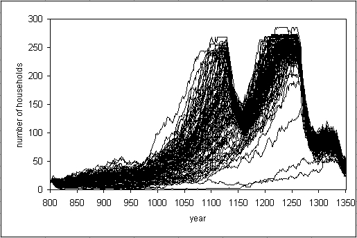
Figure 3. 100 runs with the "calibrated" Artificial Anasazi

3.5
In Figure 4 the best simulation of the 100 simulations is projected, with the historical data, and the carrying capacity. The best simulation is defined as the one with the smallest sum of squared differences between the simulated and historical data. The carrying capacity is changed due to changes in the Harvest Adjustment Level (if you assume people get only 60% of their harvest this reduces the carrying capacity) as well as the Harvest Variation. We see again that the simulated population grows towards the carrying capacity, and is somewhat delayed when the carrying capacity drops due to storage of corn.

Figure
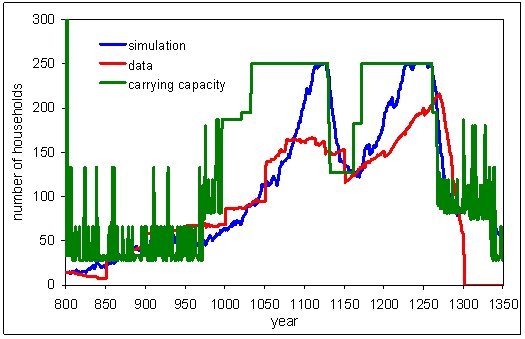
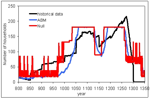
Figure 4. Simulated ("best" fit) and historical data and the carrying capacity for the parameter values from Axtell et al. (2002)

* The Original Model Calibration Revised

4.1
What leads to the good fit of the simulation with the aggregated population data? We repeated the model calibration for an extensive parameter space. We do not assume heterogeneity for Death Age, End of Fertility Age and Fission Probability like Axtell et al. (2002) in order to reduce the number of parameters. We tested the effect on the two parameter settings used in the previous section and did not found a significant difference in the results with and without heterogeneity of these three parameters. The model is run 15 times for each variation of the parameter values like Axtell et al. (2002). Besides calculating the fit between the simulated and actual population numbers, we also calculated the fit between the simulated carrying capacity and the actual population numbers. The simulated carrying capacity does not depend on agent-behavior, only on the values of base yields (BY).

4.2
For exploring the parameter space of the model, we assume that the Death Age and End of Fertility Age can be 26, 28, 30, 32, 34, 36, 38 and 40. We assume that the End of Fertility Age can never be larger than Death Age which leads to 36 combinations. We will vary the Fission Probability between 0.095 and 0.185 with steps of 0.015.

4.3
In the default simulation with Harvest Variance 0.1 and Harvest Adjustment Level 1, the potential number of households is around 1050 in 1260 while the data indicates numbers just above 200. The reason for these numbers is that 406 cells in the North and Mid Valley and the Kinbiko Canyon receive 1153 kg, 637 cells in the General Valley receive 961 kg and 50 cells in the Dunes of the North and Mid Valley receive 855 kg per cell.

4.4
The minimum level of production of a cell to be self sufficient is 800 kg. For the most productive regions, the North and Mid Valley and the Kinbiko Canyon, to produce less than 800 kg, 30% of the potential harvest (1153 kg), needs to be lost. Thus if we reduce the Harvest Adjustment Level to 800/1153 = 0.7 with a small variance, we still get 406 potential cells available for agriculture. If we add a Harvest Variance to the cells, not all 406 potential cells will generate more than 800 kg. On the other hand, cells in less productive regions, like the General Valley, will have individual cells above 800 kg. We decided to explore the range of Harvest Adjustment Level between 0.54 and 0.7 (in steps of 0.02) and a Harvest Variance between 0 and 0.7 (in steps of 0.1), which produces carrying capacities around 200 agents in 1260.

4.5
The carrying capacity model is only dependent on the parameters Harvest Variance and the Harvest Adjustment Level. In fact, we can call this model a null model, since it is a simpler representation of the system, no agent-behavior, to retrodict the aggregated population numbers.

4.6
This leads to 18144 parameter combination and for each simulation the following metrics are calculated:

4.7
This analysis was done with a replication of the Artificial Anasazi model. In Table 4 the best fit for the replicated model, the carrying capacity model and the results presented in Axtell et al. (2002). It is interesting to see that the replicated model and the carrying capacity model have the same optimized parameter setting which suggest that fitting the carrying capacity to the population estimates is key to get a good fit between the replicated model and the data. There are a few differences in the parameter estimates between the replicated model and the original model. One reason might be the use of heterogeneity in the original model. Another reason might be that our replication is not exact. We know the exact outcome of the calibration process as performed by Axtell et al. (2002). However, we do not know which parameter values have been explored in their calibration process.

Table 4: Optimized parameter settings based on the average over 15 runs of the model for the replicated model, the carrying capacity model and the original model. The values between brackets in the last 2 columns refer to the lower and upper range of the uniform distribution of the parameter values.

L1 and L2 population and L2 carrying capacityL1 carrying capacityL1 population
(Axtell et al. 2002)
L2 population
(Axtell et al. 2002)
Death age38(30-36)(25-38)
End of Fertility Age34(30-32)(30-38)
Fission Probability0.1550.1250.125
Harvest Adjustment0.560.540.60.6
Harvest Variance0.40.40.40.4

4.8
In Figures 5-9 we depict the relative fit of the replicated model and the carrying capacity model as a function of the different parameters. For each parameter we look for each specific value what has been the best average fit. Then we divide L1 and L2 values by the best fit derived (replicated and carrying capacity models). Hence the best fit will have a value 1. A value 2 means that the best fit found for parameter value (say Harvest Variance = 0.5) is twice the size as the best fit for all parameter values of Harvest Variance. Each figure shows the relative improvements of the best fit for changing the parameter values. Some parameter values result in large changes in the best fit, while others are relative insensitive.

4.9
Death Age lead to the best fits with values of higher than 34 while for End of Fertility Age a value of higher than 30 leads to the best values. Beyond these values they reach a plateau where no improvement is found. Values beyond 40 are not explored because of the infeasibility of such assumptions of this population. Fission Probability enters a plateau for values of 0.125 and higher.

4.10
The relative metrics of the carrying capacity models are 10% (L1) to 50% (L2) higher than the replicated model. Nevertheless, we see clearly from Figures 5-7 for which values the replicated model outperforms the carrying capacity model (Death Age 36+; End of Fertility Age 30+; Fission Probability 0.125+).

4.11
The story for Harvest Adjustment Level and the Harvest Variance is different. Those values affect the carrying capacity. We see a steep improvement of the relative fit if the Harvest Adjustment Level declines from 0.7 to 0.54. The best fit is derives for values 0.54 and 0.56. The same is true for Harvest Variance. For value 0.4 the relative fit is close to optimal, but for higher and lower values the relative fit dramatically worsen. Figures 8 and 9 show that the improvement of the fit is caused largely by a better carrying capacity model. Note that the original model in Dean et al. (2000) used Harvest Adjustment Level equal to 1 and Harvest Variance equal to 0.1.

Figure
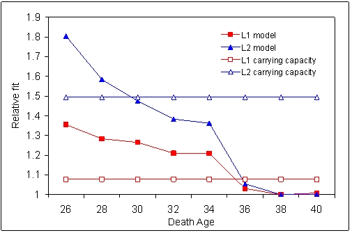
Figure 5. Relative fit of the replicated Artificial Anasazi model as a function of the parameter Death Age. The values are the best average over 15 runs for all simulations with that particular value of Death Age.

Figure
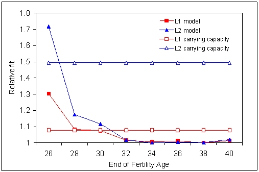
Figure 6. Relative fit of the replicated Artificial Anasazi model as a function of the parameter End of Fertility Age. The values are the best average over 15 runs for all simulations with that particular value of End of Fertility Age.

Figure
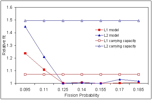
Figure 7. Relative fit of the replicated Artificial Anasazi model as a function of the parameter Fission Probability. The values are the best average over 15 runs for all simulations with that particular value of Fission Probability.

Figure
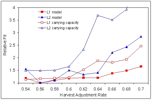
Figure 8. Relative fit of the replicated Artificial Anasazi model as a function of the parameter Harvest Adjustment Level. The values are the best average over 15 runs for all simulations with that particular value of Harvest Adjustment Level.

Figure
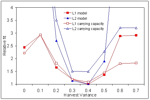
Figure 9. Relative fit of the replicated Artificial Anasazi model as a function of the parameter Harvest Variance. The values are the best average over 15 runs for all simulations with that particular value of Harvest Variance.

4.12
Like Axtell et al. (2002) we depict the best individual run and show also the results for the carrying capacity (Figure 10). Both fits look similar, although the carrying capacity model is more erratic since it looks at the number of suitable patches in a year for agriculture, and the agent-based model smoothens out the population by having storage and natural reproduction.

4.13
The systematic calibration leads to some artifacts. Since the population is following the carrying capacity, adjusting Harvest Variance and Harvest Adjustment Level to a carrying capacity scenario leads to a trajectory that meets the average of the two peaks. Since the carrying capacity of the two peaks are the same, we will always get a too high population level generated for the first peak (1030-1130) and a population level for the second peak that stays below the maximum of the second peak (1180-1260). In all simulations the population and carrying capacity remain positive after the archaeological data suggest the abandonment of the valley.

Figure
Figure 10. Best individual run for the agent-based model and the population numbers according to the carrying capacity model using the L2 metric and the parameter values from the second column.

* Discussion

5.1
The main message of Axtell et al. (2002) is that environmental factors only cannot explain the sudden abandonment of the Long House Valley around 1300. Our analysis confirms this result. Figure 2 of Axtell et al. (2002) presents a close fit between the archaeological record and the simulation model and this might provide the suggestion that the model is very accurate in describing the population dynamics of the Long House Valley. Our analysis shows that this success is driven by adjusting the carrying capacity of the simulated valley. The adjustment of the variables that determine the demographics of the agents are less important. As long as we assume that households have a maximum existence of more than 30 years, and another household is reproduced on average each 6 to 8 years, the model will generate population numbers that follow the carrying capacity. As long as the carrying capacity approximates the population levels, the model produces a close fit with the data. The agent-based model acted as a smoothing function for the irregular carrying capacity levels. The population could not increase faster than the natural reproduction rate, and the decline of the population is buffered by storage of corn.

5.2
It should be noted that although our model analysis confirms the finding of Axtell et al. (2002), this does not mean that the discussion on the relevance of droughts and other environmental influence on the abandonment of settlements in the Long House Valley is settled. See for example Kohler et al. (2008) for a recent discussion on new insights on the importance of long lasting droughts in the North American South West.

5.3
As Axtell et al. (2002) acknowledges there are many more additions to the model possible such as social interactions between households (reciprocal exchange of food, kinship relations). It is also likely that households do not make decisions to leave the valley completely independent of other households if they are part of a social fabric. More complex arrangements, especially exchange in social networks, have been included in more recent models on the ancient US south west (Reynolds et al. 2003) and Janssen (in review).

5.4
This leads to a broader topic for agent-based modeling, and model based archaeology in particular (Kohler and van der Leeuw 2007). Within model-based archaeology two approaches can be identified: (1) detailed data-driven simulation models that mimic observed trends like population numbers, (2) stylized models that are informed by empirical data but explore a broader domain of possible social-ecological systems. Which approach is the most appropriate depends on the research question at hand. The fact that the Long House Valley abandonment can not be explained by environmental factors is demonstrated by the original Artificial Anasazi, but it could also be explained by calculating the carrying capacity of the valley. A more comprehensive question like whether exchange networks increase the resilience of settlements in the US south west may need to be addressed by a series of models, including stylized models that simulate various possible landscapes. Such a model would be based on assumptions that rely less on quantitative measurements like the Artificial Anasazi, but more on ethnographic interpretations of possible social mechanisms that can not be verified (no written records on social practices of the societies which were collapsed before European contacts).

5.5
Retrodicting aggregate population dynamics of the Long House Valley has been very successful. However, these results are mainly the consequence of tweaking the carrying capacity to appropriate levels. The use of modeling in understanding ancient societies is still in its infancy. Instead of fitting models to the material culture I would propose to focus on stylized theory based models which are grounded in the knowledge we have derived from material artifacts and ethnographic records. Such stylized models may produce system dynamics for different types of societies in different types of landscapes, and can be tested on various societies for which comprehensive data is available, like the Long House Valley. With such an approach we may derive knowledge of social-ecological systems that is applicable beyond a specific archaeological site.

* Acknowledgements

The author would like to thank the National Science Foundation and its Human Social Dynamics Program (NSF-BCS 0623162). Furthermore, Sean Bergin helped with the digital excavation and interpretation of the Ascape version of Artificial Anasazi which made it possible to reimplement the model in Netlogo. Original Artificial Anasazi programmer Miles Parker provided helpful feedback to the replication attempts and by cleaning up the code for the launch of the new Ascape edition. The author also thank the three anonymous reviewers for their detailed and helpful reviews.


* Notes

1The description of the model in Axtell et al. (2002) is somewhat confusing. On a few places it is suggested that household composition is explicitly taken into account, while the code only considers households of five unspecified household members:
"Each household that is both matrilineal and matrilocal consists of 5 individuals. Only female marriage and residence location are tracked, although males are included in maize-consumption calculations. (Table 1, page 7276)"
"A household fissions when a daughter reaches the age of 15. (Table 2, page 7277)"
The code uses an annual time step while the paper suggests that there are monthly time steps:
"A second clock runs from April to April and reduces the amount of maize in storage by 13.33 kg of maize per month per individual in the household. (Table 3, page 7277)"
We follow the code instead of the description in performing our analysis.


* References

AXTELL R L, Epstein J M, Dean J S, Gumerman G J, Swedlund A C, Harburger J, Chakravarty S, Hammond R, Parker J, and Parker M. (2002) Population Growth and Collapse in a Multi-Agent Model of the Kayenta Anasazi in Long House Valley. Proceedings of the National Academy of Sciences 99(3): 7275-7279.

DEAN J S, Gumerman G J, Epstein J M, Axtell R L, Swedlund A C, Parker M T, and McCarroll S. (2000) Understanding Anasazi Culture Change Through Agent Based Modeling in Dynamics in Human and Primate Societies: Agent Based Modeling of Social and Spatial Processes, T. Kohler and G. Gumerman (eds.), Santa Fe Institute. New York & London: Oxford University Press.

DIAMOND, J. (2002) Archaeology: Life with the artificial Anasazi, Nature 419: 567-569.

EDMONDS, B and HALES, D (2003) Replication, Replication and Replication: Some Hard Lessons from Model Alignment, Journal of Artificial Societies and Social Simulation 6 (4) 11 https://www.jasss.org/6/4/11.html.

GRIMM V, Berger U, Bastiansen F, Eliassen S, Ginot V, Giske J, Goss-Custard J, Grand T, Heinz S, Huse G, Huth A, Jepsen J U, Jørgensen C, Mooij W M, Müller B, Pe'er G, Piou C, Railsback S F, Robbins A M, Robbins M M, Rossmanith E, Rüger N, Strand E, Souissi S, Stillman R A, Vabø R, Visser U, DeAngelis D L. (2006) A standard protocol for describing individual-based and agent-based models. Ecological Modelling 198:115-126.

GUMERMAN G J, Swedlund A C, Dean J S, and Epstein J M (2003) The Evolution of Social Behavior in the Prehistoric American Southwest. Artificial Life 9: 435-444

JANSSEN, M A Population aggregation in the ancient arid environments, in review

KOHLER, T A , Gumerman, G J and Reynolds, R G (2005) Simulating ancient societies, Scientific American 293(1): 76-82

KOHLER, T A and van der Leeuw, S A (eds) (2007) The Model-based Archaeology of Socionatural Systems, School for Advanced Research Press.

KOHLER, T A, Varien M D, Wright A and Kuckelman K A (2008) Mesa Verde Migrations: New archaeological research and computer simulation suggest why ancestral Puebloans deserted the northern Southwest United States. American Scientist 96:146-153

MACY M and Sato Y (2002) Trust, cooperation and market formation in the US and Japan. Proceedings of the National Academy of Sciences, 99, pp. 7214-7220.

REYNOLDS, R G, Kohler, T A and Kobti, A (2003) The Effects of Generalized Reciprocal Exchange on the Resilience of Social Networks: An Example from the Prehispanic Mesa Verde Region, Computational & Mathematical Organization Theory, 9, 227-254

RIOLO, R L, Cohen, M D and Axelrod, R (2001), Evolution of cooperation without reciprocity. Nature, 411:441-443.

WILL, O, and Hegselmann, R (2008). 'A Replication That Failed - on the Computational Model in 'Michael W. Macy and Yoshimichi Sato: Trust, Cooperation and Market Formation in the U.S. and Japan. Proceedings of the National Academy of Sciences, May 2002''. Journal of Artificial Societies and Social Simulation 11 (3) 3 https://www.jasss.org/11/3/3.html

----

ButtonReturn to Contents of this issue