©Copyright JASSS

JASSS logo ----

Paivi Mattila-Wiro (2009)

Income Distribution Effects of a Finnish Work Incentive Trap Reform

Journal of Artificial Societies and Social Simulation 12 (3) 3
<https://www.jasss.org/12/3/3.html>

For information about citing this article, click here

Received: 02-Sep-2008    Accepted: 04-May-2009    Published: 30-Jun-2009

PDF version


* Abstract

The present study concentrates on the income distribution effects of A Finnish Work Incentive Trap Reform started in 1996. I estimate how the reforms made have affected income levels and income inequality - the distribution of economic wellbeing. I look at the effects both without and with behavioral response. The data used is the Income Distribution Statistics of Statistics Finland from the years 1996 and 1998. The empirical part of the study is based on a microsimulation model. The method of microsimulation is a powerful tool for the analysis of ex post evaluation of policy reforms. However, the method is rarely and on very few occasions applied in Finland. The results drawn without behavioral response show that the 1996 data with the 1998 legislation produces lower values for income inequality measures and higher average income levels for almost all income decile groups compared to those with the 1996 legislation. However, the changes are very small. When the labor supply effect is included, the lowest incomes rise only very little (in fact, hardly at all) and the Gini coefficient remains unaltered.

Keywords:
Work Incentive Trap Reforms, Microsimulation, Disposable Income, Economic Well-Being, Inequality, Poverty

* Introduction

1.1
Progressive taxation, together with the income deductibility of social benefits, can create a situation, an incentive trap, where working does not provide a higher level of income compared to income offered by social security. In Finland the economic depression in the 1990s with serious unemployment, the financial problems of the public sector and the complications of the labor market raised an effort to remove work incentive traps[1]. The number of people employed needed to be increased and the number of people living on social security needed to be cut. By cutting the incentive traps it was anticipated that the price of labor and social security expenses would drop, domestic demand, demand for labor and productivity, would rise and this would eventually lead to the improved livelihood of all population groups. Work incentive trap reforms are particularly intended to enhance the labor supply of those unemployed or otherwise out of the labor force.

1.2
Lipponen's first government appointed in 1995 the so-called Incentive Trap Task Force (here Task Force) to discuss how the compatibility of taxes, social security transfers and public service payments could be improved to decrease incentive traps and increase the profitability of working. Income provided by work should always exceed income provided by social benefits, and working extra hours or otherwise receiving extra income should increase the current disposable income. Basically, the Task Force was trying to consolidate the aims of efficiency and equity, efficiency in the sense that people would prefer working to living on social security and equity in the sense that one of the principal objectives of the social security system is equal distribution of income (Prime Minister's Office 1996; Laine and Uusitalo 2001) .

1.3
Efficiency of the reforms has already been explored in detail, as an example, in the studies of Laine and Uusitalo ( 2001), Kurjenoja (2000) and Kurjenoja (2004). But the equity of the reforms has gained much less attention, regardless of the fact that it is of crucial importance to analyze the distributional effects of tax and social security reforms in order to target and implement successful reforms in the future.

1.4
The present study concentrates on the equity of the work incentive reforms by looking at how the reforms have affected income levels and income inequality - the distribution of economic wellbeing. I first look at the changes without behavioral response and, secondly, the changes with labor supply effect (behavioral response). The study includes the main work incentive trap reforms and those tax reforms that were implemented at the same time with the work incentive trap reforms. Other changes in the social security system or in taxation are excluded.

1.5
The data used is the Income Distribution Statistics of Statistics Finland from the years 1996 and 1998. Important contribution of the paper is a methodological one. The empirical part of the study is based on a microsimulation model developed by and explained in Laine and Uusitalo (2001). This microsimulation model, originally intended to study labor supply and marginal tax rates, has been converted and partly rewritten to produce variables needed in the analysis of income distribution. By using the simulation model it is possible to separate the effects of the incentive trap reforms on income distribution from the effects brought about by other changes in the economy and society.

1.6
The study starts with a short background review of work incentive traps in general. A description of the Finnish Work Incentive Trap Reform follows as well as a summary of the effects of these reforms. Thirdly, the empirical research strategy is described in detail. Next, the effects of the reforms on income levels and income inequality is reported, without and with the behavioral responses. Finally the main results and conclusions are drawn.

* The Finnish Work Incentive Trap Reform

2.1
Work incentive traps are normally divided into two. Unemployment trap means that reservation wages are higher than wages offered to the unemployed and thus working does not pay off. Income trap means that incentives to carry out extra work are very small because extra taxable income results in higher taxes, lower social benefits and/or higher public service payments. In an extreme case, extra income may lead to diminishing disposable income.

2.2
Reservation wages can be cut through a reduction in the level of social security (as an example by lowering the degree of compensation) or by tightening the eligibility requirements (limiting the number of recipients and excluding them from the scope of the benefit) and possibly simultaneously cutting taxation. The alleviation of the income trap problem means reducing high marginal taxation rates, which requires the lowering of the means test of social transfers, dropping the income contingent of service charges and cutting the progressivity of taxation (Niinivaara 1999; Laine and Uusitalo 2001; Prime Minister's Office 1996; Heikkilä 1997) .

2.3
When comparing the aims of cutting incentive traps and having equal income distribution in society, it is well known that efforts required by one of the aims easily worsens the possibilities in achieving the other. As an example, increasing work incentives presumes a decrease in taxes and, as a consequence, income inequality increases. On the other hand, reduction in income inequality by increasing the progressivity of taxation may lead to severe incentive traps (see for exampleUusitalo 1997).

2.4
In tackling the work incentive problem in Finland, the Task Force selected two principal goals. Firstly, the consistency of minimum security had to be increased and, secondly, work incentive traps of low- and middle-income earners needed to be cut. It is primarily low- and middle-income earners whose income is supplemented with income transfers aiming at equalizing income distribution. The target group was especially the working age population. The Task Force suggested main modifications to the housing allowance, unemployment assistance, payments of the municipal day-care, home care subsidy and the earned income deduction of municipal tax. Pensions were not included in the agenda and neither were incentive traps created by earnings-related unemployment benefit. The latter problem was already processed by another working group (Prime Minister's Office 1996; Laine and Uusitalo 2001; Heikkilä 1997) .

2.5
The basic guideline of the Task Force was that working is a primary source of economic wellbeing and this status should be maintained in relation to social security. Participating in paid work was seen as the best way of preventing marginalization in society. Thus, the focus was essentially on reducing unemployment traps since their effect on people's wellbeing was considered to be greater than the effect of income traps. The reforms were accepted by Parliament in 1995 and the implementation started between 1996 and 1998. However, not all of the suggested reforms were implemented (Prime Minister's Office 1996; Laine and Uusitalo 2001; Heikkilä 1997).

2.6
Earlier studies on incentive traps have explored the whole range of tax and benefit reforms carried out in Finland and the consequences of these reforms. As an example, many studies have been written about the cuts in social security made in the 1990s, the background of and justification for these cuts, the economic environment before and during the cuts and the effect of the cuts on the well-being of households (see for exampleKosunen 1997; Heikkilä and Uusitalo 1997). The income distribution effects of cuts have been examined (seeUusitalo 1997) but only until the year 1995. Kurjenoja (2000) has studied the work incentive trap reforms made between 1996 and 1998 and their effect on the disposable income of two-parent two-child households living in Helsinki and in single parent families with one or two children. Laine and Uusitalo (2001) concentrated in changes in reservation wages and labor supply as a result of work incentive reforms. There are no earlier studies on changes in the distribution of economic wellbeing as a result of the Finnish Work Incentive Trap Reform.

2.7
As an example of research on incentive traps carried out in other countries, Duncan and MacCrae (1999) have studied the household labor supply effects of Working Family Tax Credit in the UK. They focused especially on lone parent households. Blundell, Duncan and Meghir (1998) have explored the labor supply responses of the UK tax reforms of married or cohabiting women. In Norway Aarbu and Thoresen (1997) have studied the effect of the Norwegian Tax Reform on income changes and income distribution.

Summary of the effects of the reforms

2.8
A detailed description of the each reform made can be found in the Appendix 1. As a summary, it can be claimed that the reforms implemented led to decreased taxes, increased earned income deduction and lowered income contingent on unemployment assistance and day-care payments. Niinivaara (1999) explains that in reducing unemployment traps the objectives drawn were achieved. The possibilities for an unemployed person to improve their livelihood by extra income are now better than they were before the reforms. Furthermore, the reservation wages dropped significantly in all families, whether it was a single parent, two parent family, family with more than one child or a single adult household (Niinivaara 1999).

2.9
Results in reducing income traps were more moderate. Cutting the high marginal tax rates did not succeed as well as expected. The marginal tax rates are lowered around 2-3%. This does not have a real effect on decreasing income traps (Niinivaara 1999). According to Kurjenoja (2000), incentive traps have remained for young families, single parents with day-care age children, and for families where one spouse receives labor market support and the other one is a wage earner. The reforms did not concentrate only on low income households, since families with two adults and children are not all at the low end of the income distribution.

2.10
Laine and Uusitalo (2001) summarize that the reforms positively affected work incentives and the labor supply. I now turn to analyze the effect of the reforms on income levels and on income inequality. The research strategy is first explained in detail in the following section.

* The empirical research strategy

3.1
The present paper focuses on changes in the distribution of economic wellbeing created by A Finnish Work Incentive Trap Reform. I especially analyze the changes in income inequality and in income levels. The years included are 1996 and 1998. Year 1996 represents the period before the reforms and 1998 the year when the reforms had already been implemented. The analysis is carried out in steps, emphasizing two perspectives, changes without behavioral adjustment and changes with behavioral responses.

3.2
The data used is the Income Distribution Statistics (IDS) of Statistics Finland. IDS includes the level, formation and distribution of income among households and the economically active population. It is based on interviews and administrative records. The sample size is about 10 000 households each year, which makes around 25 000 individuals. Half of the sample alters each year and the same households appear in two succeeding years. The data includes sample weights which help in calculating results at the level of the population. The data covers all income items affecting disposable income and received income transfers. The data has around 700 variables (Statistics Finland 2003).

3.3
In the present paper, household disposable income is made comparable by using the equivalence scale

Equation (1)

where W is the total income of a household and S is the number of household members. When transferring monetary figures between years, the money values have been made comparable by using the cost of living index. Ultimately, all figures correspond to year 2000 Euros. Figures are weighted. It is always mentioned whether the figures are calculated directly from the Income Distribution Statistics or whether the microsimulation model is used. The income levels are described by decile group means (and medians in some cases). The income inequality measures chosen are the GE(2)-ratio[2] and the Gini coefficient[3]. The Gini coefficient is not sensitive to observations on the edge but it shows the general trend of inequality, which is important when looking at the changes over the years. Other factors than work incentive reforms and changes in taxation, influencing the income and income distribution, are not analyzed here. In calculating the taxes the simulation model does not include taxes on capital or wealth tax. Thus, from the tax parameter in the original data the same items are eliminated. Reforms concerning capital taxation are not included.

3.4
The microsimulation model by Laine and Uusitalo (2001) is used in the paper's calculations. The model is basically a tax-benefit calculation program (the examples and the calculations of the microsimulation model are based on the payments applied in Helsinki). However, in the present paper the model is applied to examine the distributional effects of A Finnish Work Incentive Trap Reform. This means that the microsimulation model has been modified for the purpose of the study. The model has been put together from separate parts of the original model and every step of the model is checked. The microsimulation model is revised and partly rewritten to calculate the variables needed, for example, household disposable income. The microsimulation model combines micro-data (here Income Distribution Statistics) with tax and benefit rules describing each year's existing policy. This means that it is possible to combine the 1996 data with the 1998 legislation and vice versa.

3.5
The analysis starts by comparing household level disposable income figures and income inequality indicators calculated from the Income Distribution Statistics directly and the corresponding figures obtained by using the microsimulation model. This analysis includes the whole population. Only those households having a disposable income level equal to zero have been deleted (the number of these households vary between years and between cases studied and is not considered to be significant in any of the calculations). Household disposable income is a measure of the monetary resources available to a household at a predetermined time. Disposable income is a central term when analyzing work incentive traps since disposable income reflects a household's economic situation after all income, transfers, taxes and payments (Kurjenoja 2000). The disposable income of a household is formed by totalling household aggregate earned income, capital income and transfers received deducted by paid taxes.

3.6
Secondly, I look at what effects the changes in the system of social benefits and taxation has brought about in income levels and in income inequality. I analyze the effects of all the reforms on the whole population without behavioral response. I calculate household disposable income figures by combining year 1996 data with year 1998 legislation and year 1998 data with year 1996 legislation. Legislation means here the rules and regulations for taxation and social security payments. When taking the pre-reform population (1996) and post-reform legislation (1998) the 'pure' effect of changed legislation on incomes and income inequality can be seen. On the other hand, when taking pre-reform legislation (1996) and post-reform population (1998) the effect of demographic changes on income distribution is obtained. All the incomes in the tables are yearly figures.

3.7
Thirdly, I look at the behavioral response the reforms have generated and estimate a labor supply model. The obtained labor supply estimates are used to calculate the fitted value of months worked for the years 1996 and 1998 and for each individual. The fitted values of months worked are again applied to assess the effects of the reforms on each individual's yearly income. Finally, individual level information is aggregated at the household level and by using the household disposable income variable it is possible to calculate how the labor supply changes have affected income inequality measures and decile group means. The process of forming the labor supply function and calculating the behavioral responds are explained in detail in the following chaptes.

* Effects on income levels and income inequality

Changes without behavioral response

4.1
When we compare the mean and median values of household disposable income figures computed first from the Income Distribution Statistics (IDS) directly and secondly from the microsimulation model we can see from Table 1 that the microsimulation model systematically overestimates the mean and median values of disposable income (compare results between IDS: 1996 data and simulation: 1996 data/1996 legislation). The overestimation is especially significant in the case of low income decile groups. The tendency to overestimate the lowest incomes is quite typical in the case of microsimulation models. However, if these errors were eliminated, it would increase the usefulness of the simulation model[4].

Table 1: Mean and median household disposable income (and standard errors of the mean) by income decile groups in 1996 and 1998 (in year 2000 euros)


IDS* 1996 data


Simulation**
1996 data,
1996 legislation
IDS*
1998 data
Simulation**
1998 data,
1998 legislation
Simulation**
1996 data,
1998 legislation
Simulation**
1998 data,
1996 legislation
DecileMeanSEMedMeanMedMeanSEMedMeanMedMeanMedMeanMed
175896481379043967676826982399630100349103968891699679
21066819106841204912093108752110881124891251312072121191225912269
31237016124441358213602127121812708140021401513649136791383913854
41389615139271486914851143861714376154441548014944149311534915383
51527214152451620116211160681616083169311694816282162781683716840
61676714167871757317567177891817786185011849717663176631840418409
71835617183451908619051196962019672202692024319195191552013820120
82045523203922113821119220892522044225692253221256212592245122410
92359933235472405123900255753825496259802590424156240182586725797
10346823373063935219314964102082133740427283463335287314454259834510

Source: Author's calculations from the Income Distribution Statistics Note: *Income Distribution Statistics **Microsimulation model results

4.2
Several reasons can be found to explain the over-estimation problem of the microsimulation models. Some of the elements of social security can have variation between cities. The microsimulation model used here is based on the social security payments applied in Helsinki and these payments are not necessarily the same across the country. Secondly, social assistance as means-tested benefit is very problematic to calculate. Many of those eligible for social assistance have not either applied for it or received it. In the microsimulation model, social assistance is targeted to everyone eligible. This assumption has to be made since there is no information on those who are eligible on a certain social assistance but who do not apply for it for one reason or another. In this sense the simulation model assumes that people know what social assistance they are eligible for and also receive all of them. This means that the simulation model provides a framework with which to study the behavioral participation decision[5]. Finally, in the microsimulation model, the housing allowance is targeted to everyone eligible for this allowance according to their income. Similarly with social assistance, in reality, not all individuals eligible for housing allowance have applied for it or received it. However, it is evident that the method of microsimulation is a powerful and valuable tool for the analysis of ex post evaluation of policy reforms.

Table 2: GE(2) and Gini coefficient for 1996 and 1998, IDS results and microsimulation model results


Year of the data

IDS results*
Simulated results**,
Year of the legislation
19961998
GE(2) x 100Gini x 100GE(2) x 100Gini x 100GE(2) x 100Gini x 100
199611.1322.499.5420.339.520.31
199823.9524.9825.6823.5625.1623.17

Source: Author's calculations from the Income Distribution Statistics
Note:
*Calculated from the IDS data directly,
**Calculated by using the microsimulation model

4.3
Table 2 shows GE(2) and Gini coefficient values for 1996 and 1998 at the household level. First, the results are drawn from the IDS data directly, and GE(2) results in a value of 11.13 and the Gini coefficient in a value of 22.49 in 1996. For 1998 the corresponding figures are 23.95 and 24.98. Secondly, the same indices are calculated by using the microsimulation model and the result changes to GE(2) 9.54 and the Gini coefficient 20.33 in 1996 and GE(2) 25.16 and the Gini coefficient 23.17 in 1998. In both cases the income inequality measures are higher in 1998 than in 1996. This trend is verified by many other studies as well. As expected, in 1996, the income inequality measures calculated from the original data are higher than those drawn as a result of a simulation. In the case of 1998 the simulation process has resulted in a higher value for the GE(2) ratio but a lower Gini coefficient value compared to those calculated from the IDS data directly.

4.4
The Table 1 reports at the household level and at the whole population level, the mean and median incomes of income decile groups for the 1996 population by applying the year 1998 legislation. The post-reform legislation is applied to the pre-reform population. The same procedure is carried out for 1998 data using the 1996 legislation. The figures are calculated from the Income Distribution Statistics (IDS) directly and from the microsimulation model.

4.5
The results show that mean and median income values of the decile groups for 1996 data with the 1998 legislation are almost systematically higher than the corresponding figures when combining the 1996 data with the 1996 legislation. The only exception is the median income of the tenth decile group. This indicates that the 1998 legislation produces higher average (mean and median) income levels for almost all income decile groups compared to those with the 1996 legislation. However, the mean income of middle and high decile groups, especially decile groups from 5 to 9, increases more than the mean income of income decile groups from 1 to 4. This result suggests that the middle and high income earners have benefited more from the reforms than have the low income earners. Furthermore, the increase in the mean and median income of the lowest income decile groups is so small that it cannot be taken as reliable evidence of the success of the reforms (meaning that reforms had been beneficial especially for low income earners).

4.6
Both of the income inequality measures (Table 2) are somewhat lower in case of the 1996 data with the 1998 legislation (9.50 and 20.31) than in the case of the 1996 data with the 1996 legislation (9.54 and 20.33). However, the figures differ only slightly from each other and therefore the result does not convince us that the reforms have been successful in equalizing income distribution.

4.7
When taking the 1998 data and combine that with the 1996 legislation (Table 1) the effect of demographic changes again results in higher mean and median decile group values compared to corresponding results when taking the 1996 data with the 1996 legislation but lower values compared to those produced by combining the 1996 data with the 1998 legislation. On the other hand, both the income inequality indicators address the increase in income inequality as a result of demographic changes (25.68 and 23.56) compared to the 1996 data with the 1996 legislation (9.54 and 20.33).

4.8
Therefore, it can be claimed that even when the 1998 legislation seems to produce lower income inequality indicators than the 1996 legislation, the demographic effect of the year 1998 operates in the other direction and raises the income inequality measures.

Labor supply

Formation of the labor supply variables

4.9
The analysis of the behavioral response starts with the estimation of a labor supply model. Change in the labor supply is regarded as the most important behavioral effect of the work incentive reforms. The time period from 1996 to 1998 is considered to be long enough to study the behavioral changes since there has been some time for individuals to adjust their behavior to implemented reforms. The estimation of the labor supply is carried out by following, as closely as possible, the steps and method explained in Laine and Uusitalo (2001) in order to maintain the usability of the tax-benefit microsimulation model.

4.10
I estimate here the effects of the changes in the tax- and social security system on the number of working months, the dependent variable. Working months is a natural choice in regard to many social security regulations, since sometimes only the fact whether an individual is employed or not matters, not the amount of hours worked. Working months include full-time work, part-time work, being on paid sick-leave and working as an entrepreneur or associate family member. In the labor supply estimation the sample is those of an age between 15 and 64. The population groups that have not been affected by work incentive reforms have been excluded from the sample, these being full-time students, conscripts, mothers of under 1-year-old children and the unemployable. In addition, those households that have a zero value for individual net income or household disposable income have been deleted.

4.11
The following labor supply function is estimated:

Equation (2)

where h is the number of working months, w(1-t) is the net monthly salary, y is the other income, X is the vector of all the other variables affecting the labor supply, and ε is the residual. The aim is to estimate labor supply elasticities for net monthly salary and other income, meaning the estimates for parameters β and γ.

4.12
However, there is two problems in the estimation procedure. First, when modelling the decision to enter the laborforce the netwage received from the work need to be compared with the income offered by the social security. This requires the estimation of a relevant gross wage for those not working, meaning the wage they would receive if working. Similarly, an alternative income for those working has to be calculated. Depending on the individual situation of a worker this alternative income would be pension, unemployment benefit or student grant (as an example). Secondly, the model (above) suffers from an endogeneity problem. It is likely that the gross wage is correlated with the residual in the model. (Laine and Uusitalo 2001).

4.13
By using a cell model the problem of missing wages can be resolved and the endogeneity problem can be diminished. The method follows that from Blundell et al. (1998). The data are divided into 90 cells by education, sex, number of children and age. The education is divided into comprehensive school, intermediate level and graduate level. The age classes are 15-24, 25-34, 35-44, 45-54, 55-64. Three classes based on the age of children are as follows: the youngest child is at the day-care age, 1-6 years of age; the youngest child is at school age, 7-18 years of age; there are no children in the family. After removing cells including fewer than 20 individuals and cells not occurring in both of the years I had 61 cells left and all together 12 812 individuals in 1996 and 12 776 individuals in 1998.

4.14
With the help of the microsimulation model I first calculated the after taxes net yearly wage and furthermore by dividing this by the number of working months I ended up with the net monthly wage rate. Each cell was given its cell-specific net wage. The next variable calculated was the amount of transfers dependent on the number of working months. This was formed by adding together pension income, unemployment allowances, home care allowance etc. at the yearly level and by taxing the taxable transfers with the use of the simulation model. Finally, the amount of these transfers was divided by the number of the months the person was not working. Again, each cell was given its cell-specific amount of the transfers. The marginal wage is calculated by subtracting from the average monthly net wage the average monthly income transfers (transfers dependent on the number of working months).[6] Since many of the individuals in the sample received either only wage or only income transfers the marginal wage at the individual level can not be calculated.

4.15
By using the cell means the labor supply function can be rewritten,

Equation (3)

4.16
The number of average working months is now explained by the average marginal wage and by other than work incomes. Furthermore, the variable is a dummy for changes in the general economic situation and the variable Dcells is a cell-specific indicator variable. The identification of the parameter estimates is based on the fact that the changes in the tax and social security systems have different effects on the net wages and other income of different population sub-groups. Changes in the labor supply in different sub-groups also vary. Basically, what follows is that changes between groups is compared (Laine and Uusitalo 2001).

4.17
The two independent variables are marginal wage and other than labor income. Marginal wage shows the income increase as a result of one extra working month. By applying the weighted cell averages the marginal wage for each cell can be formulated as follows,

Equation (4)

where mwcells is the cell-specific average marginal wage, w(1-t) cells is the cell-specific average net wage rate and scells is the cell-specific average for income transfers dependent on the number of working months (Laine and Uusitalo 2001). The cell-specific marginal wage depends on average gross wages, tax rates and the average income transfers of individuals within each cell.

4.18
The other than labor income variable is calculated by using the disposable income variable. The individual disposable income (DPI) is

Equation (5)

where w is the monthly wage, t is the tax rate and h the working months. In addition to this, an individual receives income from property and income transfer s during the months she/he is not working (12 - h). When rewriting the DPI equation,

Equation (6)

it can be seen that other income y + 12 × s can be calculated by subtracting the marginal wage rate from the disposable income and multiplying it by the number of working months [w(1-t) - s] × h . All the figures are calculated by applying the cell means similarly with the marginal wage rate calculations. Since the disposable income is addressed at the household level in our data, the spouse's wage income and personal income transfers have to be subtracted from the household disposable income in order to arrive at a correct individual disposable income measure (Laine and Uusitalo 2001). The other income is

Equation (7)


Table 3: Mean values of the labor supply function variables (in year 2000 Euros)

19961998
VariableMeanStd.Dev.MeanStd.Dev.
Working months8.91.79.11.7
Net wage11482631208276
Transfers524183496165
Marginal wage584173707209
Other income/month12662751357303

Source: Author's calculations from the Income Distribution Statistics by using the microsimulation model

4.19
Table 3 shows the mean values of estimated variables for the labor supply equation[7]. The estimation results are presented in Table 4. The estimated labor supply parameters show how much the average number of working months change in each cell when marginal wages and other income change. According to the results the increase in marginal wages increases the supply of labor. On the other hand, the effect of other income is negative. The results suggest that 10% increase in marginal wages, around 58 Euros, increases the amount of the labor supply by 0.08 months, which is around 2 working days. If other income increases by 10%, around 127 Euros, it decreases the amount of labor supplied by 0.071 months, which is around 1,5 working days. _

Table 4: Estimation results of the labor supply equation

VariableEstimate in Finnish marksStd.Err.Estimate in EurosStd.Err.
Marginal wages0.239*0.1431.421*0.85
Other income-0.0940.119-0.5560.705
Year 1998-0.060.132-0.060.132
Constant5.570**1.5265.570**1.526
Number of cells122 122

Source: Author's calculations from the Income Distribution Statistics by using the microsimulation model Note: **Significant at 1% level, *significant at 10% level

Changes with behavioral response

4.20
On the bases of the labor supply model I calculate the fitted values of months worked for each individual,

Equation (8)

where the equation shows the fitted value of months worked M for either 1996 or 1998, marked by i and either with or without the 1998 dummy d . The coefficients are from the equation run in the previous chapter: α is the constant, β is the coefficient for marginal wages, mw refers to marginal wages, γ is the coefficient for other income and y is the other income variable, D98 is the dummy for 1998 and finally Dcj is a cell-specific dummy for cell j . By applying the microsimulation model, the marginal wages and other income variables are calculated for each individual separately but whenever this was not possible the marginal wages and other income variables are transformed from the corresponding cell-specific data to individual level data. Those individuals belonging to cell 1 are given the marginal wage and other income figure from cell number 1 and so forth. Cell average figures are applied, due to the same reasons explained above.

4.21
Next a figure for individual yearly income Y is needed and this is formed as follows,

Equation (9)

where Wi is the value for monthly income minus taxes. Monthly income includes market income, so-called other income as well as those social transfers which are dependent on months worked. The yearly income variable is combined at the level of households. From the household disposable income the 'old' yearly income is then subtracted and the 'new' corresponding yearly income is added. The 'old' yearly income refers to income obtained by using the months worked derived from the original data. And the 'new' yearly income is calculated by using the fitted values of the months worked.

4.22
Consequently, income inequality indicators and decile group mean incomes are formed by using the household level data, the household disposable income. The results show the effect on income distribution caused by the changes in the labor supply. The weight applied is multiplied by the number of household members and the equivalence scale is naturally used as well. The analysis concentrates on the Gini coefficient but the value for GE(2) is reported as well. The absolute values of the Gini coefficient or decile group mean incomes are not especially important. Instead, the main interest is to look at the trend between various cases presented. _

Table 5: GE(2) and Gini coefficient for fitted values of months worked, simulated results

1996 data
1996 legislation
1998 data
1998 legislation
Year of fitted valuesGE(2)Gini coefficientGE(2)Gini coefficient
199610.1421.1526.7423.7
199810.321.1625.5423.76

Source: Author's calculations from the Income Distribution Statistics by using the microsimulation model

4.23
I chose two cases to demonstrate the changes in the income distribution brought about by the behavioral response as a result of A Finnish Work Incentive Trap Reform. These changes are observed when keeping the data and legislation unaltered but change the year of fitted values of months worked. Table 5 presents the values of income inequality indicators for each combination of year of data and legislation and year of months worked. Starting from the 1996 data with the 1996 legislation and the 1996 fitted values of months worked (individual yearly income with fitted values of months worked is formed as follows Y = W96M96 ) the Gini coefficient is 21.15. When maintaining the data and legislation unaltered but taking the 1998 fitted values the Gini coefficient rises to 21.16 ( Y = W96M98,d ). The rise is so small that it cannot reliably be claimed that there has been any effect on income inequality by the reforms that have been made. Secondly, when looking at the corresponding change by applying the year 1998 data combined with the 1998 legislation and the 1996 fitted values or the 1998 fitted values of months worked. With the 1996 fitted values ( Y = W98M96,d ) the Gini coefficient is 23.70 and with the 1998 fitted values the Gini coefficient is 23.76 ( Y = W98M98,d ). Similarly with the 1996 data and legislation the change is so small that based on these calculations and results it has to be concluded that A Finnish Work Incentive Trap Reform has not resulted in changes in income inequality at the level of all households. The rise in income inequality in general is a result of other factors than the behavioral response caused by the Finnish Work Incentive Trap Reform. Table 6: Mean household disposable income by income decile groups with fitted values of months worked (in year 2000 Euros), simulated results

Table 6: Mean household disposable income by income decile groups with fitted values of months worked (in year 2000 Euros), simulated results


Decile
1996 data,
1996 legislation,
1996 data,
1996 legislation,
1998 data,
1998 legislation,
1998 data,
1998 legislation,
1996 fitted values1998 fitted values1996 fitted values1998 fitted values
18644870091999225
211577116311207012079
313160132711373113771
414519146881529115334
515992162021682416909
617467176451844718540
719037191862026920320
821082213542257422586
924011242482585125919
1035182354984231242734

Source: Author's calculations from the Income Distribution Statistics

4.24
Table 6 shows the decile group mean income values of household disposable income for the same combinations of data, legislation and working months as presented in Table 5. The changes in decile group mean incomes verify the above results. Even when the mean income of all income decile groups rises for both combinations of data and legislation when moving from year 1996 fitted values of months worked to year 1998 fitted values of months worked the change is so small that it is not possible to claim that there has been any effect in income distribution as a result of changes in the labor supply.

* Conclusions

5.1
The present paper analyzed the changes in economic wellbeing, especially in income inequality and in income levels, caused by A Finnish Work Incentive Trap Reform carried out in Finland between 1996 and 1998. Had the reform been successful and achieving its intended goals (equality goals) the income levels should have increased, especially for low income decile groups, and income inequality would have been forced to have decreased at the level of all households.

5.2
I examined the changes from two main perspectives. I first looked at the changes without behavioral response and noticed that the 1998 legislation produced higher mean and median decile group income levels and had a tendency to result the more equal income distribution than the 1996 legislation. However, the changes are so small that I cannot plausibly claim, on the bases of these results alone, that the reforms have been successful in equalizing income distribution or in benefiting low income earners. Furthermore, the mean income of middle and high decile groups increased more than the mean income of low income decile groups. This indicates that middle and high income earners have benefited more from the reforms than have low income earners.

5.3
When I included the behavioral response, the labor supply effect, I noticed that at the level of all households the work incentive trap reforms have not decreased or increased income inequality nor have they notably affected the mean incomes of the lowest income decile groups and therefore the distribution of economic wellbeing has remained almost unaltered. There is hardly any change in the Gini coefficient or in the mean income of income decile group means. The rise in income inequality from 1996 to 1998 is caused by other factors than the behavioral response following the Finnish Work Incentive Trap Reform. Obviously, some of the reforms have negatively affected income distribution and some have had a positive effect. We can also assume that there has been, as an example, compositional changes in the population or possibly macroeconomic factors that have affected inequality. However, these are changes that cannot be traced with the data used in this study.

5.4
The result, of course, is slightly disappointing since the successful equity effect of the reforms should have resulted in lower income inequality compared to the original situation. On the other hand, the reforms have not made the situation worse and therefore it can be claimed that from this particular point of view the effort to increase work incentives has succeeded.

5.5
One important contribution of the paper is a methodological one. The paper used a microsimulation model to study the behavioral effects of policy changes and, furthermore, the changes in economic wellbeing that the behavioral response resulted in. No doubt, the method of microsimulation is a powerful tool for the analysis of ex post evaluation of policy reforms. However, the method is only rarely and on very few occasions applied in Finland. _

* Appendix 1. The Work Incentive Trap Reforms in detail

Earned income deduction

6.1
The Task Force suggested re-targeting of the municipal earned income deduction so that income taxation would be more supportive towards working. In 1996 the maximum amount of earned income deduction was 336 Euros/taxation period. All the figures are transformed from Finnish marks to Euros and rounded. The deduction was 5% of the amount exceeding 3364 Euros. After 13455 Euros of income the deduction dropped by 5% of the exceeding amount (see Figure 1). In 1998 the maximum amount of earned income deduction was 925 Euros. The admitted deduction was now 20% of the amount exceeding 2523 Euros. After 7232 Euros of income the deduction dropped by 2%. As a result, the earned income deduction covered a wider range of income earners in 1998 than in 1996 (Laine and Uusitalo 2001; Prime Minister's Office 1996; Niinivaara 1999).

Figure
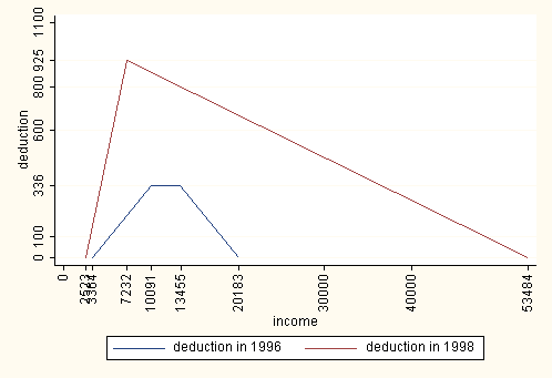
Figure 1. Earned income deduction

Source:Laine and Uusitalo 2001; Kurjenoja 2000

6.2
The increase in the amount of earned income deduction generally improves the attractiveness of working compared to social security. It must be noticed, however, that in 1998 the maximum amount of earned income deduction was 925 Euros when the amount of earned income was 7232 Euros/year. The national income tax-scale did not yet extend to this amount of income and meant that the total tax rate was about 20% (municipal taxation + compulsory insurance contributions). The real effect of the earned income deduction for those earning 7232 Euros/year was around 17 Euros/month (Laine and Uusitalo 2001).

Table 7: Tax rates in 1996 and 1998

Taxable earned income, in EurosTax at the lowest level, in EurosTax at the amount exceeding the lowest level, %
1996
7232-992387
9923-1227819717
12278-1749259721
17492-27415169227
27415-48774437133
48774-1142039

1998
7737-1042886
10428-1311917016
13119-1850160020
18501-29097167726
29097-51466443232
51466-1159038

Source: Finnish Tax laws 1998; Laine and Uusitalo 2001

6.3
The changes in the tax rate and the progressivity of taxation are presented in Table 7. The marginal tax rates were lowered at all income levels in 1997 and in 1998. The simulations of Laine and Uusitalo (2001) concentrated on marginal tax rates (income trap) and showed that the changes in both, the earned income deduction and in the tax scale dropped the marginal tax rates by approximately 2% for all income earners and after tax net wages increased on average 3-4% for all earning over 6728 Euros/year. Thus, the aggregate tax reforms did slightly encourage working even when the effect was not very great.

Day-care payments and home care subsidy

Day-care payments

6.4
All children under school age are entitled to communal day-care in Finland. In 1996 the number of family members and a cost-category of district of residence determined income limits on the bases of which the maximum payment of communal day-care was divided into five classes (see Table 8). If a family had more than one child eligible for day-care the payment of the youngest child followed the payment classes. For older siblings the payment class was one class below the class the younger child was in. It has been criticized that the payment classes created income traps for families with small children. Another criticism was that the payments varied considerably between districts/towns.

6.5
At the beginning of 1997 day-care payment classes were replaced by percentage based payments, which were the same in the whole country (see Table 9). The payment was dependent on family size and was proportional to the family's income. As an example, in a family of 1-2 members the payment was 11.5% of the amount exceeding the income limit of 866 Euros/month. The maximum payment/child was fixed at 168 Euros/month (Laine and Uusitalo 2001; Prime Minister's Office 1996; Niinivaara 1999; Kurjenoja 2000). Laine and Uusitalo (2001) report that the reform of the day-care payments eliminated over 100% effective marginal tax rates and lowered some of the income traps that existed in 1996.

Table 8: Communal day-care payments in 1996 in Helsinki, Euros/month

Income limits of the day-care payments
Size of the family12345
29921446156416992641
312611766191721023330
415472220238826074121
518842557280931124928

Source: Kurjenoja 2000

Table 9: Communal day-care payments in 1997 (whole country), Euros/month

Size of the familyMinimum income limitPercentage of deduction
1-286611.5
310689.4
412687.9

Source: Kurjenoja 2000
Home care subsidy

6.6
Home care subsidy is paid to families with a child or children under 3 years of age who are not attending communal day-care. The allowance is paid after the end of the parent allowance period, which is 158 days. In 1996 home care subsidy consisted of the basic component, 252 Euros/month, sibling supplement, 51 Euros/month/child and an earnings-related additional component (see Table 10). The basic component was allowed to all those entitled to the allowance. The sibling supplement was given to all children in the same family under 7 years of age and not attending the municipal day-care. The earnings-related component required that the family's income did not exceed a predetermined limit (see Figure 2). The limit in 1996 was 777 Euros/month. If the family's income was more than this limit, the full earnings-related component (202 Euros/month) was cut by 15% of the amount above the limit. The earnings-related supplement was not paid if the family's income exceeded 2119 Euros/month (Kosunen 1997; Laine and Uusitalo 2001; Prime Minister's Office 1996; Varma 1996).

Table 10: Home care subsidy in 1996 and 1997, Euros/month

Basic amountSiblings supplement
Earnings-related compnent
Year 199625251202
Year 1997Care benefit
252/84/51
Care allowance
168

Source: Kosunen 1997; Laine and Uusitalo 2001; Prime Minister's Office 1996; Varma 1996

Table 11: Determination of care allowance in 1997, Euros/month

Size of the familyIncome limitPercentage of deduction
2115911.5
314269.4
416947.9

Source: Kosunen 1997; Laine and Uusitalo 2001; Prime Minister's Office 1996; Varma 1996

6.7
In 1997 the whole system of home care subsidy was renewed and private care assistance was introduced. Parents could choose between communal day-care, home care subsidy or private care assistance for children under 3 years of age and between communal day-care and private care assistance for children under school age. Both home care subsidy and private care assistance included care benefit and an earnings-related care allowance (see Table 11). Care benefit was 252 Euros/month for the first child, 84 Euros/month for the second child and 51 Euros/month for all other children under school age. In 1997 the amount of care allowance depended not only on the family's income but also on the size of the family (see Table 11 and Figure 2). For a two-member family the income limit was 1159 Euros/month and the percentage for deduction was 11.5% for the amount exceeding the income limit.

Figure
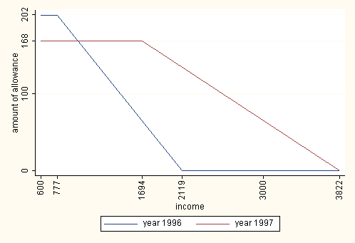
Figure 2. Earnings related component of home care subsidy in 1996 and earnings related care allowance in 1997 for four member family

Source:Kurjenoja 2000; Varma 1996; Varma 1997; Laine and Uusitalo 2001

6.8
For a three-member family the corresponding figures were 1426 Euros/month with a 9.4% deduction and for a family with four members 1694 Euros/month and a 7.9% deduction. The full amount of care allowance was 168 Euros/month (Kosunen 1997; Laine and Uusitalo 2001; Prime Minister's Office 1996; Varma 1996; Varma 1997; Kurjenoja 2000).

6.9
For a two-adult family with two children of day-care age, the reform increased the amount of home care subsidy when one of the spouses was working and the other one took care of the household, and the income of working spouse was between 1009 and 3818 Euros/month. The increased amount of the home care subsidy resulted in worse work incentives for the spouse taking care of the household. With family income less than 1009 Euros/month the reform cut the amount of home care subsidy, which mean that the incentives to receive work outside the household increased. In brief, the home care subsidy reform decreased the labor supply of parents with small children. The total effect on the labor supply, however, also depends on the reform of day-care payments (Laine and Uusitalo 2001).

Housing allowance and social assistance

Housing allowance

6.10
Low income households are eligible to receive housing allowance for both owner-occupied housing and for rented accommodations. Housing allowance is means-tested where housing expenditure, household total income and taxable income (including wealth) all affect the net amount of the allowance. In 1996 the amount of housing allowance was 80% of the reasonable housing expenditure which exceeded the excess expenditure. The excess amount was determined by the number of individuals living in a household, by the household income and by the location of the residence. The reforms implemented in 1998 increased the amount of housing allowance to cover at least the total range of social assistance. This meant that the income limit was extended for those living alone to an equivalent level with unemployment assistance and for other households to an equivalent level of housing allowance in 1995. Furthermore, the 17 Euros excess was removed (Varma 1996; Varma 1998; Laine and Uusitalo 2001; Prime Minister's Office 1996; Niinivaara 1999).

6.11
An individual whose own income (added to the income and assets of other members of the same household) is not enough to provide an adequate level of livelihood is eligible for social assistance. The amount of assistance is means-tested based on household disposable income and those expenditures entitled to this assistance. Social assistance is formed by the basic amount and by the amount which is separately defined. In 1996 the effective marginal tax was 100% for a household receiving social assistance because earned income cut the assistance by the full amount. The social assistance was changed in 1998 so that it now included 7% excess amount of housing costs (Varma 1996; Varma 1998; Laine and Uusitalo 2001; Prime Minister's Office 1996; Niinivaara 1999).

6.12
For incomes lower than 505 Euros/month the reforms (both housing allowance and social assistance) had almost no effect. The main effect of the combined reform was a decline in reservation wages due mainly to the rise in the income limits of the housing allowance. Increase in earned income raised the amount of disposable income already at the level of 488 Euros income/month. The reservation wage under the old system was 622 Euros/month. The 100% marginal tax rates, resulting from social assistance, had an effect after the reform only at the income level of less than 488 Euros/month. The biggest effect results from the increased level of housing allowance (increased income limits) (Laine and Uusitalo 2001; Niinivaara 1999).

Unemployment benefit

6.13
The unemployment benefit is formed by two main benefit categories: the unemployment allowance and labor market support which was introduced in 1994. The unemployment allowance is divided again into two categories: the earnings-related daily allowance and the basic daily allowance. If a person is partly unemployed, for example in cases of temporary dismissal or part-time work, she/he is eligible for adjusted allowance, meaning that part of the earned income is deducted from the original amount of unemployment allowance during the period of adjustment. The unemployment allowance was cut in 1996 by 80% of the earned salary and in 1997 the same cut was 50%. This meant that every earned euro after 1997 cut the allowance by 50 cents. The intention of the reform was to reduce the income dependence of unemployment allowance and the purpose was to make working profitable even when receiving this allowance.
Labor market support

6.14
Labor market support is a means-tested benefit where not only the individual's own income but also the earned income of a spouse exceeding 51 Euros/month affect the final amount of the support. In 1996 the income limit of labor market support was 933 Euros/month for an individual with children and 622 Euros/month for an individual with no children. Benefit was extended by 106 Euros/month for every child under 18 years of age. Labor market support was cut by 75% of the income exceeding the income limit. In 1997 the conditions of the benefit were changed so that the new income limit for a couple, married or cohabiting, was now 848 Euros/month and the labor market support was cut by 50% of the income exceeding the limit. For an individual with no children the income limit dropped to 252 Euros/month and the reduction remained at the level of 75%. Other conditions remained unaltered (Varma 1996; Varma 1997; Varma 1998; Laine and Uusitalo 2001; Prime Minister's Office 1996).

6.15
The reform increased the amount of labor market support for most of the unemployed and thus made working less attractive than before for the spouse not working. The reform also affected the incentives of a working spouse. As an example, by lowering the means-test prerequisites of the benefit, the marginal effective tax rates decreased for the working spouse when the salary was between 1177 and 1850. At this income level, the work incentives increased and due to the substitution effect the labor supply should increase as well. According to the empirical results of Laine and Uusitalo (2001) the labor supply of the working spouse increased as a result of the reform.

* Notes

1 For more information about the changes in income inequality and poverty in Finland in the 1990s see Mattila-Wiro (2006).

2 The GE(2), half the squared coefficient of variation, belongs to the family of Generalized Entropy inequality indices. They have a property of being only indices that are additively decomposable by population subgroups, and several members can also be decomposed by income sources. Thus, they are very useful measures in studying the level, the trend and the structure of inequality. The GE(2) can have values ranging from 0 to infinity. Zero represents an equal distribution (all incomes identical) and higher values represent higher levels of inequality (see for exampleLitchfield 1999).

3 The Gini coefficient, or the relative mean difference, is a very direct measure of income inequality that takes note of differences between every pair of incomes. The Gini coefficient belongs to the summary measures of concentration and it describes the extent of inequality. It is usually viewed by using the Lorenz curve. The Lorenz curve is a graph of cumulative income shares against cumulative population shares. The Gini coefficient is the ratio of the difference between the diagonal, the absoluteequity, and the Lorenz curve to the triangular region underneath the diagonal (Foster and Sen 1997). The Gini coefficient ranges from a maximum of 1, which depicts perfect inequality, to 0, which depicts perfect equity.

4 The comment of the Referee is gratefully acknowledged.

5 The comment of a Referee is gratefully acknowledged.

6 The advantage of the method used is that the income transfers now describe all the transfers received by individuals in each cell weighted by the share of recipients of each transfer. Then alternative earnings do not have to be calculated separately for each income transfer. Furthermore, the expected net wage for those not working is acquired, which is an average wage for those of the same age, having similar education and being in a similar family situation (Laine and Uusitalo 2001).

7 The OLS regression was used to cell-mean data.


* References

AARBU, K. O. and Thoresen, T. O. (1997), The Norwegian Tax Reform; Distributional Effects and the High-income Response, Discussion Paper 207, Statistics Norway, Research Department, Oslo.

BLUNDELL, R., Duncan, A. and Meghir, C. (1998), 'Estimating labor supply responses using tax reforms', Econometrica 66(4), 827-861.

DUNCAN, A. and MacCrae, J. (1999), Household Labour Supply, Childcare Costs and In-Work Benefits: modelling the impact of the Working Families Tax Credit in the U.K. Paper presented to the Econometric Society European Meeting.

FINNISH Tax Laws (1998), Helsinki. In Finnish.

HEIKKILÄ, M. (1997), Justifications for cutbacks in the area of social policy, in 'The Cost of Cuts. Studies on cutbacks in social security and their effects in the Finland of the 1990s', STAKES, National Research and Development Centre for Welfare and Health, Helsinki, pp. 15-28.

HEIKKILÄ, M. and Uusitalo, H., eds (1997), The Cost of Cuts. Studies on cutbacks in social security and their effects in the Finland of the 1990s, number 208 in 'Reports', STAKES, National Research and Development Centre for Welfare and Health, Helsinki.

KOSUNEN, V. (1997), The recession and changes in social security in the 1990s, in M. Heikkilä H. Uusitalo, eds, 'The Cost of Cuts. Studies in cutbacks of social security and their effects in the Finland of the 1990s.', STAKES, National Research and Development Centre for Welfare and Health, Helsinki, pp. 41-68.

KURJENOJA, J. (2000), Income taxation as a medicine to incentive traps, Tax information 24, Central Association of Taxpayers, Helsinki. In Finnish.

KURJENOJA, J. (2004), For whom is the work worth while?, Tax information 39, Central Association of Taxpayers, Helsinki. In Finnish.

LAINE, V. and Uusitalo, R. (2001), Labour supply effects of the Finnish work incentives reform, Research 74, VATT, Government Institute for Economic Research, Helsinki. In Finnish.

LITCHFIELD, J. A. (1999), Inequality: Methods and Tools, STICERD, Suntory and Toyota International Centres of Economics and Related Disciplines, London School of Economics, London.

MATTILA-WIRO, P. (2006), Changes in the Distribution of Economic Wellbeing in Finland, VATT Research Reports 128, Helsinki.

NIINIVAARA, R. (1999), The assessment of the impementation of the proposals made by the Incentive Trap Task Force, Research 4/99, Ministry of Finance, Helsinki. In Finnish.

PRIME MINISTER'S OFFICE (1996), The final report of the Incentive Trap Task Force, Publications 5, Prime Minister's Office, Helsinki. In Finnish.

FOSTER, E. F. and Sen, A. (1997), On Economic Inequality, Oxford University Press, Oxford, Edition 2.

STATISTICS FINLAND (2003), Income distribution statistics 2001, Income and Consumption 13, Helsinki. In Finnish.

UUSITALO, H. (1997), Four years of recession: What happened to income distribution? , in M. Heikkilä H. Uusitalo, eds, 'The Cost of Cuts. Studies on cutbacks in social security and their effects in the Finland of the 1990s', STAKES, National Research and Development Centre for Welfare and Health, Helsinki, pp. 101-118.

VARMA (1996), Livelihood security 1996, Technical report. In Finnish.

VARMA (1997), Livelihood security 1997, Technical report. In Finnish.

VARMA (1998), Livelihood security 1998, Technical report. In Finnish.

----

ButtonReturn to Contents of this issue