Heiko Rauhut and Marcel Junker (2009)

Punishment Deters Crime Because Humans Are Bounded in Their Strategic Decision-Making

Journal of Artificial Societies and Social Simulation 12 (3) 1
<https://www.jasss.org/12/3/1.html>

For information about citing this article, click here

Received: 22-Dec-2008    Accepted: 16-May-2009    Published: 30-Jun-2009

Abstract

Is it rational to reduce criminal activities if punishments are increased? While intuition might suggest so, game theory concludes differently. From the game theoretical perspective, inspectors anticipate the effect of increased punishments on criminal behavior and reduce their inspection activities accordingly. This implies that higher punishments reduce inspections and do not affect crime rates. We present two laboratory experiments, which challenge this perspective by demonstrating that both, criminals and inspectors, are affected by punishment levels. Thereupon, we investigate with agent-based simulations, whether models of bounded rationality can explain our empirical data. We differentiate between two kinds of bounded rationality; the first considers bounded learning from social interaction, the second bounded decision-making. Our results suggest that humans show both kinds of bounded rationality in the strategic situation of crime, control and punishment. We conclude that it is not the rationality but the bounded rationality in humans that makes punishment effective.

Keywords:

Crime, Punishment, Control, Bounded Rationality, Agent-Based Simulation, Experiment, Game Theory

Introduction

1.1

It seems straightforward that higher punishments deter crime. Early thinkers, as Cesare Beccaria, outlined this idea and it was first formalized by Gary Becker (Becker 1968). In the meanwhile, it is known as the "economic model of crime" or as the rational-choice theory of crime. Its main assumption states that criminals are rational. A thief is a thief and a professor is a professor because these professions make both better off given their individual alternatives, preferences and restrictions. If we modify the criminals' restrictions, i.e. if we increase punishment, crime will become less attractive and, therefore, the crime rate will decrease. However, the empirical literature fails to find consistent effects of punishment on crime. A recent extensive overview summarizes these findings trenchantly in the title: "Sentence severity and crime: Accepting the null hypothesis" (Doob and Webster 2003).

1.2

Game theory offers an explanation why punishment does not deter crime. The game theoretical argument states that the social interaction between criminals and inspectors, like police officers or public prosecutors, causes a paradoxical aggregation of the behavior of both players. This aggregation of strategic reasoning shifts the effect of severity of punishment from the criminals' to the inspectors' behavior. The underlying mechanism is the game theoretical concept of mixed Nash equilibria, which requires rational agents to outsmart their opponents. This model assumes that criminals choose the probability of committing a crime at the indifference point of the inspectors, and inspectors choose the probability of inspection at the indifference point of the criminals (Tsebelis 1989; Tsebelis 1990; Rauhut 2009). Thus, higher punishment does not reduce criminal activities, but it reduces inspection activities. In this article, we investigate with laboratory experiments and tailor-made simulation models whether humans apply sufficient strategic reasoning so that the game theoretic mechanism holds.

A game theoretical model of crime and punishment

2.1

Let us first consider the economic model of crime as a theoretical foundation of the game theoretic model. The economic model of crime assumes that criminals are utility maximizers who optimize their payoffs under restrictions and risk (Becker 1968). The payoffs consist of material gains in the case of theft or burglaries, or in immaterial, psychic gains in the case of assaults. The restrictions for criminal behavior consist of punishment threats. The risk is given by the probability of being caught and to become subject to punishment. More specifically, let criminal i receive the combined monetary and psychic payoff g for a certain criminal behavior. Let her face the detection probability c to receive the punishment costs p. Let s_i denote the likelihood that criminal i commits the crime. Thus, we can write the payoff function of criminal i as

πi ( si ) = si ( g–c p ) .

(1)

2.2

We can see from equation (1) that higher punishment reduces criminal activities. However, Becker's analysis neglects strategic interaction. The detection probability c is not an external factor, but it is determined by the decisions of the activities of police officers, public prosecutors or lawyers (Tsebelis 1989; Rauhut 2009). We can assume that these actors decide as well according to rationality considerations. More specifically, criminals and inspectors are in a so-called "discoordination game". Criminals prefer to commit a crime if they can be sure that they will be not detected and punished. In contrast, inspectors prefer to inspect the criminals if they are sure that they will detect the crimes of the criminals.

2.3

To understand the strategic situation between criminals and inspectors more intuitively, let us consider two examples of discoordination situations from sports. In the case of penalty kicks in soccer (Chiappori et al. 2002), the goalkeeper prefers to dive left when the penalty kick goes left and prefers the right side if the kick goes right. In contrast, the kicker will shoot left if she assumes that the goal-keeper will dive right, and vice-versa. A similar situation is found in tennis, where the serving player aims to outplay the returning player. It is best to serve longline when the return player expects a cross and vice versa (Walker and Wooders 2001). In both examples, one player is interested in a match, and the other player is interested in a mismatch, because the gain of one player is the loss of the other. The only rational choice is to play a probability mixture of the strategies. Only if both players calibrate their probability mixtures such that their respective opponent is indifferent between her alternatives, the combination of both probability mixtures will be stable. Indifference means that a player has no possibility to increase her outcome by changing her probability mixture.

2.4

In the game theoretic model of crime (Tsebelis 1989; Rauhut 2009), criminals and inspectors are assumed to be in a similar discoordination situation as soccer or tennis players. As the criminals are inspected, we call them inspectees. Inspectees can decide to commit a crime or not with similar payoffs as given in equation (1). Inspectors can decide to invest in inspection costs k to inspect the inspectee. If the inspector detects a crime, she receives the reward r, while the inspectee receives her punishment p. This "inspection game" can be illustrated with the 2×2 matrix in Table 1.

Table 1: The inspection game. Payoffs for inspectees are given on the left and for inspectors on the right side of the comma. The payoffs denote: g gains for crime, p punishment, k inspection cost, r rewards for successful inspection with p > g > 0, r > k > 0.
			Inspector j
		inspect		not inspect
Inspectee i	crime	g–p , r - k	⇐	g , 0
		⇓		⇑
	no crime	0 , -k	⇒	0 , 0

2.5

There is no solution in pure strategies due to p > g > 0 and r > k > 0. Therefore, actors have to choose the particular probability mixture of their strategies which leaves their opponent indifferent. If both players are not indifferent, one player can exploit the other, which provides an incentive for the latter to change her strategy. Let, according to s_i, denote c_j the probability mixture to inspect. We acknowledge the additional second player, the inspector, with an extension of the payoff function of the economic model of crime (equation 1). Thus, the payoff function π for inspectee i who plays against inspector j is now given by

πi ( si , cj ) = si ( g–cj p ) .

(2)

2.6

The payoff function φ for inspector j who plays against inspectee i is

φj ( si , cj ) = cj ( si r–k ) .

(3)

2.7

We obtain the particular Nash equilibrium of the probability mixture of inspectee i which makes her opposing inspector j indifferent, if we calculate the first partial derivative of the inspectors' payoff function δφ_j/δc_j and set it zero. Thus, inspectee i chooses the probability of committing a crime as

si* = k/r .

(4)

2.8

Likewise, we obtain the probability mixture of inspector j which makes her opposing inspectee indifferent by calculating the first partial derivative of the inspectees' payoff function δπ_i/δs_i and set it zero. As a result, inspector j chooses the probability of inspection as

cj* = g/p .

(5)

2.9

Results are counterintuitive: Higher punishment does not reduce crime, but it reduces inspection behavior. Nevertheless, we can make sense of this result, if we recall our examples from sports. In situations with entirely opposing interests, it is reasonable to base our decision-making on the payoffs of our opponent instead of our own payoffs.^[1]

2.10

While the model might be a realistic model of crime and punishment for entirely rational individuals, we might ask ourselves, whether humans' rationality holds for such sophisticated strategic reasoning. In particular, one might question the plausibility that actors know their opponents' payoffs and that actors are sufficiently smart to react optimally on their opponents' payoffs in calibrating their strategy mixture exactly at the indifference point of their opponent.

2.11

In the following, we present two laboratory experiments to test the predictions of Nash equilibria in mixed strategies. We collect laboratory data instead of field data because this allows to measure causal effects with higher internal validity and to conduct more in-depth investigations of the underlying mechanisms. Furthermore, the achievement of high internal validity is crucial as some of the former field studies do not find punishment effects (Sherman 1993; MacCoun and Reuter 1998; Doob and Webster 2003), while others do (Cameron 1988; Levitt 1997; Nagin 1998). Moreover, there are almost no laboratory experiments on strategic interaction in the field of crime and punishment, except Falk and Fischbacher (2002) and Rauhut (2009). After a statistical analysis, we compare our empirical results with tailor-made simulation models of bounded rationality to draw inferences on the level of bounded rationality in humans in the area of crime and punishment.

Empirical evidence from two laboratory experiments

Implementation of the abstract inspection game in the laboratory

3.1

We extend the original inspection game given in table 1 to enhance the construct validity of crime and inspection in our empirical test. Also we aspire that our subjects recognize the abstract situation in the laboratory as being similar to the strategic interaction between potentially criminal citizens and police officers. Our solution is to implement real theft behavior between the inspectees. Therefore we extend our game from two to four players: Two inspectees, who can both steal money from each other, and two inspectors, each allocated exclusively to one inspectee (see figure 1). The allocation of one inspector to one inspectee guarantees equal statistical power for inspectees and inspectors in our statistical tests.

3.2

Inspectees who perpetrate their matched inspectee enjoy a criminal gain of g while their victim suffers a loss of l. Due to g < l, mutual theft produces a welfare loss among both inspectees, representing the collective inefficiency of most criminal activities. Without inspectors, the dominant choice were to commit a theft. However, both inspectors can decide to inspect her inspectee and reveal her decision. In the case that the inspected inspectee committed a theft, the inspector receives her reward r, with r > k, and the inspectee receives her punishment p. It can easily be shown that the Nash equilibria in mixed strategies of the simpler model, given in equations (4) and (5), are similar to the extended game. Formally, inspectee i can be inspected by inspector j and victimized by inspectee h, so that her utility function is given by

πi ( si , sh , cj , cl ) = si ( g–cj p )–sh l .

(6)

3.3

Likewise, the utility function φ for inspector j who can inspect inspectee i is given by

φj ( si , sh , cj , cl ) = cj ( si r–k ) .

(7)

3.4

Rearrangement and calculation of the partial derivatives yields the equilibrium in mixed strategies of crime as s_i* = k/r and of inspection as c_j* = g/p. Therefore, our previous predictions remain similar for our experimental design that higher punishment should not deter crime but inspection.

Experimental parameters and procedure

3.5

The experiment is conducted in a computer laboratory at the University of Leipzig and programmed with the software z-Tree (Fischbacher 2007). Subjects interact anonymously via a computer network. In the first part of the experiment, subjects earn own property by giving correct answers in a knowledge quiz. Then, subjects are randomly split into inspectees and inspectors and keep their role for all 30 periods of the experiment. In each period, inspectees and inspectors are randomly assigned into groups of four-two inspectees and two inspectors. One inspectee can steal money from the other inspectee's account and vice versa. For each inspectee, there is one inspector who can decide to invest inspection costs to uncover the action of the inspectee and obtain rewards for detected crime. A visualization is given in figure 1.

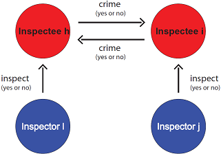
Figure 1. The design for measuring crime and punishment in the laboratory experiment and in the agent based simulation

3.6

Subjects are given the following information after each period. Inspectee i learns the decision of her matched inspectee h and the decision of her matched inspector j and, if eligible, whether she has been punished. Inspector j learns the decision of her matched inspectee i. Players learn their current income level each period. Note, however, that subjects only learn the decisions of the players they are matched with and not the decisions from the other participants in the session.

3.7

The monetary payoffs for the subjects are presented in experimental points and later transferred into money. Subjects receive g/p = 5/6 points in the low punishment regimes and g/p = 5/25 in the high punishment regimes. We keep inspection rewards constant in all sessions at k/r = 5/10 points. Our implementation considers the above mentioned criminal dilemma because victims of theft suffer l = 10 losses, while criminals gain only half of this damage (g = 5). The payoffs are transferred to Euro such that inspectees start in average with 22 Euros and loose 16 Euros due to theft, while inspectors stay at around 4.50 Euros (for final incomes, add 5 Euros show up fee).

3.8

Our experimental design follows a 2×2 design to test punishment effects on crime and inspection irrespective of timing effects. To control for such timing effects, experiment 1 implements 15 crime and 15 inspection decisions for low punishment and compares it with subsequent 15 crime and 15 inspection decisions for high punishment. In experiment 2, the reversed order is realized. 20 subjects take part in 10 separate experimental sessions; except session 3 with 16 subjects. In total, our generalizations rely on N = 196 subjects and n = 5880 decisions.

Statistical analysis of the empirical data

3.9

In a first step, we concentrate our statistical analysis on a visual impression of the main characteristics of our data. Figure 2 displays box-plots of the mean crime and inspection rates in percentages. For producing the box-plots, we calculated the average crime and inspection rate in each period, separately for experiment 1 and 2 and separately for low and for high punishment conditions. These calculations return 15 crime and 15 inspection rates for each of the 4 conditions (2 experiments × 2 levels of punishment). The 4 box-plots represent the distribution of these crime and inspection rates in all 4 conditions. Note that the underlying crime and inspection decisions are dichotomous (yes or no). The distribution in each box is based on 50 subjects (50 inspectees and 50 inspectors for each of the two experiments; note however that our data consists of 196 instead of 200 subjects).

3.10

Our empirical evidence shows two interesting results: Firstly, higher punishment deters inspection, but compared to the Nash predictions, inspection rates are too insensitive for punishment levels. We expect with eq. (5) and with the chosen experimental payoffs an inspection rate of 20% for high punishment and of 83% for low punishment. Secondly, higher punishment deters crime, too, so that crime rates are too sensitive for punishment. We expect from eq. (4) with the chosen payoffs constant crime rates of 50% for both punishment levels.

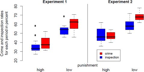
Figure 2. Higher punishment deters crime and inspection. In experiment 1, punishment is increased from 15 periods low punishment to 15 periods high punishment. Experiment 2 implements the reversed order. Red boxplots represent crime rates for 15 periods of low punishment vs. 15 periods of high punishment, blue boxplots represent corresponding inspection rates. For entirely rational humans, higher punishment would only reduce inspection activities and leave crime rates constant. Mixed Nash equilibria from game theory predict inspection rates at 20% for high punishment and at 83% for low punishment. Crime rates are predicted to be constant at 50% for both punishment levels. A comparison of empirical data with Nash predictions reveals that, in high punishment regimes, too high inspection rates match too low crime rates and, in low punishment regimes, too low inspection rates match too high crime rates. Such synchronized patterns suggest strategic interaction of humans with bounded rationality.

3.11

In addition, figure 2 highlights the value of strategic analyses of crime and punishment because crime and inspection rates follow synchronous patterns. Inspectees and inspectors coordinate their behavior strongly despite they do not meet theoretical predictions exactly. For high punishment, we observe too much inspection and therefore too little crime. For low punishment we observe too little inspection and therefore too much crime. Such empirical patterns suggest that humans follow rational criteria in strategic and individual decision-making on one hand but show rationality flaws on the other hand, which hinder optimal choices.

3.12

Subsequently, we analyze whether our findings are statistically significant. The data consists of dichotomous decisions; inspectees decide to commit a crime or not and inspectors decide to perform control or not. We employ logistic regression models to estimate the change in the probability of committing a crime respectively performing control for the two different levels of punishment. In addition, we have to take the clustering of our data into account. Each subject meets 30 decisions, because the low and the high punishment treatment consist of 15 periods each. We can account for the correlated decisions within subjects by estimating either logistic regressions with robust standard errors or logistic random intercepts models. Both methods yielded essentially similar results. We report only the random intercepts models in this article because they are more explicit in illustrating the strength of the clustering of the subjects' decisions.

Table 2: Logistic random intercepts models, illustrating the statistical significance of punishment effects on crime and inspection. Standard errors in parentheses, 2940 decisions clustered in 98 subjects. High punish: Dummy, 0-low, 1-high punishment. * p < 0.05, ** p < 0.01, *** p < 0.001.
	(1) Crime	(2) Inspection
Fixed effects
High punishment	-1.06*** (0.085)	-0.72*** (0.084)
Intercept	0.70*** (0.13)	0.28* (0.13)
Variance of Intercept	1.22 (0.23)	1.28 (0.24)
-2LogLikelihood	-1776.2	-1804.7
Bic	3576.4	3633.4
N (decisions)	2940	2940

3.13

Table 2 shows the results of the random intercepts models for the effects of the strength of punishment on the probability to commit a crime and to perform control. Our analyses rely on 2940 decisions, clustered in 98 inspectees and 98 inspectors. Higher punishment has a highly significant negative effect on both, criminal and inspection behavior. Our descriptive results of the box-plots can therefore be substantiated. Moreover, the coefficients suggest that the severity of punishment has a stronger effect on crime than on inspection behavior. The random part of the model reveals that the subjects' decisions are significantly clustered. The variances of the intercepts of criminal and inspection behavior are comparably large (1.22 and 1.28), and associated with comparably small standard errors. This strong clustering provides additional support for the generality of our conclusions, as the effects of punishment are highly significant despite the strong correlation within the subjects' decisions.

Understanding empirical anomalies with agent based simulations

Modeling bounded rationality

4.1

How can we explain discrepancies between theoretical models and empirical data? In the debate on crime and punishment, it is often argued if humans were entirely rational, punishment will have a strong impact on crime. Consequently, low correlations between crime and punishment are often explained with humans' lack of rationality (Pogarsky and Piquero 2003; Matsueda et al. 2006). But game theory uses rational, even "hyper-rational" assumptions, and concludes that entirely rational humans would not commit less crime with higher punishment threats. As a consequence, we propose the reverse argument. In our view, punishment deters crime only because humans are bounded in their rationality.

4.2

We can model human behavior as being prone to rationality flaws in processing information from social interaction or in a decreased capacity to maximize subjective utility. As a consequence, we develop two distinct models of bounded rationality. We call the first model Bounded Learning Model and the second Bounded Decision-Making Model. Bounded learning considers agents who are capable of meeting a correct decision but who are incapable to perceive their social environment correctly and to process information from social interaction adequately. Bounded decision-making considers additional factors in the decision-making, which can be described as random interferences on the decision process of the agents.

4.3

We derive subsequent predictions from agent-based simulations as the system becomes too complex for analytic solutions and because agent-based models can simulate artificial agents in a fictitious laboratory experiment. The agent-based simulations are strictly based on the experiment, such that the simulated agents play the same game as our human subjects. With variation in the agents' boundedness of rationality, the analysis of the simulated crime and inspection rates allows inferences on the boundedness of rationality in humans in situations of crime and punishment.

Two models of bounded rationality

4.4

We model bounded rationality by separating the agents' decision algorithms into two components. A rational component and a random component. In the Bounded Learning Model, we put random noise to the capability of agents to perceive their social environment correctly, in the Bounded Decision-Making Model, we put random noise to the agent's complete capability of meeting a rational decision. Note that bounded learning represents less rationality flaws than bounded decision-making. We incorporate the random component as the proportion ω, relative to the rational component. We vary ω between [0,1] to analyze punishment effects for increasing boundedness of rationality. We specify the random component η as a random draw from a uniform distribution.^[2]

4.5

In the Bounded Learning Model, inspectees' estimates of their subjective detection probability for criminal behavior is a compromise between a rational component c and a random component η. The rational component c is the perfect arithmetic mean of the subjectively experienced detection frequency. As the rational component c is a probability within the range [0,1], we specify the support of the uniform distribution between 0 and 1. Likewise, inspectors' estimates of the subjective detection probability is a compromise between a rational component s of the subjectively experienced detection frequency and a random component η, drawn from a uniform distribution between 0 and 1. Thus, inspectees commit a crime if their criminal gains outweigh their biased estimated detection probability times punishment, and inspectors inspect if their costs of inspection are outweighed by their biased estimated detection probability times their reward for successful inspection:

Inspectee i commits a crime if

g–(( 1 - ωi) ci + ωiη ) p > 0

(8)

Inspector j inspects if

(( 1 - ωj ) sj + ωjη ) r - k > 0

(9)

4.6

In the Bounded Decision-Making Model, inspectees' whole decision function is a compromise between a rational component and a random component. Inspectees commit a crime and inspectors inspect if their compromise between the rational component (g-cp respectively sr-k) and the random component η is positive. As agents meet dichotomous decisions, the subjective expected utility of agents can vary between -1 and 1. We draw η from a uniform distribution with a support between -1 and 1 with mean 0. We implement the following rules.

Inspectee i commits a crime if

( 1 - ωi ) (g–ci p) + ωiη > 0

(10)

Inspector j inspects if

( 1 - ωj ) ( sj r–k) + ωjη > 0

(11)

4.7

Note that we standardize payoffs in the Bounded Decision-Making Model with the biggest possible result to ensure results to be in the interval [-1,1], which is necessary for having comparable weights to the random term η. We are aware that the specific kind of noise drives the simulation results for both of our models. Nevertheless, a uniform distribution is in our opinion the most suitable and parsimonious implementation of random draws in this situation. Such random draws can be regarded as Null-hypothesis, implying as little information as possible.

Process of the agent-based simulation

4.8

We let the computer create n groups of four. As in our experiment, each group consists of two inspectees who can commit a crime on each other and two inspectors who can reveal the action of one inspectee. We initialize the simulation with a random draw for the belief about whether the opponent will commit a crime respectively perform a control. Each period of the simulation starts with a random match of inspectees and inspectors. In a second step, agents meet their decision, which is calculated by the respective decision-function and their subjective probability estimate of the choice of their opponent. Third, after each agent has met a decision, players learn the choice of their opponent. Lastly, inspectees update their estimate of the inspection rate with the arithmetic mean of their individually experienced inspection frequency and inspectors update their estimate of the crime rate with the arithmetic mean of their individually experienced frequency of crimes. Agents have a perfect memory of their experienced history and calculate perfectly the arithmetic mean from their experience. We repeat steps one to four for t time steps. Note that we drop the assumptions of "hyper-rationality" in game-theory: Agents do not know payoffs nor decision rules of their opponents. Furthermore, our agents are backward-looking instead of forward-looking as they react only on their experience instead of contemplating their opponent's choice in the future.

Analysis of the simulation and comparison with the empirical data

4.9

In a first step, we display single simulation runs. Figure 3 reports the crime and inspection rates averaged over all agents for simulations with a runtime of 1000 time steps each. We report results for low and high punishment scenarios, with the same payoffs used in the laboratory experiments. We differentiate the simulation charts for the two models of bounded rationality and for different degrees ω of bounded rationality in the agents (0%, 20%, 60% and 100% random). While figure 3 provides the dynamics of single runs, such as oscillations and mean behaviors, they likewise enable comparisons with the mixed Nash equilibria, which are represented by thinner blue and red lines. For the case of ω = 0, both models are identical and reproduce mixed Nash equilibria. Without bounded rationality, however, the oscillations are much larger compared to the situations with just little more random noise.

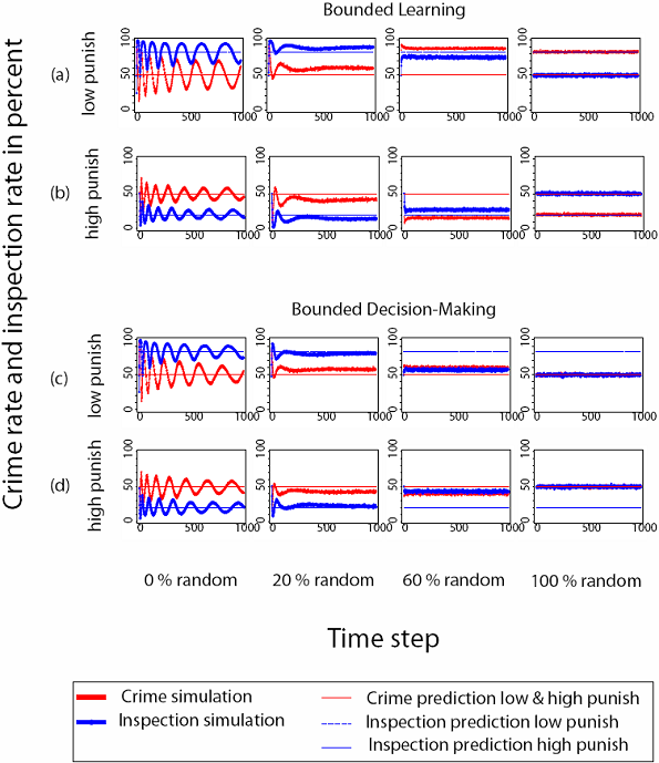
Figure 3. Comparison of simulated punishment effects on crime and inspection for different levels of bounded rationality. Each chart displays the dynamics of the crime and inspection rate over 1000 time steps in an exemplary simulation run with 1000 inspectees and 1000 inspectors. The four columns represent different levels of bounded rationality, expressed as the percentage ω of the random component η in the agents' decisions (0%, 20%, 60%, 100% random). The upper two rows (a) and (b) display results for modeling bounded rationality as "bounded learning" from social interaction. This bias consists of random noise in the agents' estimation of the detection probabilities for criminal behavior. In the lower two rows (c) and (d), bounded rationality is modeled as bounded decision-making. This "Bounded Decision-Making Model" considers different degrees of random noise ω for the whole decision function, producing gradually erratic behavior of the agents. Results for both models of bounded rationality can be compared for low punishment versus high punishment ((a) vs. (b) and (c) vs. (d)). Firstly, the results demonstrate that the mean of the oscillating crime and inspection rates approximate the theoretical prediction of the mixed Nash equilibria for the case of no random noise (ω = 0%) for both models. Secondly, the oscillations in the case of ω = 0% vanish rapidly for runs with greater ω. Thirdly, the mean crime and inspection rates are sensitive for different levels of bounded rationality ω. This sensitivity will be analyzed in greater detail and generality in Fig. 4

4.10

We analyze the sensitivity of the interaction between punishment strength, bounded rationality, crime and inspection in the agents in more detail and generality in figure 4. Here, theft and inspection rates are averaged over all agents and time steps. Each point represents an averaged simulation run, differentiated for different percent-values of ω and for bounded learning and bounded decision-making. Again, bounded learning and bounded decision-making reproduce game theoretic predictions if agents have no randomness in their decisions. If we subsequently increase ω and add random noise, punishment has an increasing impact on crime rates and a decreasing impact on inspection rates in both models. However, the complex interplay of social interaction is different in the models.

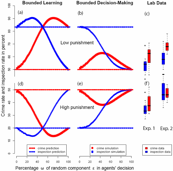
Figure 4. Punishment only deters crime if agents are bounded in their strategic decision-making. In the simulations ((a), (b), (c), (d)), each point represents the aggregated, average crime (red) and inspection rates (blue) over 1000 time steps and 1000 agents. (Single instead of aggregated runs can be seen in figure 3.) In the left "Bounded Learning Model", (a) and (d), agents are partially driven by random noise ω in estimating the detection probabilities of criminal behavior. In the "Bounded Decision-Making Model", (b) and (e), the complete decision function of the agents is biased by the random noise ω. The box-plots, (c) and (f), display the empirical inspection and crime rates from the two experiments described in chapter 2 and figure 2. Note for comparison that the crime and inspection data in the box-plots refer to the similar y-scale as the simulations. The upper part, (a), (b), (c), displays results for low punishment and the lower part, (d), (e), (f), for high punishment. Simulation results can be compared with Nash predictions, which are represented by dashed lines. For completely rational agents (ω = 0), both models reproduce Nash predictions: Higher punishment does not deter crime but exclusively inspection. Nash predictions do not hold for increasing ω. With an increasing lack of strategic reasoning, punishment has an increasing effect on crime and a decreasing effect on inspection. The two models predict different patterns of punishment effects and therewith enable comparisons with empirical data and inferences on rationality flaws in humans. The "Bounded Decision-Making Model" matches the empirical patterns (on the right side of the figure) well for a range of about ω ≈ 50%. This indicates that humans are both - bounded in their capacity to perceive their social environment correctly and in their capacity to maximize subjective utility.

4.11

Results for bounded learning show that increasing randomness pulls crime rates from inspectors' indifference point k/r to inspectees' own indifference point g/p. Likewise, it pulls inspection rates from g/p to 1–k/r. For this specific constellation, however, 1 - k/r equals k/r. More unambiguous cases can be seen in figure 5 with payoff combinations different from those in the lab experiment. We can conclude that with decreasing capability to process social information, game theoretic reasoning yields place to decision theoretic reasoning - for criminals, punishment levels become important and for inspectors, punishment levels become unimportant.

4.12

We can understand and interpret the results for bounded learning more clearly, if we consider the situation of maximum random noise with 100% random noise in the agents' decision function, which is expressed as ω = 1 in terms of our model variables. We can rewrite equations (8) and (9) as

Inspectee i commits a crime if

g/p > η

(12)

Inspector j inspects if

η > k/r

(13)

4.13

We can clearly see why the consideration of maximum noise shifts the equilibria from ego's indifference point to alter's indifference point. While the mixed strategy predicts that inspectees will choose the probability of committing a crime as k/r (inspection costs/inspection rewards), the Bounded Learning Model with 100% noise predicts the probability of committing a crime as g/p (criminal gains/punishment costs). This result holds for inspectors; except that they choose their reversed indifference point 1 - k/r (1 - (inspection costs/inspection rewards). For both types of agents for ω = 1, η is equal to their individual expectation value of crime respectively inspection. This implies that their probability is just guesswork, generated without using any knowledge or experience. As a consequence, agents meet their decision solely with respect to their own payoffs and disregard the payoffs of their opponents.

4.14

Results for the Bounded Decision-Making Model show that an increasing influence of randomness pulls equilibria for crime and control toward 50%. For low punishment, the compromise between the rational and the random component lets inspectees commit more crimes than predicted from Nash equilibria because inspection rates are below Nash equilibria. For high punishment, we observe the reverse order-too high inspection rates cause crime rates to stabilize at lower states than predicted by game theory.

4.15

Again, if we consider 100% noise, we can rewrite equations (10) and (11) as

Inspectee i commits a crime if

η > 0 .

(14)

Inspector j inspects if

η > 0 .

(15)

It is evident that the random variable η drives solely the decisions for committing crimes and for performing inspections.

4.16

A comparison between simulated and empirical data sheds light on the two kinds of bounded rationality in humans. The most typical empirical match of crime and inspection rates are their most often replicated patterns, illustrated with the 50% interquantile ranges in the boxes of the boxplots, shown in figure 2 and in small format in the subfigures 4c and 4f. For low punishment, crime rates between 54% and 66% coexist with inspection rates between 48% and 56% in experiment 1. In Experiment 2, crime rates between 64% and 72% coexist with inspection rates between 54% and 64%. There is no area in the Bounded Learning Model, where this would be true; either the differences between crime and inspection rates are higher or both rates are simultaneously higher. In the Bounded Decision-Making Model, the area ω ≈ 50% produces a pattern comparable to the empirical data. Likewise, we observe comparable patterns for high punishment. In experiment 1, crime rates between 33% and 46% coexist with inspection rates of 31% and 40%. In experiment 2, crime rates between 44% and 52% coexist with inspection rates between 42% and 56%. Again, there is no area in the Bounded Learning Model that matches this pattern, but the area around ω ≈ 50% randomness in the Bounded Decision-Making Model fits the data remarkably well.

Sensitivity analysis

5.1

We generalize and validate our findings by showing that simulation results hold for any payoff combination and not only for the payoff combinations used in the experimental design. We go through the parameter space of 5×5 payoff combinations, 5 for inspectees and 5 for inspectors. We select for g/p and for k/r payoffs of 0.05, 0.25, 0.5, 0.75, 0.95. Simultaneously, we go through the parameter space of levels of randomness ω in agents' decisions in 20 equally wide steps from 0 to 100 percent. Furthermore, we compute simulation values for both models, bounded learning and bounded decision-making. We set up simulations for 50 groups of four for 500 time steps. We summarize each simulation run with a certain payoff combination with its mean crime and mean inspection rate over all 500 time steps.

5.2

As the analysis is four-dimensional (crime/inspection rates over inspectees' payoffs over inspectors' payoffs over levels of randomness), we present results from two different perspectives; once, we fix payoff combinations and once randomness ω. First, we present with figures 5 and 6 two-dimensional scatter-plots. We show for fixed payoff combinations g/p and k/r the effect of the randomness ω in agents' decisions on the mean crime and inspection rates. Secondly, we present in three-dimensional contour-plots for fixed levels of randomness ω the effect of inspectees' and inspectors payoffs g/p and k/r on mean crime/inspection rates.

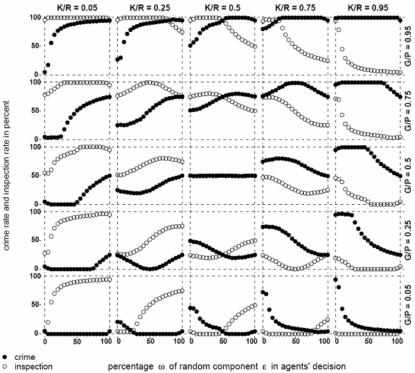
Figure 5. Bounded Learning: Effects of random noise ω on crime and inspection for fixed payoff combinations. K/R denotes inspectors' payoffs (inspection costs over inspection rewards k/r) and G/P denotes criminals' payoffs (criminal gains over punishment g/p). Points represent mean crime and inspection rates over 500 periods over 50 groups of four. The results confirm and generalize our previous simulations, which only covered analyses for the specific payoff combinations from the laboratory experiments: For minimal random noise ω, agents reproduce Nash equilibria for all payoff combinations: Crime rates increase for increasing K/R independently of G/P and inspection rates decrease for decreasing G/P independently of K/R. For maximal random noise ω, criminals' equilibria flip from opponents' indifference points k/r to their own indifference point g/p. Inspectors' equilibria flip from their opponents indifference point g/p to their reverse indifference point 1–k/r. Values in between minimal and maximal random noise ω produce equilibria between both scenarios.

Figure 6. Bounded Decision-Making: Effect of random noise ω on crime and inspection for fixed payoff combinations. K/R denotes inspectors' payoffs (inspection costs over inspection rewards k/r) and G/P denotes criminals' payoffs (criminal gains over punishment g/p.) Points represent mean crime and inspection rates over 500 periods over 50 groups of four. The results confirm and generalize our previous simulations, which only covered analyses for the specific payoff combinations from the laboratory experiment: For minimal random noise ω, agents reproduce Nash equilibria for all payoff combinations: Crime rates increase for increasing K/R independently of G/P and inspection rates decrease for decreasing G/P independently of K/R. With increasing random noise ω, agents equilibria for crime and inspection move toward 50%, which is the mean value of the uniform distribution we draw from to obtain our ω-values.

5.3

Figure 5 presents two-dimensional results for bounded learning and figure 6 for bounded decision-making. A comparison of the second and forth row for g/p for the middle column k/r = 0.5 is close to payoff conbinations in figure 4 so that we see comparable patterns. In general, for ω = 0, we replicate Nash equilibria, as crime rates equal inspection costs over inspection rewards k/r and inspection rates equal criminal gains over punishment g/p.

5.4

For bounded learning, increasing randomness ω sensitizes inspectees for punishment. For increasing ω, crime rates move from k/r to g/p. Equally, increasing ω makes inspectors sensitive for inspection rewards. As inspection rewards are positive incentives whereas punishments are negative incentives, effects for inspectors become reversed. For increasing ω, inspection rates move from g/p to 1–k/r.

5.5

Likewise for bounded decision-making, increasing randomness ω sensitizes inspectees for punishment and inspectors for inspection rewards. However, as randomness ω affects the whole decision function of agents, mean crime and inspection rates float for large values toward the mean of the uniform distribution, which is 0.5.

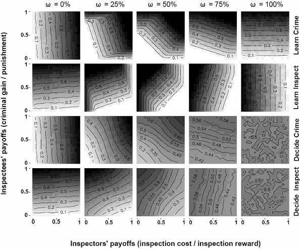
Figure 7. Three-dimensional contour plots: Effect of payoff combinations on crime and inspection for fixed levels of random noise ω. The contours show mean crime and inspection rates for simulation runs over 500 periods with 50 groups of four agents. Darker areas represent more crime respectively more inspection activities. Numbers in the contours represent 10% steps (e.g. 0.1 means 10%). The first two rows represent simulation runs for the Bounded Learning Model, with row 1 referring to the mean crime rate and row 2 to the mean inspection rate. Rows 3 and 4 represent simulation runs for the Bounded Decision-Making Model, with row 3 for crime and row 4 for inspection rates (e.g. Learn Crime refers to the mean crime rate for the Bounded Learning Model). Results confirm and generalize our previous restricted simulations for payoff combinations from the laboratory experiments. The first column of ω = 0 represents no random noise in both models, bounded learning and bounded decision-making. Here, crime rates only depend on inspectors' payoffs k/r as the vertical lines reveal. Inspection rates only depend on inspectees' payoffs g/p, as the horizontal lines reveal. For increasing randomness ω, crime rates depend increasingly on criminals' own payoffs so that the crime lines shift increasingly to horizontal positions. And inspection rates depend increasingly on inspectors' payoffs so that lines shift to vertical positions. In the Bounded Learning Model, increasing random noise ω forces crime and inspection rates to shift into complete randomness, which is in our model 50% crime and 50% inspection.

5.6

Figure 7 presents mean crime and inspection rates for the parameter space g/p × k/r for fixed values of ω = 0, 25, 50, 75, 100. The contours represent mean crime and mean inspection rates respectively. Darker areas represent more crime respectively more inspection activities.

5.7

In the Bounded Learning Model, for ω = 0, crime is only a function of inspectors' incentives k/r and inspection is only a function of inspectees' incentives g/p. Results flip for ω = 100: Crime is only a function of inspectees' incentives g/p and inspection is only a function of inspectors' incentives 1–k/r. In middle areas of ω =25, 50, 75, results are compromises between own and opponents' incentives. In the Bounded Decision-Making Model, crime and inspection rates do not flip entirely but float toward 50% for increasing ω.

5.8

In conclusion, our sensitivity analyses confirm the main results and support our conclusions from the simulation analysis of the parameter space used in the lab experiment.

Discussion

6.1

Our results suggest that humans are bounded rational in inspection situations. The results from our models suggest that humans are on the one hand bounded in their capacity to process accurately their information for meeting a rational decision, and, on the other hand, bounded in their ability to update correctly information from social interaction. We have demonstrated that bounded rationality provides a simple explanation for punishment effects on crime and inspection. Future research could explore the relative importance of both mechanisms in more detail.

6.2

Our findings highlight the complexity of punishment effects and twist the current debate on crime and punishment. First, punishment does not deter crime because humans are rational but because humans are bounded rational. Secondly, a change in punishment does not change criminal behavior but changes the interaction between criminals and inspectors.

6.3

Furthermore, our evidence relates to the current debate on so-called informal punishment. Informal punishment refers to punishment without material incentives and formal punishment to our case with material incentives. Current research demonstrated that actors are willing to punish non-cooperative players even in informal punishment regimes (Henrich and Boyd 2001; Sigmund et al. 2001; Fehr and Gächter 2002; Boyd et al. 2003; Fowler 2005; Gürerk et al. 2006; Rauhut and Krumpal 2008). Such behavior can be explained by relaxing the assumption of egoism in favor of fairness, or, in other terms, social preferences (Rabin 1993; Fehr and Schmidt 1999; Bolton and Ockenfels 2000). It is fascinating that the modification of both elements of the theory of rational action, egoism and rationality, improves the explanation of formal and informal punishment regimes. The relaxation of the assumption of egoism improves the explanation of informal punishment effects, and the relaxation of the assumption of rationality improves the explanation of formal punishment effects.

6.4

Prospective research might investigate more thoroughly the complex interplay of bounded rational agents. In particular, humans might be too slow to update previous beliefs so that they stick too firm to habits and irrational aspiration levels (Macy and Flache 2002). Additionally, humans might use wrong updating rules that cause otherwise unexpected punishment effects (Gigerenzer et al. 1996; Todd and Gigerenzer 2000). Further simulation studies might reveal the evolutionary path shaping human conditions in such a way that punishment mechanisms are effective to achieve cooperation for both kinds of punishment, with and without material incentives.

In memoriam

Very sadly, Marcel Junker lost his life only a few days before the publication of this article. With him, we are losing a very gifted, engaged and open-minded colleague and friend. The article at hand constitutes the first and only publication in his young career.

Acknowledgements

We gratefully acknowledge support from the DFG for financing experimental payoffs and research assistants (VO 684/5-1) and a research stay at the University of Michigan (VO 684/10-1). The manuscript benefitted from valuable comments made by Karl-Dieter Opp, Simon Gächter, Volker Grimm, Thomas Voss, Dirk Helbing, Dean Lacy, Florian Hartig, Michael Mäs, Roger Berger, Clemens Kroneberg, Mathias Franz and Tamara Münkemüller. The valuable research assistance from Isabel Kuroczka, Fabian Winter and Jana Adler is acknowledged.

Notes

¹One objection against the proposed game theoretic model might be that it is rather simplistic. More specifically, Bianco proposed in (Bianco et al. 1990) that the inspectee may make a deal with the inspector that she does not commit a crime if the inspector does not inspect. This deal can be of mutual advantage because it saves the punishment and the inspection costs compared to the strategy profile of probability mixtures, and it can be a pure Nash equilibrium if both actors interact repeatedly with each other. In this situation, higher punishments can reduce criminal activities because they reduce the minimum requirements of repeated interactions for such deals. In contrast, we argue, similar as Tsebelis in Bianco et al. (1990), that such voluntary agreements are rather unrealistic and only plausible in small towns with a limited number of police officers and inhabitants.

²Note that for the case of 0% both models are representations of the learning model "fictitious play" (Fudenberg and Kreps 1993; Fudenberg and Levine 1998). Nevertheless, our extension of the model fictitious play is new as we suggest two different extensions of the model (bounded learning and bounded decision-making). Both of these extensions measure bounded rationality with the percentage of random noise in the decision function. The difference between the models is the different component, which is subject to noise. As the focus of this article is on bounded rationality rather than on a systematic theoretical analysis and empirical validation of learning models, we do not pursue the analysis of learning models. However, the interested reader is referred to Rauhut (2009).

References

BECKER, G S (1968) Crime and Punishment: An Economic Approach. Journal of Political Economy, 76 (2), 169-217.

BIANCO, W T, Ordeshook, P C and Tsebelis, G (1990) Crime and punishment: Are one-shot, two person games enough?, American Political Science Review, 84, (2), 569-589.

BOLTON, G E and Ockenfels, A (2000) ERC: A Theory of Equity, Reciprocity, and Competition. American Economic Review, 90 (1), 166-193.

BOYD, R, Gintis, H, Bowles, S and Richerson, P J (2003) The evolution of altruistic punishment. Proc Natl Acad Sci USA, 100 (6), 3531-3535.

CAMERON, S (1988) The Economics of Deterrence: A Survey of Theory and Evidence. Kyklos, 41 (2), 301-323.

CHIAPPORI, PA, Levitt, S D and Groseclose, T (2002) Testing Mixed-Strategy Equilibria When Players Are Heterogenous: The Case of Penalty Kicks in Soccer. American Economic Review, 92, 1138-1151.

DOOB, A N. and Webster, C M (2003) Sentence Severity and Crime: Accepting the Null Hypothesis. Crime and Justice. A Review of Research, 28, 143-195.

FALK, A and Fischbacher, U (2002) Crime in the Lab. Detecting Social Interaction. European Economic Review, 46, 859-869.

FEHR, E and Schmidt, K M (1999) A theory of fairness, competition, and cooperation. Quarterly Journal of Economics, 114 (3), 817-868.

FEHR, E and Gächter, S (2002) Altruistic Punishment in Humans. Nature, 415 (10), 137-140.

FISCHBACHER, U (2007) Z-Tree. Zurich Toolbox for Ready-made Economic Experiments. Experimental Economics, 10 (2), 171-178.

FOWLER, J H, (2005) Altruistic punishment and the origin of cooperation. Proc Natl Acad Sci USA, 102 (19), 7047-7049.

FUDENBERG, D and Kreps, D M (1993) Learning Mixed Equilibria. Games And Economic Behavior, 5 (3), 320-367.

FUDENBERG, D and Levine, D K (1998) The Theory of Learning in Games. MIT Press, Cambridge, MA.

GIGERENZER, Gerd and Goldstein, D G (1996) Reasoning the fast and frugal way: Models of bounded rationality. Psychological Review, 103 (4), 650-669.

GÜRERK, Ö, Irlenbusch, B and Rockenbach, B (2006) The competitive advantage of sanctioning institutions. Science, 312 (5770), 108-111.

HENRICH, J and Boyd, R (2001) Why people punish defectors. Journal of Theoretical Biology, 208, 79-89.

LEVITT, S D (1997) Using electoral cycles in police hiring to estimate the effect of police on crime. American Economic Review, 87 (3), 270-290.

MACCOUN, R and Reuter, P (1998) Drug Control. In Michael Tonry (Ed.), The Handbook of Crime and Punishment, New York: Oxford University Press, 207-238.

MACY, M W and Flache, A (2002) Learning Dynamics in Social Dilemmas. Proc Natl Acad Sci USA, 99, 7229-7236.

MATSUEDA, R L, Kreager, D A and Huizinga, D (2006) Deterring Delinquents: A Rational Choice Model of Theft and Violence. American Sociological Review, 71, 95-122.

NAGIN, D S (1998) Criminal Deterrence Research at the Outset of the Twenty-First Century. Crime and Justice. A Review of Research, 23, 1-42.

POGARSKY, G and Piquero, A R (2003) Can Punishment Encourage Offending? Investigating the Resetting Effect. Journal of Research in Crime and Delinquency, 40 (1), 95-120.

RABIN, M (1993) Incorporating fairness into game theory and economics. American Economic Review, 83 (5), 1281-1302.

RAUHUT, H and Krumpal, I (2008) Enforcement of social norms in low-cost and high-cost situations. Zeitschrift für Soziologie, 5, 380-402.

RAUHUT, H (2009) Higher punishment, less control? Experimental evidence on the inspection game. Rationality and Society, 21 (3).

SHERMAN, L W (1993) Deffiance, Deterrence, and irrelevance: A theory of the criminal sanction. Journal of Research in Crime and Delinquency, 30 (4), 445-473.

SIGMUND, K, Hauert, C and Nowak, M A (2001) Reward and punishment. Proc Natl Acad Sci USA, 98 (19), 10757-10762.

TODD, PM and Gigerenzer, G (2000) Precis of Simple heuristics that make us smart. Behavioral And Brain Sciences, 23 (5), 727-780.

TSEBELIS, G (1989) The Abuse of Probability in Political Analysis: The Robinson Crusoe Fallacy. American Political Science Review, 1, 77-91.

TSEBELIS, G (1990) Penalty Has No Impact on Crime. A Game Theoretic Analysis. Rationality and Society, 2, 255-286.

WALKER, M and Wooders, J (2001) Minimax play at Wimbledon. American Economic Review, 91 (5), 1521-1538.

Return to Contents of this issue

© Copyright Journal of Artificial Societies and Social Simulation, [2009]