©Copyright JASSS

JASSS logo ----

Lynne Hamill and Nigel Gilbert (2009)

Social Circles: A Simple Structure for Agent-Based Social Network Models

Journal of Artificial Societies and Social Simulation vol. 12, no. 2 3
<https://www.jasss.org/12/2/3.html>

For information about citing this article, click here

Received: 20-Nov-2008    Accepted: 03-Mar-2009    Published: 31-Mar-2009

PDF version


* Abstract

None of the standard network models fit well with sociological observations of real social networks. This paper presents a simple structure for use in agent-based models of large social networks. Taking the idea of social circles, it incorporates key aspects of large social networks such as low density, high clustering and assortativity of degree of connectivity. The model is very flexible and can be used to create a wide variety of artificial social worlds.

Keywords:
Social Networks, Personal Networks, Agent-Based Models

* Introduction

Characteristics of social networks

1.1
For many social simulation models, an underlying network model is required. The aim of this paper is to present a simple structure for modelling large social networks. It is particularly suitable when little data are available, for example, for historical simulations, or for use in abstract simulations of artificial societies. No dynamics are proposed, but these can be added to suit the simulation being undertaken.

1.2
The terminology used in discussing social networks can be confusing. We use the term personal network to mean ego-centric network and social network to mean the set of personal networks. Other terms we use are defined in Box 1.

Box 1: Network jargon used in this paper

A network is comprised of nodes and links, which combine to create paths.

The basic characteristics of a node are its degree and clustering coefficient:

  • degree of connectivity: number of links to or from the node. (Sometimes this is shortened to 'degree' and sometimes 'connectivity' (Newman et al 2006: fn 335)). This is not to be confused with the degree of separation, which refers to path lengths as described below.
  • clustering coefficient: the extent to which the nodes connected to a given node are in turn linked to each other (Scott 1991: 74). It is measured by the ratio of the actual number to the maximum possible number of links (Scott 1991: 74; Wasserman & Faust 1994: 121, 126). More colloquially, it is the extent to which one's friends are also friends of each other. Some call this density.

The basic characteristics of a network are size, path length and density:

  • Size: measured by number of nodes or links: if there are n nodes, then the maximum possible number of undirected links is n (n-1)/2 (Calderelli 2007: 254; Scott 1991: 78, 105).
  • Path length: the distance between a pair of nodes measured by the number of links between the pair, given that any node or link can only appear once in each path (Scott, 1991: 71). The shortest path between any two nodes is called the 'degree of separation': if two nodes are directly connected, the degree of separation is one, if they are connected by one intermediary, two, and so on (e.g. Watts 2004: 102; Bruggeman 2008: 135).
  • Whole network density is the ratio of the actual number of links to the total possible.

1.3
Social networks have distinctive characteristics: We first discuss "fat tails" and assortativity before listing what we see as the key characteristics to be replicated in a social network model.

1.4
In some social networks, a few individuals are very well-connected. In such cases, there are more nodes with higher degrees of connectivity than would be found if the degrees of connectivity followed a Poisson distribution; and the resulting cumulative degree of connectivity is described as 'fat-tailed' and tends to follow a power law. For example, Fischer (1982: 38-9) found that while the average size of the personal networks in which he was interested was 18½, one individual had a network of 67. The left panel of Figure 1 shows that compared to a Poisson distribution, Fischer's distribution is positively skewed and has a fat-tail; while the right panel shows that although a power law fits the tail of Fischer's distribution well, it is not a particularly good fit overall.

Figure Figure
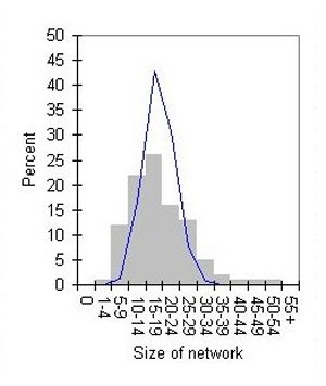
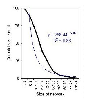
Compared to a Poisson distribution with the same mean (thin line) Cumulative, fitted to a power distribution (thin line)
Figure 1. Fischer's distribution of personal networks

1.5
Not all personal networks are fat-tailed, however. Bruggeman (2008: 34) pointed out that "the distribution of close friendships cannot have a fat-tail". As Aristotle (c300BC/1996: Book 9: x, 3) noted, "The number of one's friends must be limited" because, in modern terminology, the maintenance of social networks is not costless (Gilbert 2006). Such costs result in cut-offs in real networks (Watts & Strogatz 1998, Amaral et al 2000, Barthélemy et al 2003). Where those cut-offs fall depends on the type of network being modelled: the cut-off will be at a very small number if it is a model of 'confidants', with an average of two or three (Marsden 1987; McPherson et al 2001) but for acquaintances, the number could be in the hundreds or even thousands (Boissevain 1974: 108; Wetherell 1998). Thus any model should limit the size of personal networks because of the costs to individuals of maintaining them, while permitting the size of personal networks to vary (unlike, for example, Watts et al 2002) with the possibility, if required, of some individuals having much larger personal networks than average.

1.6
Furthermore, well-connected individuals tend to be connected to each other. Recently Newman (2003; Newman & Park 2003; Newman et al 2006: 555) suggested that a key feature of social networks that distinguishes them from other networks is the positive assortativity of the degree of connectivity i.e. those with many links link to others with many links. Bruggeman (2008: 35) has suggested that positive assortativity of degree is a type of homophily: sociable people like other sociable people. There does not appear to be agreement on how assortativity should be measured (see Newman 2003). Newman (2002; 2003) devised an index that equals one when there is perfect assortativity and lies between zero and minus one when there is complete disassortativity: a random network, for example, would produce an assortativity index of zero. Applying his measure to datasets of coauthorships, film actor collaborations, company directors and email address books, Newman (2002) found that his assortativity index was positive; while for technological networks (such as power grids and the internet) and biological networks (such as food webs and neural networks) the index was negative.

1.7
To sum up, we suggest that ideally a model of a large social network should have the following key characteristics : To this list, we would add that a general purpose social network model should not depend on strong assumptions that are likely to be applicable in only some social domains.

* Network models

2.1
Four basic types of network model recur in the literature: regular lattice, random, small-world and preferential attachment (also called scale-free). Examples of all four are shown in Figure 2. We now look at each in turn, comparing their characteristics to those of social networks as set out above.

Figure Figure
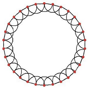
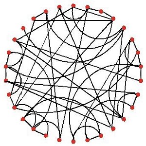
(a) Regular lattice: each node is linked to its four immediate neighbours (b) Random network: most nodes have three or four links.
Figure Figure
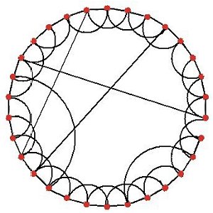
(c) Small world network: most nodes are linked only to their immediate neighbours. (d) Preferential attachment (scale-free) network: a few nodes have many links.
Figure 2. Examples of four basic models of networks: all with 30 nodes

2.2
The regular lattice, shown in the top left panel of Figure 2, represents the simplest type of network and is often used in cellular automata models. Its whole network density is low. The size of personal networks is limited and as many of one node's neighbours will also be neighbours of each other, there will be high clustering. But it fails to meet the other criteria and is therefore a poor model of a social network.

2.3
Models created by random linking have been analysed since the mid-twentieth century, starting with Erdos and Renyi (Newman et al 2006:12). An example is shown in the top right panel of Figure 2. However, as Barabàsi & Bonabeau (2003) pointed out:
despite the random placement of links…most nodes will have approximately the same number of links..Indeed, in a random network, the nodes follow a Poisson distribution with a bell shape and it is extremely rare to find nodes that have a significantly more or fewer links than the average.
Not surprisingly, the assortativity index of a random graph can be shown analytically to be zero (Newman 2002). Although such models display the short paths of social networks (Dorogovtsev & Mendes 2003: 105), it is hardly surprising that random networks fail to replicate other key features of social networks because we know that social networks are not in general created by making random links, although Aiello et al's (2001) recent analysis of phone call data suggested that, at the very large scale, random patterns may appear. So random networks are not good models of social networks either.

2.4
In 1998 Watts & Strogatz (1998) discovered that a few random re-wirings of a regular lattice produced a model with high clustering and short paths which they labeled a 'small-world', as shown in the bottom left panel of Figure 2. In effect, the small world model inherits its clustering from the regular lattice and its short paths from the random model (Dorogovtsev & Mendes 2003: 105). However, the small-world model does not produce nodes with high degrees of connectivity or display assortativity. Newman, Barabàsi and Watts (2006: 292)—and all three authors are named for emphasis—said that: "the small-world model is not in general expected to be a very good model of real networks, including social networks" and Crossley (2008) concurred.

2.5
Barabàsi & Albert (1999) proposed a scale-free network model created by preferential attachment, in which new nodes link to those that already have many links. This echoes what Merton (1968) termed the Matthew Effect—the rich get richer—and it has been argued that there is little new in Barabàsi's work (e.g. Scott 2009 forthcoming). Putting aside arguments about originality, the key point is that preferential attachment does not in general apply to social networks, the only exception found in the literature being sexual partners in Sweden (Liljeros et al 2001). People do not usually know who has many links and even if they did would not necessarily want to link to them, or the 'target' may not want to reciprocate. For instance, the failure of Milgram's and subsequent 'small world' experiments could be taken as evidence that people have only limited information about others' connections (Travers & Milgram 1969; Dodds et al 2003). As with the random network, the assortativity index of the preferential attachment model can be shown analytically to be zero (Newman 2002). This is hardly surprising given that the model generates a hub-and-spoke pattern as shown in the bottom right panel of Figure 2. While this model does produce a fat-tailed cumulative degree of connectivity, it is nevertheless also not a good model of social networks.

2.6
Table 1 summarises how the four basic network models score against the desirable characteristics of a social network model set out above. It shows that none of these standard network models seems to be very good models of real social networks.

Table 1: Summary of characteristics of the four basic network models

CharacteristicRegularRandomSmall-worldPreferential
attachment
Low density
Personal network size limited×
Variation in size of personal network×LimitedLimited
Fat-tail×××
Assortative××××
High clustering××
Communities×××
Short path lengths××

Agent-based social network models

2.7
In addition to these four basic models, a few others have been proposed recently in the agent-based modelling literature, for example, Pujol et al (2005) and Thiriot & Kant (2008). However, this paper takes a different approach and presents an agent-based social network model based on a minimum number of sociologically plausible assumptions and minimal data. The main inspiration has come from Watts et al (2002) in which "the probability of acquaintance between individuals" "decreases with decreasing similarity of the groups to which they belong". In their model, by tuning a single parameter, they could create a "completely homophilous world or isolated cliques" or at the other extreme "a uniform random graph in which the notion of individual similarity or dissimilarity has become irrelevant". Newman et al (2006: 292) suggested that this model is "possibly moderately realistic…based on a hierarchical division into groups". The idea of grouping is not new: for example, Pool & Kochen (1978) used "stratum".

2.8
The next section describes the basic structure of our model, which is extended in Section 4. Section 5 concludes. The models were implemented using NetLogo version 4.0.3 (Wilensky 1999) and can be found at http://www.hamill.co.uk/jasss08/.

* Basic Structure of the Model

3.1
The model is based on the ideas of social space and distance, which can be traced back to the early 1920s and was developed by (Heider 1958: 191) among others. McFarland and Brown (1973) suggested that social distance could be used in two distinct ways: to measure interaction, where those who are short distances apart are likely to interact (which they attributed to Bogardus), and to measure similarity where short distances imply similar characteristics (which they attributed to Sorokin (1927/1959: 3-10). For example, Wasserman & Faust (1994: 385-7) used social space to map similarity. More recently, Hoff et al (2002) used the concept of social distance on three 'classic' sets of network data to obtain better explanatory models than could be obtained using stochastic blockmodels. Finally, Edmonds (2006) argued that it is important to bring together physical and social spaces and the only way to do that is by using agent-based models. Models similar to that proposed below have been reported in the physics literature e.g. Barthélemy (2003) and Hermann et al (2003).

3.2
The setting for the model is what could be called a social map. While a geographical map shows how places are distributed and linked, the social map does the same for people. In this case, the closer any pair of agents, the stronger the tie between them. If it were considered that geographical distance alone determined social relationships, then this social map could become a geographical map with distance measured in miles or travel time. (For a discussion of social versus geographical distance, see McFarland and Brown 1973.)

3.3
The model is based on the concept of social circles, an idea dating back to at least Simmel (1902). The term circle was then used as metaphor. Yet a circle has a very useful property in this context: the formal definition of a circle is "the set of points equidistant from a given point", the centre (Weisstein 1998: 246). The circumference of a circle will contain all those points within a distance set by a radius and creates a cut-off, limiting the size of personal networks. For a given distribution of agents across the map, a small radius—which will henceforth be called the 'social reach' (sr)—can create a disconnected, gesellschaft-type society; a large social reach, a connected, gemeinschaft-type society. Alternatively, if the social reach is very small, it can be said to replicate a network of close family and friends: if larger, it becomes a model for larger networks of acquaintances.

3.4
Agents are only permitted to link with agents who can reciprocate; in other words, others whose reach includes ego. If A were to have a bigger reach than B then B could be in A's circle but not vice-versa, implying that A 'knows' B but B does not 'know' A, as illustrated in the left panel of Figure 3. Although there may be all sorts of asymmetries in the relationship between A and B and in their communication pattern, they must in some sense both 'know' each other. This definition thus excludes, for example, 'knowing' a celebrity seen on TV where there is no reciprocal contact. This assumption is discussed further in Section 5. The simplest way to achieve reciprocity is for all agents to have the same reach, as shown in right panel of Figure 3, but this is not essential, and will be relaxed later. However, we start by exploring the properties of the simplest model, in which all agents have the same social reach.

Figure Figure
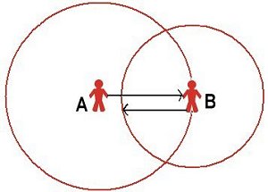
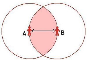
(a) No reciprocity: different social reaches: A knows B but B does not know A (b) Reciprocity with the same social reach
Figure 3. Reciprocity and social reach

3.5
Ceteris paribus, the size of personal networks will vary with the reach: the larger the reach, the larger the size of the personal network. To represent personal networks larger than 'intimates', a large total number of agents are required. The simulations presented in this paper use a population of 1,000 agents, meaning that there are almost half a million possible undirected links (1,000 × 999 / 2). These agents are randomly distributed across an unbounded grid of just under 100,000 cells, thus producing a population density of about one percent. (Further work could use more agents, different densities or distribute the agents differently, for example, using different densities in different parts of the space.) All reported results are based on the mean of 30 runs.

Degree and density

3.6
Hermann et al (2003) suggested that in such a spatial model, as the number of nodes increases and the social reach reduces, the connectivity distribution tends towards Poisson. Figure 4 shows how the connectivity of the agents changes as the social reach is increased: the distribution is flattened. For a social reach of up to about 30, the connectivity of nodes follows a Poisson distribution (the mean is the same as the variance) but for larger social reaches, the mean tends to exceed the variance.

Figure
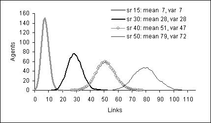
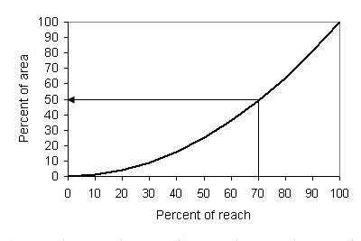
Figure 4. Degree of connectivity by social reach (sr)
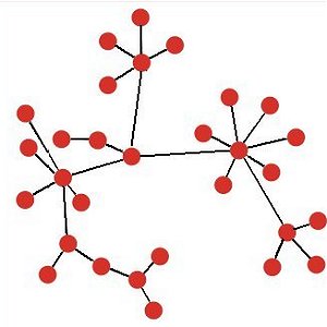
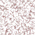
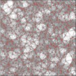
3.7
Although the personal networks of all the agents are defined by the same social reach, the numbers in each personal network will vary due to the randomness in the distribution of agents across the social map.

Figure Figure
Social reach = 15 Social reach = 30
Figure 5. Examples of how networks vary with the size of the social reach. (Red nodes, grey links.)

Clustering

3.8
Clustering is determined by the overlap of circles. If two agents are located very close to each other on the map, their circles will almost coincide and they will know most of the same agents. If there were complete overlap, the clustering coefficient would be one; if no overlap, zero. If, however, an individual is located on the circumference of another's circle, the overlap will cover 39 percent of the area of each circle. (This is shown in the top right hand panel of Box 2. For the mathematics, see the top left hand panel of Box 2.) Thus if agents are evenly distributed over the space, then the minimum clustering coefficient will be 0.39. Due to the geometrical properties of circles, and again assuming agents are evenly distributed, half the agents in a given personal network will be located outside 0.7 of the social reach (as shown in the middle panel of Box 2) and their clustering coefficient will be 0.56 or less (as shown in the bottom panel of Box 2).

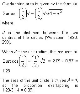
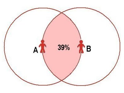
Box 2: Mathematics of circles

Figure

Figure
Figure
Figure

3.9
If the social reach is set very low, then there may be no agents in the overlapping area, giving a clustering of zero; alternatively, all the agents may be in the overlap area, producing a clustering coefficient of one. Thus, as illustrated in Figure 6, the clustering coefficient will vary more for smaller social reaches and as the social reach increases, the minimum of the clustering coefficient will tend to 0.39. (Box 3 explains how the clustering coefficient is calculated.)

Figure
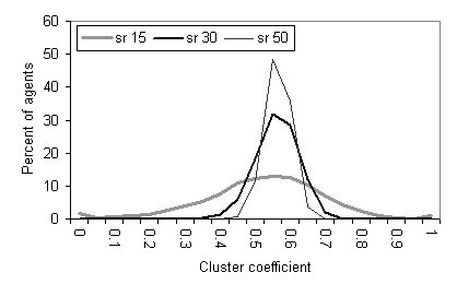
Figure 6. Cluster coefficient for the single-reach model with the social reach (sr) set at 15, 30 and 50


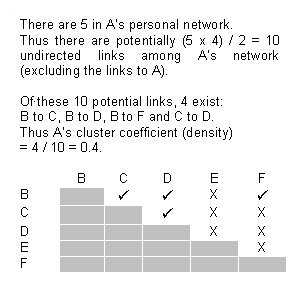
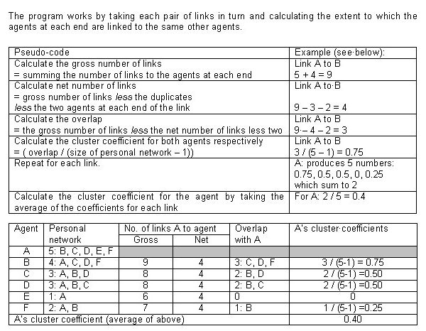
Box 3: Calculating the cluster coefficient: example and pseudo-code

FigureFigure
Figure

Path length

3.10
The minimum number of links from one agent to another, the path length, is determined by the size of the 'world', the social reach and the distribution of agents. Ignoring the distribution of agents, it is possible to calculate the theoretical path length. For example, a world of about 100,000 cells is created by a wrapping grid (torus) of 315 by 315 cells. An agent sitting at the centre of this grid will be at least 157 units from the edge (314/2). But the diagonal provides the furthest distance and by Pythagoras's theorem, this diagonal will be 222 units. The number of steps needed to cover this distance will depend on the social reach: the smaller reach, the more steps needed. For instance, if the social reach were set at 40, it would take a theoretical minimum of six steps to reach the farthest point, consistent with the famous six degrees (Travers & Milgram 1969, Watts 2004). But, this calculation is based on the maximum distance and most agents will therefore be closer, making the average path length shorter. Furthermore, no account has been taken of how agents are distributed across the map: optimal paths may not be attainable, and there is no guarantee that agents could find them.

Assortativity of degree

3.11
Intuition suggests that this model should produce assortative networks because those in densely populated regions will tend to have many links, as will those to whom they are linked (as Hermann et al 2003 suggested). This proves to be the case. The relationship between an agent's degree of connectivity and the average for those to which it is linked is positively correlated as indicated by the Pearson correlation coefficients (following Barthélemy 2003). For example, for a social reach of 30, the correlation coefficient averages 0.83 (sd 0.03). (Figure 7 shows a typical example.) For the lower reach of 15, it is 0.78 (sd 0.03) and for the higher reach of 50, 0.84 (sd 0.05).

Figure
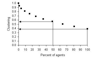
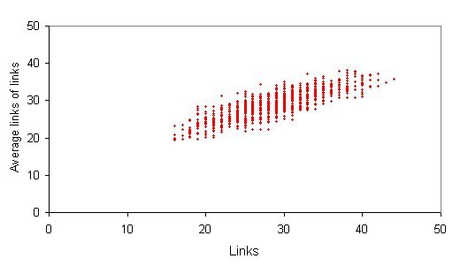
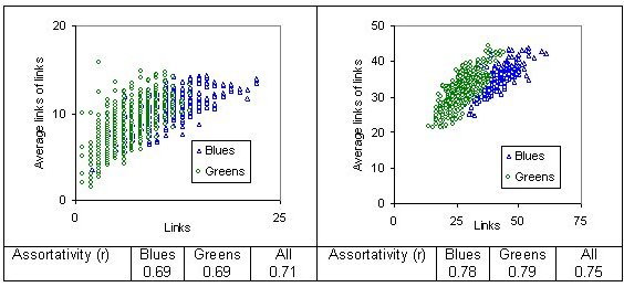
Figure 7. Assortativity of degree: typical example of correlation between degrees of connectivity: social reach of 30

* Extending the Model

Two reaches

4.1
The simple single-reach model is inflexible, the only parameters being population density and the size of the social reach, and while assortative it does not produce a fat-tailed distribution of connectivity. Also with larger social reaches all agents will have a clustering coefficient of at least 0.39. Yet Wellman's work suggested that the clustering coefficient averaged 33 percent among close associates, often kin, with a fifth having a density exceeding 50 percent (Scott 1991: 80-82).

4.2
These issues can be addressed by splitting the population in two and giving one group—call them Blues—a larger social reach than the other—call them Greens—but only permitting links between those who can reciprocate. Thus Green agents link only to other agents—Greens and Blues—within their small reach. But Blues with a large reach not only link to the Greens within their smaller reach but also Blues within the larger reach (see left panel of Figure 8). There are therefore two more parameters to adjust: the percentage of Blues with the larger social reach and the size of that reach. This has the effect of reducing the clustering coefficient for the Blues—for example, a Blue may share no Greens with a neighbouring Blue—and reducing path lengths for the Greens because a Blue in their personal network may provide a short cut to agents beyond their reach. In this way, a hierarchy is created. These features are illustrated in the right panel of Figure 8.

Figure Figure
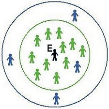
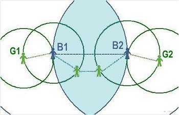
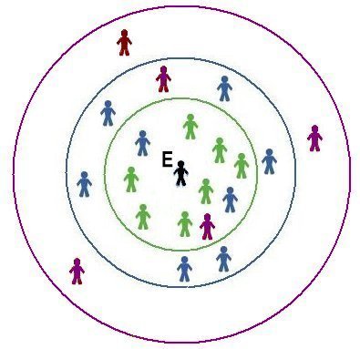
If E is a Green, then E links with everyone in the smaller (green) circle. If E is a Blue, then E also links to the three Blues within the larger (blue) circle A link between Blues B1 and B2 creates a short-cut and, for Blues, reduces clustering. The shaded area indicates overlap between the Blues' circles.
Figure 8. Two-reach model

4.3
The two-reach model in effect adds together two Poisson distributions, which can produce a distribution with larger variance and a fatter tail. Of course, if the percentage of Blues is small or if there is little difference between the two social reaches, the results from the two-reach model will tend towards that of the one-reach model. Figure 9 shows results for a pair of two-reach models with 25 percent Blues. In the first case (illustrated in the left column of Figure 9) the well-connected Blues have a social reach of 30 while that of the Greens is only 15; in the second case (illustrated in the right column), the Greens have a social reach of 30 while that of the Blues is 50.

4.4
Four results emerge:

Figure
Figure
Figure
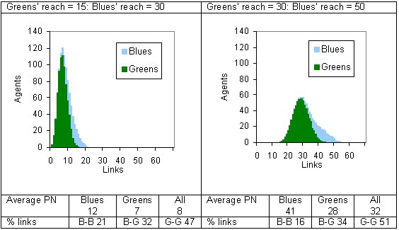
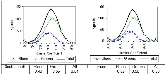
Figure 9. Examples of two-reach models: Blues 25 percent. (PN = personal network)

Three reaches

4.5
Adding a third reach increases the flexibility of the model still further. Figure 10 shows how this would work by adding Purple agents to the Greens and Blues. But as before, an agent can only link to those capable of reciprocating. If E is a Green, E would link to all 10 within the (smallest) green circle; if E were a Blue, E would also link to those in the (middle) blue circle giving a total personal network of 17; and if a Purple, to the Purples within the outer circle, giving a total of 20.

Figure
Figure 10. A three-reach model

4.6
To illustrate the flexibility of the three-reach model, we offer an example that demonstrates how two very different types of networks can be created by choosing different parameters. In both cases, the three social reaches are set at 30, 40 and 50 but in the 'elitist' case agents are distributed in the proportions 70/20/10 percent while in the 'democratic' case they are split evenly at 34/33/33 percent. The results are shown in Figure 11. The whole network density is 3 percent in the elitist case and 4 percent in the democratic case. In both cases the overall distribution of degrees of connectivity is wider than a Poisson distribution, notably so for the democratic case. But for each type of agent—Green, Blue or Purple—the distribution is approximately Poisson as indicated by the fact that the means are roughly the same as the variance. In other words, the Poisson distributions are added together to produce distributions ranging from a Poisson with a fat-tail to one that is starting to resemble a uniform distribution.

Figure
Figure
Figure 11. Two examples of degrees of connectivity in a three-reach model

4.7
Whether or not this flexibility is required and whether the additional complication is justified compared to the two-reach model will depend on the questions to be addressed by the modelling. For instance, the three-reach model would be appropriate if there were three distinct groups involved in the process being modeled, e.g. those who are globally connected, nationally connected or only regionally connected.

N-reaches

4.8
Each agent can have a different social reach provided that any pair of agents link only if both their social reaches permit. For example, if agent A has a social reach of 25 and agent B has a reach of 30, then providing the distance between A and B is no more than 25, they can link. Rather than choosing the percentage of agents with given social reaches as in the previous examples, it now becomes necessary to choose the distribution of the reaches and the parameters of those distributions. As noted in the Introduction, there is not an obvious choice.

4.9
Two types of distributions have been examined: uniform and Poisson. For the uniform distribution, minimum and maximum reaches were chosen and for the Poisson, just the mean (which then equals the variance). To illustrate this approach, Figure 12 compares the results from using Poisson and uniform distributions with using one or two reaches to produce an average personal network of around 30. Compared with using fixed reaches, using variable reaches reduces the assortativity and increases the range of size of both personal networks and the clustering coefficients, especially if a uniform distribution is used. However, neither the Poisson nor the uniform distributions of reach produce fat tails in this case, as shown in the bottom panel of Figure 12.

4.10
This approach is computationally more complex and increases the length of time taken for each run. Whether these costs outweigh the benefits is a matter of judgment and depends on the question being addressed.

Figure
Figure
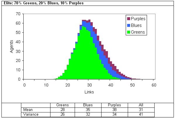
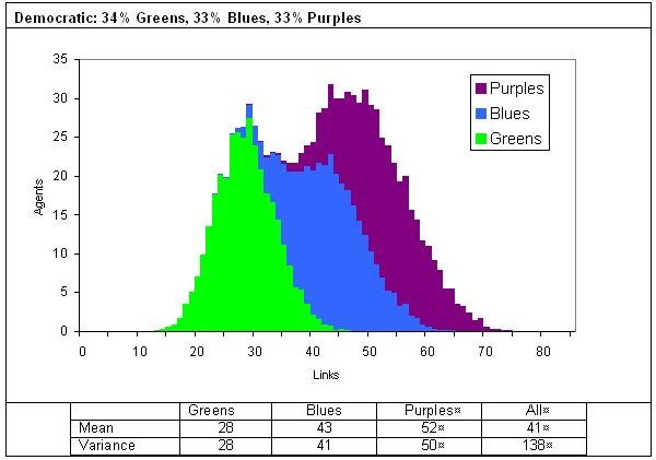
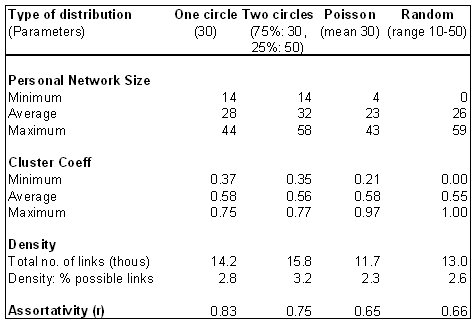
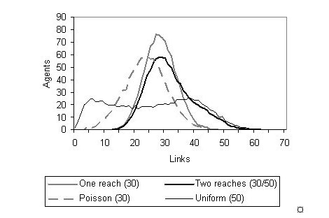
Figure 12. Comparison of various ways of producing an average personal network of around 30

* Discussion and conclusion

Properties of the model

5.1
We have presented a simple structure to create large social networks in agent-based models that, to some extent, meet all the criteria set out in the Introduction in that it creates networks that:

Sociological assumptions

5.2
The final criterion was that the model should not rest on strong sociological domain specific assumptions. Like any model, it is a simplification of the real world. There are two key assumptions underlying the model, which we consider to be sociologically acceptable at least for relatively abstract modelling: symmetrical relationships and the use of two dimensional space.

5.3
The model assumes that personal networks can be added together to create a social network. This requires that relationships be symmetrical. Whether this is realistic depends on what aspect of social relationships are being analysed. For example, within a kinship group, the biological relationship must be symmetrical: if A is a cousin of B, then B is, by definition, a cousin of A. But this may not hold for other types of social networks. It is well-established that many relationships are asymmetrical in strength (Wellman 1988: 40-41): A loves B but B only likes A. Such asymmetrical social relationships can be modeled using directed links (i.e. distinguishing between links to a node and links from a node (Wasserman & Faust 1994: 121, 126)) and weighted links to reflect the 'traffic', somehow defined, that passes along them. This is something to be explored in further work: in the meantime, this model can be used if some sort of averaging is assumed.

5.4
The second key assumption is the use of two dimensions for the social map. This imposes limits on the structure of the network by what can be called the parallelogram problem. Consider four agents A, B, C and D. If A, B and C are linked and A, B and D are also linked, then the distance between C and D is fixed by the laws of geometry as illustrated in Figure 13. However, if C and D both know a fifth agent, E, who does not know A and B, it may not be possible to show both links on a two dimensional map although using three dimensions it would be. But to provide insights, models must be simple. This model is intended to reproduce certain key features of social networks, and to do that simplifications have to be accepted.

Figure
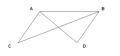
Figure 13. The parallelogram problem

Conclusion

5.5
We have presented a simple structure to produce large social networks in an agent-based model that represents social networks better than the standard network models: regular lattice, random, small-world and preferential attachment. It is based on the metaphor of social circles and makes use of the geometrical properties of circles. The radius of the circle has been labeled the social reach. The two-reach model seems to be particularly useful in that, although simple, it provides the essential features of a social network. However, three or more reaches can be used, and even different reaches for each agent, but whether the costs in terms of more complicated programs and longer run-times are justified will depend on the question being addressed.

5.6
There is much scope for further work including increasing the number of agents, distributing agents differently, changing the distributions of connectivity, incorporating strength of ties, adding dynamics and increasing interactivity between agents.

* Acknowledgements

This work was supported by Microsoft Research through its European PhD Scholarship Programme. The authors are also grateful to participants in ESSA '08, the JASSS reviewers and members of CRESS for their helpful suggestions.

* References

AIELLO, W., Chung F. & Lu, L. (2000/2006) A random graph for massive graphs. In Newman, M., Barabasi, A-L. & Watts, D.J. (2006) The Structure and Dynamics of Networks. Princeton University Press.

AMARAL, L. A. N., Scala, A. Barthélemy M., & Stanley H. E. (2000) Classes of small-world networks. PNAS. Vol. 97. No. 21 pp.11149-11152.

ARISTOTLE (c300BC/1996) The Nicomachean Ethics. Ware. Wordsworth.

BARABSI A-L. & Albert, R. (1999) Emergence of Scaling in Random Networks. Science, New Series, Vol. 286, No. 5439., pp. 509-512.

BARABSI A-L, & Bonabeau, E. (2003) Scale-Free Networks. Scientific American (May) pp.52-59.

BARTHÉLEMY, M. (2003) Crossover from scale-free to spatial networks. Europhysics Letters. 63 pp.915-912.

BOISSEVAIN, J. (1974/78) Friends of Friends: Networks, Manipulators & Coalitions. Oxford. Basil Blackwell.

BRUGGEMAN, J. (2008) Social Networks. London. Routledge.

CALDERELLI, G. (2007) Scale-Free Networks: Complex Webs in Natural, Technological and Social Sciences. Oxford. Oxford University Press.

COULTHARD, M., Walker, A. & Morgan, A. (2002). People's perceptions of their neighbourhood and community involvement: Results from the social capital module of the General Household Survey 2000. London. National Statistics. The Stationery Office.

CROSSLEY, N. (2008) Small-world networks, complex systems and sociology. Sociology. Vol 42, No. 2, pp.261-277.

DODDS, P.S., Muhammad, R. & Watts, D.J. (2003) An Experimental Study of Search in Global Social Networks. Science, 8 August pp. 827-829.

DOROGOVTSEV, S. & Mendes, J. (2003) Evolution of Networks: From biological nets to the Internet and WWW. OUP.

EDMONDS, B. (2006) How are physical and social spaces related? In Billari, F.C., Fent, T.; Prskawetz, A. & Scheffran, J. (eds.) Agent-Based Computational Modelling Springer. (Downloaded on 10 March 08 from cfpm.org/cpmrep127.html).

FISCHER, C.S. (1982) To Dwell Among Friends. Chicago. University of Chicago Press.

GILBERT, N. (2006) Putting the Social into Social Simulation. Keynote address to the First World Social Simulation Conference, Kyoto.

HEIDER, F. (1958) The Psychology of Interpersonal Relations. New York. Wiley.

HERMANN, C. Bathélemy, M. & Provero, P. (2003) Connectivity distribution of spatial networks. Physical Review E 68 026128.

HOFF, P. D., Raftery, A. E. & Handcock M. S. (2002) Latent Space Approaches to Social Network Analysis . Journal of the American Statistical Association, Vol 97, No 460, 1090-1098

LILJEROS, F., Edling, C., Amaral, L., Stanley, H.E., & Aberg, Y. (2001/2006) The web of human sexual contacts. Nature. Vol 411, 21 June. 907-8.

MARSDEN, P.V. (1987) Core discussion networks of Americans. American Sociological Review. Vol 52. No.1. pp.122-131.

MCFARLAND, D.D. & Brown, D.J. (1973) Social Distance as a Metric: A systematic Introduction to Smallest Space Analysis. In Laumann, E.O. Bonds of Pluralism: The Form and Substance of Urban Social Networks. New York. Wiley.

MCPHERSON, M., Smith-Lovin, L. & Cook, J.M (2001) Birds of a Feather: Homophily in Social Networks. Annual Review of Sociology. 27. pp.415-444.

MERTON, R.K. (1968) The Matthew Effect in Science. Science, New Series, Vol. 159, No. 3810 (Jan. 5, 1968), pp. 56-63.

NEWMAN, M. (2002) Assortative mixing in networks. Physical Review Letters. Vol 89. No.20. 208701.

NEWMAN, M. (2003) Mixing patterns in networks. Physical Review E. 026126.

NEWMAN, M., Barabasi, A-L. & Watts, D.J. (2006) The Structure and Dynamics of Networks. Princeton University Press.

NEWMAN, M. & Park, J. (2003) Why social networks are different from other types of networks. Physical Review E. Vol 68, 036122

POOL, I.S. & Kochen, M. (1978) Contacts and Influence. Social Networks. 1. pp.5-51.

PUJOL, J. M., Flache, A., Delgado, J. & Sanguesa, R. (2005) How Can Social Networks Ever Become Complex? Modelling the Emergence of Complex Networks from Local Social Exchanges. Journal of Artificial Societies and Social Simulation 8(4)12 https://www.jasss.org/8/4/12.html.

SCOTT, J. (1991) Social Network Analysis: A Handbook. London. Sage.

SCOTT, J. (2009 forthcoming) Handbook of Social Networks.

SIMMEL, G. (1902) The Number of Members as Determining the Sociological Form of the Group.I. American Journal of Sociology. Vol 8, No.1. pp1-46.

SOROKIN, P.M (1927/1959) Social and Cultural Mobility. London. Collier-Macmillan.

THIRIOT , S. & Kant, J-D. (2008) Generate country-scale networks of interaction from scattered statistics. Presented at ESSA 08, Brescia, Italy.

TRAVERS, J. & Milgram, S. (1969) An Experimental Study of the Small World Problem. Sociometry. Vol (32) 4. pp 425-443.

WASSERMAN, S. & Faust, K. (1994) Social Network Analysis. Cambridge University Press.

WATTS, D.J. (2004) Six Degrees: The Science of a Connected Age. London. Vintage. Watts, D.J., Dodds, P.S., & Newman, M. (2002) Identity and search in social networks. Science. Vol 296. 17 May.pp.1302-1305

WATTS, D.J. Dodds, P.S., & Newman, M. (2002) Identity and search in social networks. Science. Vol 296. 17 May. pp 1302-1305.

WATTS, D. J. &. Strogatz, S. H. (1998) Collective dynamics of 'small-world' networks. Nature. Vol 393 4 June.

WEISSTEIN, E. (1998) CRC Concise Encyclopedia of Mathematics. Boca Raton. CRC Press.

WELLMAN, B. (1988) Structural analysis: from method and metaphor to theory and substance. In Wellman, B. & Berkowitz, S.D. (eds) Social Structures: A Network Approach. Cambridge. Cambridge University Press. Pp 19-61.

WETHERELL, C. (1998) Historical Social Network Analysis. International Review of Social History. Vol. 43. Supplmement 125-144

WILENSKY, U. (1999) NetLogo. http://ccl.northwestern.edu/netlogo/. Center for Connected Learning and Computer-Based Modeling, Northwestern University, Evanston, IL.

WONG, L.H., Pattison, P. & Robins. G. (2006) A spatial model for social networks. Physica A. 360, pp. 99-120.

----

ButtonReturn to Contents of this issue

© Copyright Journal of Artificial Societies and Social Simulation, [2009]