©Copyright JASSS

JASSS logo ----

Pedro Ribeiro de Andrade, Antonio Miguel Vieira Monteiro, Gilberto Câmara and Sandra Sandri (2009)

Games on Cellular Spaces: How Mobility Affects Equilibrium

Journal of Artificial Societies and Social Simulation vol. 12, no. 1 5
<https://www.jasss.org/12/1/5.html>

For information about citing this article, click here

Received: 01-Apr-2008    Accepted: 04-Jan-2009    Published: 31-Jan-2009

PDF version


* Abstract

In this work we propose a new model for spatial games. We present a definition of mobility in terms of the satisfaction an agent has with its spatial location. Agents compete for space through a non-cooperative game by using mixed strategies. We are particularly interested in studyig the relation between Nash equilibrium and the winner strategy of a given model with mobility, and how the mobility can affect the results. The experiments show that mobility is an important variable concerning spatial games. When we change parameters that affect mobility, it may lead to the success of strategies away from Nash equilibrium.

Keywords:
Spatial Games, Agent-Based Modelling, Mobility, Satisfaction, Chicken Game, Nash Equilibrium

* Introduction

1.1
Over the last years, the role of spatial self-structuring in the study of games has drawn a lot of attention. Particularly, games with spatially explicit factors have proven to be useful for modelling biological and economic environments (Nowak and Sigmund 2000). The purpose of such games is to assess the effects that spatial structures have on adaptation strategies of agents, mainly in the study of the evolution of altruistic behaviour. Adding a spatial component to the models (usually in the form of grids) often displays different features from models with well-mixed populations. For example, the evolution of interspecific mutualism cannot be explained by an unstructured population through the iterated continuous Prisoner's Dilemma (Scheuring 2005).

1.2
Most of the games on grids use a straightforward extension of non-spatial games, with each cell containing a single agent that interacts with its neighbourhood. If the agents interact only with fixed neighbours, there will be no need to recognize and remember the opponents (Nowak et al. 1995). This arrangement allows the same game to be repeated, and the results influence how the agents populate the cellular space. As an example, Nowak and May study the spatial Prisoner's Dilemma, in which a cell is given to the strategy with highest payoff in the neighbourhood, if it is greater than the current payoff (Nowak and May 1992).

1.3
A spatial arrangement may lead to different results because it changes the way with which agents interact, from well-mixed confronts to local competitions. But there is a second characteristic of space that may affect the development of spatial models: the mobility. Agents can move in the space, changing their spatial locations and making the local relations dynamical.

1.4
The literature of spatial models presents two definitions of mobility. First, analytical models using replicator-diffusion equations often call mobility the spread of a strategy in the space (Ferrière and Michod 2000). The second definition works with the mobility of an individual agent, which can move to an empty neighbour cell. Examples of such models can be found in studies of cooperation (le Galliard 2003 et al.; Epstein 1997), linguistics (Kosmidis et al. 2005), and evolution of cancer (Mansury et al. 2006).

1.5
In all works that involve numerical simulation, the mobility of an agent is an automated action, which always depends on a social opportunity as, for instance, an old neighbour has left an empty cell. Moreover, that happens even if the current spatial location is favourable to the agent. However, instead of moving to the neighbour cell as soon as possible, a "rational" agent would ask: why should I move if I am getting good results? That is a common strategy adopted in spatial models which do not use games, such as in Zhang (2004) and Beltran et al. (2006). In these works, the agent compares the current satisfaction with the satisfaction in the new spatial location, moving when its satisfaction increases with the change.

1.6
In this work, we explore the question of mobility within the context of non-cooperative games, more precisely using the chicken game. We propose a new spatial model by defining mobility in terms of the satisfaction of an agent with its current spatial location. Agents use mixed strategies to compete, and decide to move according to their payoffs. An agent does not depend on a social opportunity for leaving its spatial location: it can move to a new spatial location even if it is already populated with other agents. Agents have complete freedom to move; there is no cost or constraint to do so. In this framework, instead of competing with their neighbours, the agents compete with each other within the same cell.

1.7
Contrary to what happens in the literature of spatial games, in this work we have a clear separation between the concepts of cell and agent. There are many real world situations where it is useful to consider agents moving from one cell to another. Such cases are common in geographical space, where a cell is usually a container that has properties which might be different from its neighbours. Take the case of land use change models. Land use change cells differ not only in their locations, but also in properties such as topography, water availability, and temperature. In these and similar cases, a cell can contain a small community of agents. Agents interact with their community (inside the cell) and if dissatisfied, they will try to find a more friendly community elsewhere in space. Combining interaction within cells and movement between cells allows new insights when modelling games in space.

1.8
We are particularly interested to study the relation between the Nash equilibrium and the winner strategy of a given spatial model with mobility, and how the definition of mobility can affect the results. In a nutshell, we try to answer the following questions: is Nash equilibrium the best strategy in a competition for space where the agents can move according to the results of the games? If not, in which cases, and how can it help to define the best strategy? Also, how does the proposed definition of mobility possibly affect the results?

* Related Works

Non-cooperative Games and Nash Equilibrium

2.1
A non-cooperative game is an n-person game where the actions of each player are independent, without any collaboration or communication with the other players. In an n-person game we have, for each player:
  1. a finite set of pure strategies (actions);
  2. a payoff function, that maps all n-tuples with the individual pure strategies to real numbers.

2.2
One mixed strategy is a collection of non-negative numbers adding up to 1, corresponding to probabilities of using each of the pure strategies. The mixed strategy defines the tendencies of a player. Each time it plays, it will choose randomly one of its pure strategies, based on the probabilities defined by the mixed strategy.

2.3
For example, let us take the chicken game. Two players have the choice to escalate ( E) or not to escalate ( ∼E) a brawl. If none of them escalates, nothing happens. If only one escalates, the other player runs away, and the winner receives 1 from the coward player. But, if both decide to escalate, each player pays 10 due to medical care. This game is said to be symmetric, because both players employ the same pure strategies and payoffs, as shown in Table 1. Given that this game has only two pure strategies, we denote by sx, 0 ≤ x ≤ 1, the mixed strategy of escalating with probability x.

Table 1: Game payoffs, in pairs (A, B)

B escalatesB does not escalate
A escalates(-10, -10)(+1, -1)
A does not escalate(-1, +1)(0, 0)

2.4
Nash proved that, given any non-cooperative game of n players, there is always an equilibrium point. This point is a set of mixed strategies for each player that, if a player individually changes its mixed strategy, the best result it may get will be the same as in the equilibrium (Nash 1951). No player has incentive to deviate one-sidedly from its strategy as long as the other players remain in the equilibrium. This is known as the Nash equilibrium.

2.5
For example, let A and B be two players of the chicken game, with strategies sa and sb, respectively. The expected payoff of player A is -10sasb + sa - sb. If A knew exactly the value of sb, it would be possible to calculate the best action for it. If sb is greater than 10%, the best choice for A is never to shoot (sa = 0), implying in a payoff of -sb. If sb is less than 10%, A should always shoot (sa = 1), because its payoff would be 1-11sb. But, if sb is exactly 10%, all strategies for A lead to the same payoff (-0.1). Therefore, if sa is also fixed at 10%, no other strategy could augment its payoff against A by changing its own mixed strategy. Applying the same reasoning for B, we arrive to the conclusion that when both players follow s0.1 the game is at Nash equilibrium.

2.6
But this idea of equilibrium may cause controversy in some games. Most game theorists agree on s0.1 as the rational solution for this game, but the argument is somewhat tenuous (Sigmund 1993). In the chicken game, although deviating from the equilibrium does not increase the utility of the player, it does not decrease as well, as long as the other player stays in the equilibrium. Therefore, it is not a strict equilibrium.

2.7
A clear explanation can be found when it is played not only by two players, but within a population. Maynard Smith viewed this game in a population-dynamical setting (Maynard Smith 1982). In his model, a large number of players meet randomly in contests where they have to decide whether to escalate or not. If the estimated overall probability is greater than 0.1, it is better not to escalate. If it is less than 0.1, it is better to escalate. But if it is exactly 0.1, then there is no better strategy than s0.1. In this sense, self-regulation leads to s0.1 - self-regulation not between two players, but within a population. Nash has also proposed a similar interpretation for the equilibrium points, the mass-action (Nash 1950), which was forgotten for decades in his unpublished thesis. In this work, we will study how this non-strict equilibrium behaves in a spatial context with the agents' mobility based on the results of the games.

Spatial Games

2.8
Recently, new models with different neighbourhood topologies have been proposed to study games in the space. The proposals include variations of grids, graphs, and some in between structures (Biely et al.2007; Cassar 2007; Duran and Mulet 2005; Soares and Martinez 2006; Vainstein and Arenzon 2001; Vukov and Szabò 2005; Wu et al. 2006). Ohtsuki and Nowak (2006) have shown that, in the limit of weak selection, models with different topologies can be described only by changing the payoff matrix . Although these models have different topologies, agents have the same characteristics: they are fixed in the space, have only a pure strategy, play with neighbours, and may spread their strategies to the neighbourhood according to the result of the games.

2.9
Commonly, the result of the game is only used for defining a new spatial arrangement, but it by itself does not have a future effect in the model. Feldman and Nagel (1993) propose a model where cells are not updated by a new strategy at the end of the turn. Instead, each cell must pay a fee each turn to stay in the model, and a neighbour strategy will replace it only if its savings end. Epstein (1997) studies the evolution of cooperation in a model where agents may be removed from the model if they reach zero or less wealth, since the payoff matrix has negative entries.

2.10
Beltran and others (2006) propose a model where agents move in a lattice trying to minimize their dissatisfaction. The satisfaction is a function of the difference between the real distances it keeps from the other agents and the ideal distances it wants to keep from them. Zhang (2004) studies a segregation model, where agents may exchange their spatial locations according to a definition of satisfiability. In both models, only one agent can be within a cell in each time step.

* The proposed model

3.1
The model takes place in a cellular space. A cellular space is an environment with cells connected by neighbourhood relations. The simplest example of a cellular space is a grid, with square cells having four touching neighbours. The objective of using the term cellular space instead of graph is to distinguish the meaning of a neighbourhood: instead of connecting individuals, as in typical spatial games, a cellular space simply connects cells, defining a spatial proximity relation.

3.2
The cellular space is always populated with individuals called agents. Each agent belongs to a single cell, which has enough space for it to live. Initially, each cell contains a set of agents, which have to compete for the space through a non-cooperative game. Whenever an agent is playing a non-cooperative game, we call it a player, but one agent has other characteristics besides those of players in the sense of a non-cooperative game (pure and mixed strategies), as it will be seen below.

3.3
The basic assumption of our model is that when an agent arrives at a cell (as well as in the beginning of the model), it is satisfied with its cell, and thus no agent will move unless it is dissatisfied. Two agents within the same cell may play a non-cooperative game competing for it, and the result of each game affects directly their individual satisfaction with the current cell. This is the only memory an agent has, and it is called local satisfaction. The local satisfaction starts with a positive value when an agent arrives at a cell. Whenever it reaches zero or less, the agent randomly picks a neighbour cell and moves to it, looking for a better cell to compete for. Given that, the movement of agents in a cellular space can be characterized as a random walk.

3.4
Each agent also has a global satisfaction, starting with a positive value significantly greater than the local satisfaction. As the local satisfaction, it is affected by the payoffs of the games. All agents have the same global satisfaction at the beginning of the model. An agent that got dissatisfied many times and its global satisfaction reaches zero or less leaves the model. In the models we propose in this work, the global satisfaction does not affect the agents's behaviour.

3.5
To create a metric for measuring satisfaction, we say the satisfaction of an agent is measured by its capital. Local satisfaction represents the limit of capital one can dispend for a cell. Global satisfaction corresponds to the initial capital assigned to an agent, thus it leaves the model when its money ends.

3.6
Agents differ in one characteristic: the mixed strategy. We divide the agents in groups of equal size. Two agents within a group share the mixed strategy, but they cannot communicate nor identify each other. Although the agents compete individually, they represent a strategy that is going to be studied in a spatial context. To represent the fittest agents along the model execution, the agent with higher global satisfaction in a cell will be its owner, because, at least at first sight, it has more chance of surviving than any other in that cell. If two agents have the same amount of money in a given cell, the agent that stands there for a longer time is its owner. In the first turn of the model, we divide the owners equally among each group.

3.7
The model has a finite number of turns, each one with two steps. The first step sets up and carries out the games. Supposing the game has two players, we randomly choose pairs of agents in each cell, and then carry out the game with each pair. Cells with an odd number of agents have one random idle agent, and no agent will play more than once in each turn. The same logic can be applied to games with more than two players.

3.8
The second step defines the dynamical part of the model. Once each agent already knows its payoff, it updates its local and global satisfactions with the payoff. Then, it checks if any satisfaction has reached zero or less to perform a movement or leave the model. The model runs until it reaches a stable state, which happens when there is at most one agent in each cell, or when their satisfaction stops to decrease. Whenever the model arrives at one of these situations, we say that it is at equilibrium.

3.9
There are two differences between the general model proposed here and the ones proposed in the literature. First, and most importantly, the model separates agents from space. The agents compete for space but they are not equivalent to the space itself. Neighbourhood relations point to where an agent can go, trying to find a better cell to fight for. Second, an agent plays with a random opponent inside the same cell and, as agents can move, the chance of two agents meet more than once can be very small. Given that, we only allow mixed strategies, and no meta-strategies such as Tit-For-Tat (Axelrod 1980) or Pavlov (Nowak and Sigmund 1993), because this model is not a repeated game.

3.10
A model of games on cellular space can be formalized as a 9-tuple: M = ( C, n, S, p, A, s, k, g, l), where Therefore, given sx, we have s ( sx, E) = x and s ( sx,∼E) = 1 - x. An agent using a mixed strategy commits to a randomization device. Each time the agent plays, it chooses a pure strategy based on the probabilities specified by the mixed strategy.

3.11
As an example of model, the following denotes the traditional chicken game: Mc = ( Cc, 2, { E, ∼E }, u, { sa, sb }, s, 1, ∞, ∞). The cellular space Cc has a single cell containing two agents, each one coming from a different group, one from sa and the other from sb. They have the same set of possible actions, "escalate" and "not escalate," and the same payoff matrix u (shown in Table 1), but they do not have to follow the same mixed strategy. Both agents always stay in the only cell and never leave the model.

3.12
In this work, we are particularly interested in applying the chicken game within this general model. The expected payoff of this game is almost always negative, only in the case where both players never escalate the expected payoff is 0. Therefore this game fits in with the requirement of reducing their satisfaction to make them move. C is always a squared grid with 20 x 20 cells, such that the possible movements of an individual are at most to four neighbours (up, down, left and right). Cells on the edges have only three alternatives for movement, and cells on the corner have only two.

* A first experiment

4.1
As first experiment, we divide the agents equally in the following three groups:
  1. Always use the pure strategy seemingly more profitable, escalate, because it is the only way to earn something, and the opponent will have a payoff at most as bad as its;
  2. Choose randomly a pure strategy in each game (escalate with chance of 50%);
  3. Follow Nash equilibrium, escalating with chance equal to 10%.

4.2
Initially, there are three agents of each strategy competing in each cell, summing-up nine agents by cell. Each agent starts the model with $200 and, inferring that loosing $10 twice without earning any money is enough to turn an agent dissatisfied, we chose $20 to be the local satisfaction. Therefore we have M 0 = (C, 2, { E, ∼E }, u, { s0.1, s0.5, s1.0}, s, 1200, 200, 20), where s 0.1 follows Nash equilibrium, s 0.5 plays by using a coin toss, and s 1.0 always escalates.

4.3
This model is stochastic, and we are interested in the convergence more than in showing numerical results. Clearly, M 0 always converges to the state where there is at most one agent in each cell, but when we say convergence, we aim at verifying whether the results obtained by each strategy in the simulations are similar.

4.4
We run the model 50 times to verify convergence and, although there are three stochastic components in the model (movement, escalating, and confronts), the simulation results have a low standard deviation. Also because of randomness, the simulations have different number of turns until they end.

4.5
Figure 1 shows the results of one realization, and Figure 2 shows the spatial distribution of the owners along a simulation. Clearly, the number of agents and the total amount of money of each group decrease along the simulation, and the more ambitious a strategy is, the sharper is the fall of the money and the number of agents following that strategy. Figure 1(c) also shows the mean value and the standard deviation of the experiments, plotted as arrows on the right side. There are some empty cells at the end of the simulation, which happens because, when there are only two agents in a cell, both might escalate, lose $10, reach the threshold, and decide to leave the cell.

Figure
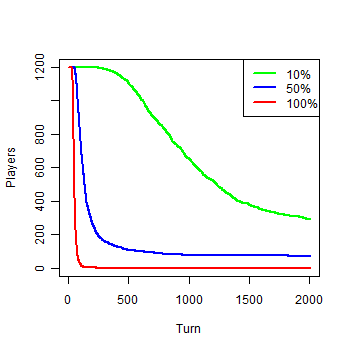
Figure 1a. Results of the first experiment: a) Number of agents

Figure
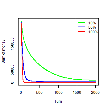
Figure 1b. Results of the first experiment: b) Money by groups

Figure
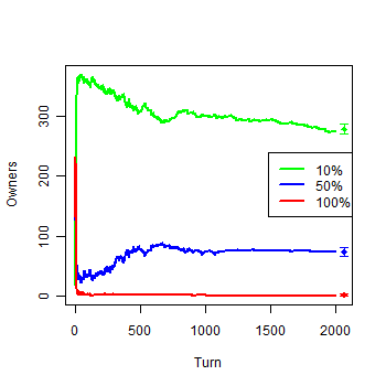
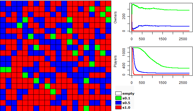
Figure 1c. Results of the first experiment: c) Owners by groups

Figure
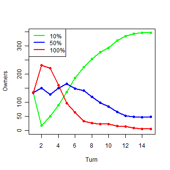
Figure 1d. Results of the first experiment: d) Owners in the first 15 turns

Figure
Figure 2. Example of a run of the first experiment

4.6
The results show that the group following equilibrium has achieved most of the cells, despite the early misfortune shown in Figure 1(d). There are, nevertheless, some agents of other strategies at the end of the model. Equilibrium agents got the best results at the end, but they did not reached the majority by their own victories, it was indeed because the other strategies have lost their money faster. It is possible to see clearly that more aggressive agents destroy themselves rapidly and, therefore, following equilibrium yields a better chance of surviving. But, when there are a few aggressive agents in the model, they can avoid themselves and conquer some cells, justifying the growing number of cells conquered by s 0.5 at the end of the simulation. As the non-equilibrium strategies lose money faster than equilibrium ones, the initial money has a clear impact on the model, and agents following the equilibrium get more advantage of its increase. Simulations with higher values of initial money have shown that the difference between the number of cells of s 0.1 and s 0.5 becomes even larger.

4.7
Figure 3 shows the number of agents of each strategy that move during the first 150 turns of the model. More aggressive agents reach the threshold more frequently, until they start to leave the model. After the 30 th turn, the number of movements decreases until the model stabilizes.

Figure
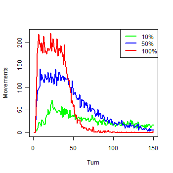
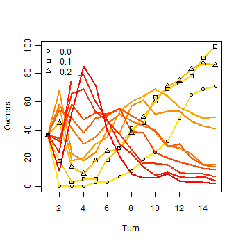
Figure 3. Movements of each group in the first 150 turns

* Model variations

5.1
In M 0, Nash equilibrium is the best strategy for the competition against the other two chosen strategies. This section describes three other experiments, in order to verify whether the equilibrium strategy fares better also in other arrangements. In the first variation, we assign an infinite amount of money to each agent. In the second one, an extra amount of money is assigned to both agents after they play a game. We analyse how the model behaves when money is less constrained in both experiments. In the last experiment, we use eleven strategies instead of only three.

Infinite amount of money

5.2
The initial amount of money can be large enough to keep all the agents alive until the end of the simulation. With it, the model will never converge to a stable state, because the agents will move indefinitely. We have the following model: Minf = (C, 2, { E, ∼E }, u, { s 0.1, s 0.5, s 1.0}, s, 1200, ∞, 20). As we can see in Figure 4(a), this model has a continuous repetition of the instability previously shown in the first 30 steps of Figure 3. This instability is favourable to s 0.1, which owns more than 85% of the cells, from the 30 th turn until the end of the simulation, as we can see in Figure 4(b). The Figure also shows the mean and standard deviation of each strategy.

Figure
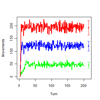
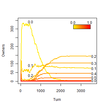
Figure 4a. Model with infinite Money: a) Movements of each group

Figure
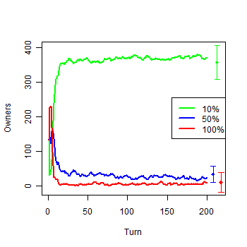
Figure 4b. Model with infinite Money: b) Owners by groups

5.3
Supposing a non-spatial environment, with agents meeting each other with equal probability, we can calculate the expected payoff of each strategy, deduce the number of movements, and compare it with the mean number of movements of the simulation. The expected payoff of an agent is the mean expected payoff against each group. The number of turns necessary for an agent of a given group to reach the threshold for moving is straight from this value, since the local satisfaction is $20. Then, as there are 1200 agents of each group, the mean number of agents that would move each turn can be calculated. Table 2 shows these values, and in the lower part there is the difference between the expected movements in a non-spatial model and the mean value of the movements in the experiments with infinite money. Clearly this value is less than in a non-spatial environment because each cell with an odd number of agents has one idle agent. Agents in space also reduce the expectations of a non-spatial environment because an agent that leaves a cell may find itself in a new one that happens to be more convenient. But this reduction is not equal for each strategy: the more an agent escalates, it can realize an unfavourable arrangement earlier, leaving the cell faster than the other strategies. It justifies why the decrease is proportional to the probability of escalating.

Table 2: Impact of the escalating probability in the movement

s0.1s0.5s1.0
Against s0.1-0.10-0.10-0.10
Against s0.5-0.90-2.50-4.50
Against s1.0-1.90-5.50-10.00
Mean-0.97-2.70-4.87
Turns before an agent moves20.617.404.10
Expected movements by turn58.22162.16292.68
Movements with infinite money47.25123.20196.13
Difference10.9738.9696.55
Decrease (%)18.8424.0232.98

Extra gain

5.4
The second variation still concerns the reduction of the number of agents along the model. But instead of increasing the initial amount of money, as in Minf, we give an extra gain of capital to both agents at the end of each game, with the objective of keeping them alive. We describe a model with extra gain k as: M gk = (C, 2, { E, ∼E }, u + k, { s 0.1, s 0.5, s 1.0}, s, 1200, 200, 20). As we increase all the payoffs by a constant value, the expected payoff of each agent also increases with this value, and thus the equilibrium point does not change (Nash 1950). We explore six models with different values of extra gain to verify how it affects the results. They are: M g +0.1, M g +0.2, M g +0.4, M g +0.8, M g +1.6, and M g +3.2.

5.5
Figure 5 shows the number of agents in the six models at the end of the 3000th turn. After that, the models have only some minor changes. The total number of agents that survive rises with the extra gain, but agents with a higher escalating probability have a lower tax of increase. Note that, contrary to the variation of infinite money, some agents are still being removed from the model, as they reach the global threshold.

Figure
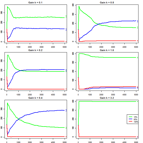
Figure 5. Agents of each group in the model with extra gain after turn 3000

5.6
As the extra gain increases, agents that escalate less often stop reaching the threshold for moving and start to stand still, because they gain more money than lose. Figure 6 shows the owners in the six models. The first strategy to lose mobility is s 0.1. Because of it, from gain M g +0.2 until M g +0.8, it loses the majority to s 0.5. After the gain +0.4, s 0.5 also starts to lose mobility, then cells, and finally in the model M g +1.6, it already has lost most of the cells again to s 0.1. A bigger increase of extra gain does not lead s 1.0 to reach the majority, because its agents have a major disadvantage of self-destruction. With higher extra gain, the model becomes a set of local competitions without mobility, and therefore Nash equilibrium is the best strategy. Using the results we can infer that Nash equilibrium is the best strategy in the models without mobility, but there is an interval of extra gain that can affect the agents's mobility, allowing other strategies to surpass Nash equilibrium. It happens because the Nash equilibrium of this game is not strict. If there is only an agent of s 0.5 or s 1.0 within a cell of only s 0.1 agents, then it can exploit the other agents, not by increasing its own payoff, but indeed by reducing the expected payoff of its opponents.

Figure
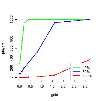
Figure 6. Owners by group with six values of extra gain

Eleven strategies

5.7
The third variation of the model explores a richer arrangement, trying to find out the best strategy for the first model. This model has agents following eleven distinct mixed strategies: s 0.0, s 0.1, …, s 1.0. The other parameters are the same as in M 0. Therefore we have the following model: M 11 = (C, 2, { E, ∼E }, u, { s 0.0, s 0.1, …, s 1.0}, s, 1200, 200, 20).

5.8
Figure 7 depicts the result of one experiment. In Figure 7(a) we can see that all strategies start with a similar number of cells, but quickly the ownership changes. In Figure 7(b) we can see that successful strategies in the first turns do not necessarily end the model with a high number of cells, as also shown in M 0. Some strategies are noteworthy. Agents that never escalate ( s 0.0) quickly own half the number of cells, shown in the peak of Figure 7(b). However, as the model evolves, they lose most of them and, when the model finishes, they place at the 7 th position. Equilibrium agents are quite successful, but they finish the model in the third position. The second place belongs to s 0.3, and the strategy that achieves the best result is s 0.2.

Figure
Figure 7a. Results of a single run with eleven strategies: a) Owners in the first 15 turns

Figure
Figure 7b. Results of a single run with eleven strategies: b) Owners along the simulation

5.9
Figure 8 summarizes the cells each group owns. The red line points out the maximum number of cells each group has achieved among all turns of all simulations. The blue line shows the cells owned by each strategy at the end of the simulations, with mean and standard deviation. The strategy s 0.0 has reached a maximum of 366 cells, and this value was omitted to give more emphasis to the other strategies. Note that the final ownership is similar to a gamma distribution. Also, there is no conflict in identifying the place of each group using the standard deviation as error, unless for groups from s 0.7 to s 1.0, which have achieved almost no cells.

Figure
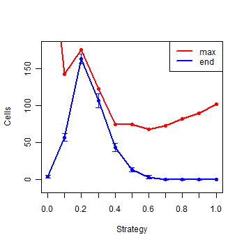
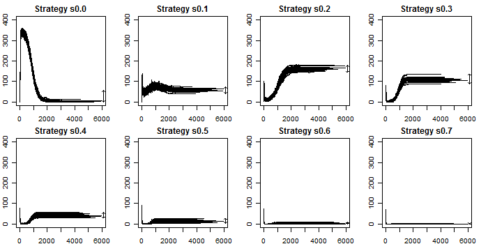
Figure 8. Summary of the eleven strategies at the end of the simulations

5.10
We can roughly divide the simulation in three stages. In the first stage, from the 1 st to the 5 th turn, the aggressive strategies ( s 0.5 to s 1.0) dominate the model and share the majority due to their initiative. The second stage emerges rapidly because they destroy themselves, making the purely cooperative strategy ( s 0.0) arise until it reaches the majority around turn 20. Finally, in the third stage, when most of the aggressive agents have already left the model, the more successful strategies slowly but ceaselessly conquer the cells dominated by s 0.0 agents. But, in the end, some cooperative agents still remain. They can only survive due to the possibility of having empty cells, as described in the results of M 0. The behaviour of such an agent consists in waiting until the simulation ends or someone forces it to leave the cell. Although this strategy can be considered naïve, the results show that this cooperative behaviour is nevertheless better than all the four more defective strategies ( s 0.7 to s 1.0), and it almost draws with s 0.6.

5.11
The individual development of each strategy in all simulations is shown in Figure 9. The groups from s 0.8 to s 1.0 have a development similar to s 0.7. We can see that each strategy has similar results in all simulations. In the right part of each graphic, there is a vertical arrow showing the maximum and minimum number of agents of each strategy at the end of the simulations. Note that, in all strategies but s 0.0, the higher and lower points of the arrow match the maximum and minimum number of cells achieved by those strategies. Although there is an average of only 3 cells owned by s 0.0 at the end of the simulations, there are 12 agents in these cells, thus 4 times the number of cells owned by the group. Strategy s 0.0 is the only one that supports more agents than cells, something that may happen only within a purely cooperative behaviour, because agents of other strategies end up by escalating sometime as the simulation progresses. Therefore, when we talk about surviving instead of owning, this strategy gains one more position, surpassing s 0.6 and almost drawing with s 0.5. Thus, there is not much difference between never escalating and acting without any strategy ( s 0.5), but it is better acting cooperatively than to adopt a tendency to escalate more often than not to escalate.

Figure
Figure 9. Ownership of strategies along all simulations

5.12
The majority achieved by s 0.2 and the second place achieved by s 0.3 can be explained by the result of Minf, which states that, as an agent escalates more, it can realise a threatening arrangement earlier. The counterpart of escalating more is the higher destruction of agents within the same group. Nash equilibrium is the base for a stable relation, and it can be used as a starting point for the best strategy. In this model, the best strategy uses the equilibrium, but it adds some risk to get more mobility. The winning strategy mixes both characteristics; its agents are not exploited by threatening agents and can conquer cells from s 0.0 faster than equilibrium agents.

* Conclusions

6.1
The results of the experiments show that changing parameters of the model that affect the mobility of the agents can lead to the success of strategies away from Nash equilibrium. The results show that risky agents take more advantage of the space, because they realize unfavourable arrangements earlier. But it may have a drawback of destructing players within the same strategy, which leads the strategy to be penalized as a whole. Therefore there exists a new equilibrium between these two factors. The evidence for this conjecture is shown in the results of M 11, presented in Section 5. In this model, there are eleven different strategies competing for space through a game with s 0.1 as equilibrium strategy, and the more successful strategy was s 0.2, winning each of the 50 runs. Although we do not expect the agents to be rational within this environment, Nash equilibrium is a good basis for the best strategy.

6.2
In all the models but the last one, there is not any grouping of agents at the end of the simulation because, if that occurs, the simulation has not ended yet. However, in the last variation of the initial model, it is possible to have more than one agent within each cell because we have one strategy that will never shoot ( s 0.0). This leads to groups of agents following this purely cooperative strategy within the same cell, increasing the number of agents following this strategy at the end of the simulations.

6.3
Clearly, the models can be enhanced with further refinements and sensibility analysis. For example, all the models presented in this article have agents homogenously distributed over the cells. In experiments not presented here, we studied models with the agents randomly distributed over the cells at the beginning of the simulation. The results are similar to the homogeneous case, with a straightforward increase on the standard deviation of the results, because there is a fourth stochastic ingredient, besides the escalating decision, the confronts, and the movement. We also tested the model using four neighbours by cell and found similar results. In fact, these results have the same explanatory power as the models presented in this work.

6.4
We can cite some questions to be investigated in future works. An open issue is to explore evolutive models concerning population dynamics. New populations are generated from the fittest agents of the previous simulation, with some mutation in their characteristics. Will these populations competing for space evolve to Nash equilibrium? Perhaps, "we can only expect some sort of approximate equilibrium, since […] the stability of the average frequencies will be imperfect" (Nash 1950). Another question that can be investigated is the evolution of cooperation within the context of mobility. Clearly a pacific agent does not need to wait until losing $20 since it arrived at the cell to move to another cell. Therefore we would have a more complex model, with the behaviour of agents differing not only by their mixed strategies, but also by their different ways to decide their actions based on the previous results. Within this environment, it is possible to investigate how the parameters of the model can affect how agents are grouped or repelled spatially, and the path taken by the different strategies.

* Availability

7.1
The model presented in this work was implemented in the TerraME modelling framework (Carneiro 2006). TerraME is a development environment for spatial dynamical modelling that links cell spaces to geospatial databases for data storage and retrieval. It uses the geoprocessing library TerraLib for working with geospatial data (Camara et al. 2000), and Lua language to create models (Ierusalimschy 2003). Because of its simplicity, Lua has a large number of programmers in the game development community, an activity that has many requirements in common with social simulation. The source code as well as the programs necessary for running the simulation are available at http://lucc.ess.inpe.br/doku.php?id=papers:mobility.

* References

AXELROD, R. (1980), 'Effective Choice in the Prisoner's Dilemma', Journal of Conflict Resolution, 24 (1), 3-25.

BELTRAN, F. S., SALAS, L., and QUERA, V. (2006), 'Spatial Behavior in Groups: an Agent-Based Approach', Journal of Artificial Societies and Social Simulation, 10.

BIELY, C., DRAGOSITS, K., and THURNER, S. (2007), 'Prisoner's dilemma on dynamic networks under perfect rationality', Physica D, 40-48.

CAMARA, G., et al. (2000), 'TerraLib: Technology in Support of GIS Innovation', II Brazilian Symposium on Geoinformatics, GeoInfo2000 (São Paulo).

CARNEIRO, T. G. S. (2006), 'Nested-CA: a foundation for multiscale modeling of land use and land change', (INPE, Brazil).

CASSAR, A. (2007), 'Coordination and cooperation in local, random, and small world networks: Experimental evidence', Games and Economic Behavior, 58, 209-30.

DURAN, O. and MULET, R. (2005), 'Evolutionary prisoner's dilemma in random graphs', Physica D, 208 (3-4), 257-65.

EPSTEIN, J. M. (1997), 'Zones of Cooperation in Demographic Prisoner's Dilemma', Complexity, 4 (2), 36-48.

FELDMAN, B. and NAGEL, K. (1993), 'Lattice Games with Strategic Takeover', in D Stein and L. Nadel (eds.), Lectures in Complex Systems, Papers from the summer school held in Santa Fe (5: Addison-Wesley), 603-14.

FERRIÈRE, R. and MICHOD, R. E. (2000), 'Wave Patterns in Spatial Games and the Evolution of Cooperation', in U. Dieckmann, R. Law, and J. A. Metz (eds.), The Geometry of Ecological Interactions: Simplifying Spatial Complexity (Cambridge University Press), 318-36.

IERUSALIMSCHY, R. (2003), Programming in Lua (Lua.Org).

KOSMIDIS, K., HALLEY, J. M., and ARGYRAKIS, P. (2005), 'Language evolution and population dynamics in a system of two interacting species', Physica A, 353, 595-612.

LE GALLIARD, J, FERRIÈRE, R., and DIECKMANN, U. (2003), 'The Adaptive Dynamics of Altruism in Spatially Heterogeneous Populations', International Journal of Organic Evolution, 57 (1), 1-17.

MANSURY, Y., DIGGORY, M., and DEISBOECK, T. S. (2006), 'Evolutionary game theory in an agent-based brain tumor model: Exploring the `genotype-phenotype' link', Journal of Theoretical Biology, 238, 146-56.

MAYNARD SMITH, J. (1982), Evolution and the Theory of Games (Cambridge University Press).

NASH, J. (1950), 'Non-cooperative games', (Princeton University).

NASH, J. (1951), 'Non-cooperative games', Annals of Mathematics (54), 286-95.

NOWAK, M. A. and MAY, R. M. (1992), 'Evolutionary Games and Spatial Chaos', Nature, 359, 826-29.

NOWAK, M. A. and SIGMUND, K. (1993), 'A strategy of win-stay, lose-shift that outperforms tit-for-tat in the Prisoner's Dilemma game', Nature, 364, 56-58.

NOWAK, M. A. and SIGMUND, K. (2000), 'Games on Grids', in U. Dieckmann, R. Law, and J. A. Metz (eds.), The Geometry of Ecological Interactions: Simplifying Spatial Complexity (Cambridge University Press), 135-50.

NOWAK, M. A., MAY, R. M., and SIGMUND, K. (1995), 'The Arithmetics of Mutual Help', Scientific American, 272 (6), 76-81.

OHTSUKI, HISASHI and NOWAK, MARTIN A. (2006), 'The replicator equation on graphs', Journal of Theoretical Biology, 243 (1), 86-97.

SCHEURING, I (2005), 'The iterated continuous prisoner's dilemma game cannot explain the evolution of interspecific mutualism in unstructured populations', Journal of Theoretical Biology, 232, 99-104.

SIGMUND, K (1993), Games of Life (Oxford University Press).

SOARES, R. O. and MARTINEZ, A. S. (2006), 'The geometrical patterns of cooperation evolution in the spatial prisioner's dilemma: an intra-group model', Physica A, 369, 823-29.

VAINSTEIN, M. H. and ARENZON, J. J. (2001), 'Disordered Environments in Spatial Games', Physical Review E, 64.

VUKOV, J. and SZAB, G. (2005), 'Evolutionary prisoner's dilemma game on hierarchical o lattices', Physical Review E, 71.

WU, Z. X., et al. (2006), 'Evolutionary prisoner's dilemma game with dynamic preferential selection', Physical Review E, 74.

ZHANG, J. (2004), 'Residential segregation in an all-integrationist world', Journal of Economic Behavior & Organization, 54, 533-50.

----

ButtonReturn to Contents of this issue

© Copyright Journal of Artificial Societies and Social Simulation, [2009]