Ravi Bhavnani, Dan Miodownik and Jonas Nart (2008)

REsCape: an Agent-Based Framework for Modeling Resources, Ethnicity, and Conflict

Journal of Artificial Societies and Social Simulation vol. 11, no. 2 7
<https://www.jasss.org/11/2/7.html>

For information about citing this article, click here

Received: 07-Nov-2007    Accepted: 18-Feb-2008    Published: 31-Mar-2008

Abstract

This research note provides a general introduction to REsCape: an agent-based computational framework for studying the relationship between natural resources, ethnicity, and civil war. By permitting the user to specify: (i) different resource profiles ranging from a purely agrarian economy to one based on the artisanal or industrial extraction of alluvial or kimberlite diamonds; (ii) different patterns of ethnic domination, ethnic polarization, and varying degrees of ethnic salience; as well as (iii) specific modes of play for key agents, the framework can be used to assess the effects of key variables — whether taken in isolation or in various combinations — on the onset and duration of civil war. Our objective is to make REsCape available as an open source toolkit in the future, one that can be used, modified, and refined by students and scholars of civil war.

Keywords:

Agent-Based Model, Ethnicity, Salience, Polarization, Domination, Civil War, Greed, Natural Resources

Introduction

1.1

The onset of civil war is influenced by a set of processes that interconnect political, economic, and social factors, a prime example of a complex adaptive system, in which many decision-making agents, each with their own characteristics and behaviors, interact with and change both the physical environment and other agents, leading to nonlinear and path-dependent dynamics.¹

1.2

Work on the resource-conflict link was popularized by Collier and Hoeffler (1998 ; 2004; 2005), who found that greed-based incentives for rebellion were likely to dominate in countries with significant natural resource deposits, in contrast to earlier research in political science which emphasized the primacy of ideological or grievance-based incentives for rebellion. Collier and Hoeffler's (CH) work generated a veritable cottage industry of research, beginning with work that replicated CH's findings using different data sets. Not unexpectedly, this body of research produced mixed results, due largely to the use of dissimilar data, distinguished by the diversity of coding criteria for conflicts, measurement and operationalization of key explanatory variables, and procedures for coping with missing data.² As such, these findings both reinforced (Buhaug and Gates 2002; Doyle and Sambanis 2000; Hegre 2002; Humphreys 2005) and undermined (Fearon and Laitin 2003; Elbadawi and Sambanis 2002) CH's propositions on the resource-conflict relationship.³

1.3

As part of this research program, scholars have attempted to assess the impact of ethnicity on the incidence of civil wars. This endeavor has generated ongoing theoretical (and methodological) disagreements. On the one hand, scholars argue that ethnicity - ethnic fractionalization, polarization, and domination - plays a significant role in motivating individuals to initiate and/or participate in insurgency (Cederman and Girardin 2007; Elbadawi and Sambanis 2002; Gates 2002; Hegre and Sambanis 2006; Lujala et al. 2005; Sambanis 2001; Wimmer et al. 2007). In contrast, others suggest that ethnicity is at best secondary to economic and other material considerations that motivate individuals to rebel (Collier and Hoeffler 2004; Fearon et al. 2007; Fearon and Laitin 2003; Montalvo and Reynal-Querol 2005; Reynal-Querol 2002; Ross 2004). The mechanisms underlying ethnically based support of governments or rebels, remain largely unpacked.

1.4

Multivariate statistical models exploring the significance of these key variables in civil wars have established empirical regularities (Hegre and Sambanis 2006; Sambanis 2001) although these studies are constrained by the use of different measures of ethnicity and natural resource wealth, as well as in their ability to specify underlying causal mechanisms given: (i) the large number of relevant causal factors; (ii) complicated interactions between agents and associated factors; (iii) the difficulty of collecting useful data on agent characteristics and behavior; (iv) a limited set of "natural experiments" to test the effects of varying factors.⁴ Moreover, the very characteristics of complex adaptive systems - agent heterogeneity and adaptation, nonlinear mechanisms and feedback loops, non-random interaction topologies, and non-linear, path dependent dynamics - violate many of the assumptions underpinning the use of traditional large-N approaches. In the absence of adequate tools to deal with complex behavior, researchers are inclined to ignore these complexities, unnaturally limiting the scope of social research (Meyer et al. 2005).

1.5

One approach that is well suited to meeting the challenge of modeling a complex adaptive system is agent-based modeling (Bankes 2002; Bonabeau 2002; Conte et al. 1997). In short, when a system is complex, our unexamined, first intuitions are often insufficient. Because ABMs are computational models, they are formal, unambiguous and thus replicable and testable (Axelrod 1997; Axelrod and Cohen 2001), lending themselves to study aspects of complex systems that are difficult to study using traditional analytic techniques (Parunak et al. 1998).

1.6

Our objective in this essay is to describe the building blocks of an exploratory ABM framework entitled REsCape (for Resources, Ethnicity, and Conflict) that serves as an experimental device, while stopping short of offering precise and detailed forecasts.⁵ REsCape permits the user to select different degrees of ethnic salience, patterns of ethnic polarization and domination, resource profiles, and agent strategies to determine how these factors could influence the incidence of civil violence. Given the multiplicity of explanatory factors we have strayed, albeit reluctantly, from the KISS principle.⁶ As such, REsCape is sufficiently complex - in so far as it captures key economic relationships such as investment, depreciation, taxation, extraction and the generation of revenue; includes standard conflict success functions; operationalizes prevalent conceptualizations of ethnicity; and utilizes commonly adopted measures of conflict onset and duration - yet sufficiently transparent in that it enables the user to identify key causal drivers under a given set of initial conditions.

1.7

We believe REsCape may be used both as a general tool to study the potential relationship between the key explanatory variables listed above and the incidence of civil war, or be tailored to fit the specifics of a given case. In ongoing research, we utilize REsCape to address extant arguments in the civil war literature, such as the link between ethnic polarization, economic growth, and civil war (see Bhavnani and Miodownik 2008a), as well as the impact of ethnic minority domination on conflict risk (see Bhavnani and Miodownik 2008b). Our ultimate objective is to make REsCape available as an open source toolkit, to be modified and refined by the community of scholars interested in the use of ABM to understand the causes, underlying mechanisms, and trajectories of civil war.

REsCape: An Agent-Based Computational Framework

2.1

Figure 1 presents a summary of key model components (1 - 9), mechanisms (a - d), and feedback loops (i - n). To begin with, we define a landscape (1) as a discrete cellular grid with fixed borders, and a capital city (C) located in the center.⁷ We note that the size and the shape of this grid is alterable by the user. In the current specification, each of the 441 (21×21) cells may contain any number of agents, divided into members (peasants) and leaders of two rival ethnic groups (2).

---

Figure 1. REsCape - Summary of Key Model Components and Mechanisms

---

2.2

The landscape is characterized by production which falls into one of four economic sectors (3). Sectoral and spatial spending decisions (4) by leaders of each ethnic group determine the amount of revenue (5) available to garner peasant support (6). Where such support is weak, peasants may relocate or migrate (7) to cells populated and controlled by members of their own ethnic group. Revenue is also used by leaders to control territory (8), and we underscore the importance of territorial control in this framework, given that control is a necessary condition for spending and investment, revenue generation, and popular support. All control is cell-specific, as is the breakdown of economic sectors, spending decisions, and peasant support. Conflict (9), also cell-specific, emerges when group leaders seek to control the same territory or cell. Specific mechanisms include the following: (a) robbery leads to a decline in economic growth, undermining peasant support and weakening the state, making it more vulnerable to capture over time; (b) spending on social welfare increases popular support, but remains economically unviable in the long-term; (c) spending on coercive power alters support and is essential for territorial control; and (d) investment in the economy serves to increase the flow of revenue over time, and has a robust effect on peasant support. Key feedback loops in the framework include the following: (i) changes in revenue (relative to the revenue of nominal rivals) increase (or decrease) the salience of ethnicity; (j) ethnic salience affects peasant support; (k) high levels of peasant support decrease the cost of control, and control has a non-monotonic effect on support (excessive control lowers support, as does weak or insecure control); (l) when peasant support for the leader in control of a cell is weak, peasants may exercise the option to migrate to ethnic enclaves, in an effort to find safety in numbers; (m) migration changes the calculus of control, and thus affects spending, investment, and support for leaders; (n) conflict, which arises when leaders seek to control the same territory, alters the control of individual cells and may ultimately alter control of the state (the ethnic group in power or the EGIP).

2.3

We describe the basic sequence of model steps below:

• Determine the resource base and spatial distribution of resources in the economy
• Determine the strategy defining spending and investment decisions on the part of group leaders
• Determine the degree of ethnic polarization by specifying the population share of rival ethnic groups
• Determine the structure of ethnic domination by specifying the EGIP and by default the EGOP
• Determine whether ethnic salience is fixed or variable
  
  • In each timestep of a model run:
  • • Group leaders make sectoral and spatial spending decisions
    • Spending decisions generate revenue for leaders and peasants
    • Future spending and investment is, in turn, constrained by revenue
    • Peasants determine their level of support for leaders as a function of revenue, security, and ethnicity
    • If support is low, peasants migrate to ethnic enclaves
    
    
  • Conflict emerges when group leaders seek to control the same cell
  • • Conflict determines new patterns of territorial control
    • Change in control of the capital city effectively changes the EGIP

2.4

In the paragraphs that follow, we present a more detailed description of the model's building blocks and relegate additional detail to the Appendix.

Ethnicity: Identity, Salience, and Polarization

2.5

All agents carry an ethnic marker identifying them as members of an ethnic group A or B, with the leader of the EGIP denoted by Ȧ and the leader of the EGOP denoted by Ḃ.⁸ We refer to all non-leader agents as peasants P. Ethnic salience e denotes the significance of ethnicity to a peasant, and may either be fixed (e_i^Ȧ = e_i^Ḃ = 1) for all peasants or vary across peasants (e_i^Ȧ, e_i^Ḃ,∈ [0,1]). In the latter case, we specify ethnic salience as a function of relative revenue: the greater the disparity between a peasant's per capita income and the income of nominal rivals, the greater the salience attached to her ethnicity (we provide additional detail for this calculation in the Appendix). Levels of ethnic polarization, the probability that two randomly selected peasant's will belong to different ethnic groups weighted by the relative size of each group, may be specified by the user, as may the structure of ethnic domination, i.e. the group in control of state power.

The Economy: Revenue, Spending, and Support

2.6

The model's landscape is comprised of individual cells, each of which may host one of the four productive sectors: agriculture ag; artisanal alluvial diamonds aa; industrial alluvial diamonds ai; and industrial kimberlite diamonds ki.⁹ In this section, we provide a general description of the model economy, and leave the sector specific details to the Appendix. To begin with Ȧ,Ḃ decide how much to invest in each cell under their control, with investment raising the amount of extractable revenue in the short-run and increasing overall productivity and revenue in the medium to long run. Revenue generated by each sector x in a grid cell is allocated to the actor in control of the cell Ȧ, Ḃ and the peasants in the cell P in the following manner:

where s_x ∈ [0,1] denotes the share of revenue going to the controlling agent.

2.7

A sectoral and spatial spending strategy determines the share of revenue Ȧ,Ḃ allocates to (i) coercive power, (ii) robbery, (iii) economic investment, and (iv) social welfare payments to peasants, as well as the distribution of revenue across cells in the landscape.¹⁰ A control strategy determines which cells on the landscape Ȧ,Ḃ seek to control, as well as the distribution of coercive power over these cells, as a function of the cell's (i) resource base, (ii) peasant population, (iii) distance to capital, (iv) proximity of other cells under the agent's control. The combination of spending and control strategies yield a set of stylized "modes of play" for Ȧ,Ḃ :

• Robbery is a "predatory" strategy in which leaders maximize personal profit by appropriating tax revenue from the economy, while neglecting further investment and relinquishing control of unprofitable areas.
• Social Welfare is a "populist" strategy designed to increase peasant support through high levels of social spending.
• Territorial Control is a "militant" strategy in which spending on coercive power to increase and/or maintain physical control over territory is paramount.
• Benevolent Rule is an "ideal" strategy in which leaders balance investment in the economy with spending on coercive power and social welfare.

2.8

Next, we define a measure of peasant support s^P for the "accountable agent" i.e. the leader in control of a given cell (note that support need not be limited to leaders of one's own group, and that accountability is limited to leaders alone). This measure ranges from -10 to +10 (where -10 denotes total support for leader Ḃ, +10 denotes total support for leader Ȧ, and 0 denotes neutrality) and depends upon: (i) current revenue; (ii) changes in revenue over time; (iii) the coercive power of the "accountable agent"; and (iv) the ethnicity of the "accountable agent". Specifically, we take the difference between actual revenue y^P and a reference revenue y_ref ^P and the difference between y^P and the past revenue y_past^P. Let y_past^P be weighted sum of past revenue:

y_past^P(t + 1) = k_ws y_past^P(t) + (1 - k_ws) y^P(t)

where k_ws ∈ [0,1] represents the "length" of memory. It follows that as k_ws decreases, the rate at which a peasant "forgets" the past increases. We then specify a function h(c^a) which describes how peasant support is affected by the coercive power c^a of the leader in control of a cell, such that h(c^a) begins at -1 for no coercive power, rises linearly to +1 for c^a = c_ideal, falls linearly to -1 for c^a = c_oppressive, and remains at -1 for c^a ≥ c_oppressive. This function is then weighted by a parameter k_CP. Lastly, support is affected by ethnic salience, such that if e_i>0 then k_e equals -1 if the peasants and leader are from different groups, 1 if the peasants and leader are from the same group, and 0 if e_i < 0.¹¹ Adding these terms, and inserting them into a logistic function yields:

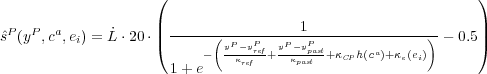
where equals -1 for Ḃ, +1 for Ȧ, and 0 otherwise. The update rule for s^P(t) is:

where λ_s captures the "inertia" or the rate at which a peasant adapts her sympathy to changes in economic well being.

2.9

Finally, peasants may move or migrate to "ethnic enclaves" using the following rules:

• For peasant i, every x_i timesteps,
  
  • IF Ȧ controls the cell AND IF s^P < 5 THEN max over mobility radius m
  • IF Ḃ controls the cell AND IF s^P > -5 THEN max over mobility radius m

2.10

That is, if s_i^P falls below 5 (-5), then peasant i will move a maximum distance m to a cell with the greatest number of co-ethnics n_A(n_B), and highest degree of control q_c^Ȧ(q_c^Ḃ) exercised by a leader from the peasant's ethnic group. The migration of peasants has implications for control, given that high levels of peasants support lower the cost of control, whereas this cost increases in the absence of strong support.

Conflict: Coercive Power, Control, and Civil War

2.11

Coercive power c is cell- and leader-specific, updated every timestep by new investment i_c, depreciation δ_c (to reflect the normal wear of equipment and attrition), and loss l incurred as a result of conflict, and change in the density of "ethnicized" φ_e^p peasants (the number of peasants for whom ethnic salience e equals 1):

2.12

Control q_c ∈ [-10,10] is a function of the average peasant support in the cell ( ^P), the coercive power (c^Ȧ and c^Ḃ) of leaders in the cell, and the cell's distance from the capital city, with -10 denoting complete control by Ḃ of a cell and +10 denoting complete control by Ȧ of a cell.

2.13

Conflict occurs when Ȧ,Ḃ seek to control the same cell, given that control is necessary for investment and profit. Specifically, conflict occurs when the coercive powers of both Ȧ,Ḃ in a cell exceed a threshold τ_c, with loss l proportional to the magnitude and outcome of the conflict, such that:

where f ∈ [0,1] is the conflict outcome variable (f = 1 being total victory by Ȧ and f = 0 total victory by Ḃ), c_sum = c^Ȧ + c^Ḃ is the sum of all coercive powers involved in the fight, and α is a parameter that determines the intensity of conflict (by scaling the losses). We define the conflict outcome variable f using the log-ratio of coercive power log , measuring control in cells surrounding the conflict q_sur = ∑ _iM q_cⁱ (where M denotes the conflict cell and its Moore Neighbors, q_cⁱ denotes control in cell i), using a distance function , and introducing a stochastic term X ~ N(0,σ²) where σ² is the amount of randomness we seek to introduce. Taking the sum of these terms in the logistic function yields:

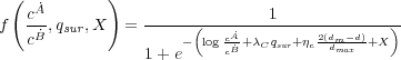
where λ_c weights the influence of control in surrounding cells, and where η_c weights the influence of the geography. Control of the cell under contention shifts to the victorious agent, and in the case of widespread conflict, may result in a change of the EGIP.

Demonstration Run and Descriptive Results

3.1

In this section, we describe two baseline model runs. In the first of the two runs, we document the effect of a change in the government's strategy from benevolent to robbery in an alluvial diamond economy where all peasants belong to the same ethnic group, and discontented peasants rebel against the government. In the second demonstration run, we introduce ethnicity with the majority group A constituting the EGIP and hold all else constant.

---

Figure 2. Demonstration Run I Screenshots Note: The demonstration was run with the following parameters settings: all agents belong to the same ethnic group (A); government strategy (t ≤ 150) = benevolent; government strategy (t > 150) = robbery; rebel strategy = benevolent; resource base = alluvial; resource location = point source. The text that follows describes the screenshots in the figure. ROW 1 (white, green. black): the brighter the color of a cell, the higher the priority accorded to the cell by the government; white cells reflect a high priority, followed by deepening shades of green (decreasing priority) which merge into black (a lack of interest in the cell). ROW 2 (greyscale): the brighter the cell, the higher the population density of the cell; white cells are heavily populated, grey cells are moderately populated, whereas black cells are not populated; magenta dots indicate the presence of alluvial diamond deposits within a cell. ROW 3 (green, blue, black): green cells denote peasant sympathy in favor of the government; blue cells denote peasant sympathy in favor of the rebels; black cells denote neutrality. ROW 4 (greyscale): the brighter the cell, the higher the level of government coercive power in the cell; white cells indicate a significant troop presence; grey cells a moderate presence; and black cells the absence of any government troops. ROW 5 (green, blue, black, red): green cells denote government control; blue cells denote rebel control; the brighter the color, the greater the extent of control; red indicates that conflict over control of the cell has erupted. ROW 6 (black, red): a cell colored red at timestep t* indicates that there has been at least one conflict in the cell at time t < t*.

---

Demonstration Run I

3.2

In the first demonstration run of the model, the government plays a benevolent strategy (and later switches to robbery), the rebels play a benevolent strategy, and all peasants belong to the same ethnic group. The landscape we utilize for the demonstration is characterized by high population density in the center, moderate density in the NW, NE, and SE corner regions, and low density in the remaining areas, and contains alluvial diamond deposits located in a ring around the capital city.

3.3

Priming the Model (timesteps 0-149)¹². During the first 149 timesteps, we prime the model with the baseline benevolent government strategy, which results in complete government control of the landscape, high revenue from industrial mining of alluvial deposits and taxation of agriculture, and a peasant population that fully supports the government. In addition, this period is marked by the absence of conflict, as depicted in the screenshots in Figure 2. In addition to these screenshots, Figures 3-6 provide details on the amount and sources of government revenue, number of ongoing conflicts in the landscape, proportion of cells affected by at least one conflict, and number of cells under government and rebel control.

3.4

Switching the Government's Strategy: From "Benevolent" to "Robbery" (steps 150-200). At timestep 150, we alter the government's strategy to robbery, a "predatory" strategy in which leaders appropriate revenue from the economy for personal use, neglect investment, and relinquish control of all unprofitable cells. The government's control strategy display indicates that the change in strategy effectively makes large portions of the landscape unappealing to the government. Only the densely populated center, NW, NE, and SE corners, and diamond sites remain important enough to warrant the government's deployment of coercive power. By timestep 200, the following developments occur: (i) government agricultural revenue falls dramatically (See Figure 3) due to greater robbery and thus lower investment, as evidenced by the marked increase in the leader's level of personal consumption; (ii) peasant sympathy for the government decreases, due primarily to lower income from agriculture, although government revenue from alluvial diamonds remains high; (iii) peasant sympathy for the government at diamond sites, where peasants still enjoy high income from artisanal mining of alluvial diamonds, remains high; (iv) the government effectively exercises control along a corridor from the NW to the SE, although coercive power declines in other areas; (v) the decline in coercive power and peasant sympathy erodes the government's ability to control cells along the N and E edges, where rebellion begins to emerge.

3.5

The Growth of Conflict (timesteps 200 - 540). At timestep 540, the screenshots in Figure 2 depict the following changes: (i) a steeper decline in government revenue from agriculture and corresponding decline in government control; (ii) a rise in the number of cells controlled by rebels, with a commensurate rise in agricultural revenue captured by rebels; (iii) a marked increase in conflict in the SW and NE quadrants. In particular, the number of cells having suffered at least one conflict rises dramatically in this period, as the rebellion grows and reaches areas in which the government more fiercely defends itself. By the end of this period, rebels control areas with low population density, while the government retains control of the NW to SE corridor and valuable diamond sites. Rebel revenue consequently remains below government revenue.

3.6

The Spread of Conflict (timesteps 540 - 1720). This period sees a continuation of trends observed in the last period, with a few notable differences: (i) conflict onset increases significantly (after timestep 1400) in areas with diamond deposits (see Figures 4 and 5); (ii) rebel revenue increases significantly, with a commensurate increase in the severity of fighting; (iii) government revenue from alluvial diamond mining begins to decrease, as the government finds it increasingly difficult to sustain even the limited diamond economy; (iv) close to timestep 1400, the rebels begin their capture of diamond sites, and begin investing in artisanal mining;¹³ (v) by timestep 1720, government revenue begins to fall below rebel revenue, at which point the government is pushed back to the central region of the landscape, opening the path to a rebel victory.

3.7

Rebel Control (timesteps 1720 - 1920). In this period, the rebels continue to push the government back. Timestep 1920 captures the imminent fall of the government, after which the rebels assume control of the entire landscape (see Figure 6), and effectively become the new government.

---

Figure 3. Changes in Government and Rebel Revenue Over Time

---

Figure 4. Number of Ongoing Conflicts

---

Figure 5. Proportion of Landscape Affected by Conflict Onset

---

Figure 6. Number of Cells Under Government and Rebel Control

---

Demonstration Run II

3.8

In the second demonstration run, we introduce rival ethnic groups, with members of the EGIP A constituting 85% of the population and members of the EGOP B constituting 15% of the population. It follows that the dominant ethnic majority A exercises political control, whereas the minority group B is excluded from power. We also permit the salience of ethnicity to vary across peasants, who periodically shift their location on the landscape. Apart form these changes, we leave the government strategy unchanged - Ȧ plays a benevolent strategy (and later switches to robbery), and continue to utilize a landscape characterized by high population density in the center, moderate density in the NW, NE, and SE corner regions, and low density in the remaining areas, with alluvial diamond deposits located in a ring around the capital city. We also leave Ḃ's strategy unchanged. The screenshots in Figure 7 capture changes in strategy and control, peasant population density and sympathy, ethnic salience and the formation of ethnic enclaves, and conflict for each of the periods discussed below.

---

Figure 7. Demonstration Run II Screenshots Note: The demonstration was run with the following parameters settings: agents belong to rival ethnic groups (A,B); EGIP = A, EGOP =B; Ȧ 's strategy (t ≤ 150) = benevolent; Ȧ 's strategy (t > 150) = robbery; Ḃ 's strategy = benevolent; resource base = alluvial; resource location = point source; nA = 0.85 ; eiA,eiB, [0, 1] with "per-capita range" = 3; ethnic group in power = A; migration period xi(min,max) = (25,200). The text that follows, describes the screenshots in the figure. ROWs 1-5 (See caption for Figure 1). ROW 6 (Green, Black): green cells denote ethnic salience for members of group A; the brighter the color, the greater the salience of ethnicity. ROW 7 (Green, Black): green cells denote the location of members of group A; the brighter the color, the greater the density of A's. ROW 8 (Blue, Black): blue cells denote ethnic salience for members of group B; the brighter the color, the greater the salience of ethnicity. ROW 9 (Blue, Black): blue cells denote the location of members of group B; the brighter the color, the greater the density of B's. ROW 10 (black, red): a cell colored red at timestep t* indicates that there has been at least one conflict in the cell at time t < t*.

---

3.9

Priming the Model (timesteps 0-149). The first 149 timesteps, which constitute the baseline period, are characterized by high levels of agricultural revenue and the absence of violence. Migration levels are moderate, with peasants moving to cells characterized by greater numbers of ethnic kin and control exercised by members of their own ethnic group. For members of minority group B, migration results in the formation of enclaves towards the edges of the landscape, given that government control is weakest here. In contrast, members of majority group A begin to cluster around the central mining region. Despite this ethnic clustering, overall levels of sympathy favor the government.

3.10

Switching Ȧ's Strategy: From "Benevolent" to "Robbery" (steps 150-200). The transition in Ȧ's strategy rapidly generates a shift in peasant sympathy, which now begins to favor Ḃ in ethnically heterogeneous cells in which the mode of production is predominantly agricultural. In the central, diamond-rich region, however, sympathy for Ȧ remains high. Of note is that the newly formed minority enclaves tend to be located at such great distance from the majority-controlled resource-rich regions, that comparisons of per capita income fail to generate grievances on the part of the minority, resulting in levels of sympathy that are largely neutral, in so far as they favor neither Ȧ nor Ḃ.

3.11

The Growth of Conflict (timesteps 200 - 540). By timestep 400, conflict begins to occur in ethnic enclaves within "per-capita range" (see our explanation in the Appendix) of diamond deposits, where the income differential between nominal rivals increases the salience of ethnicity, undermines support, and results in flight by the more privileged members of group A, and the subsequent occupation of abandoned territory by members of B.

3.12

The Diminution of Conflict (timesteps 540 - 1720). By timestep 1000, a large minority enclave has formed along the southern edge of the landscape. As this enclave grows in size, it becomes home to nearly all members of B, pushes members of A out of "per-capita range", and weakens Ȧ's control. As ethnic homogeneity increases in this enclave, both ethnic antagonism and violence subside.¹⁴

3.13

The Reassertion of Government Control (timesteps 1720 - 1920). Ethnic clustering stabilizes by timestep 2000, with unrest limited to isolated pockets of majorities in the minority dominated southern enclave, and isolated pockets of minorities in the majority dominated northern enclave. Over time, even these isolated pockets disband, as peasants migrate to find safety in numbers. Moreover, with its control of diamond deposits secure, Ȧ's ability to quell unrest in the north remains high, resulting in the eventual elimination of conflict and the close to complete segregation of peasants along ethnic lines.

3.14

The two demonstration runs provide a practical description of the framework, its major components, mechanisms, and feedback loops. Clearly, our limited analysis in this research note is not intended to explore the effect of key variables on the incidence of civil war, but rather, to serve as an introduction to REsCape.

Conclusions

4.1

REsCape incorporates key variables such as ethnicity, polarization, dominance, resource type, and agent behavior into a formal computational model which can be used to address the ongoing debates engaging students of civil war. The framework permits the user to conduct complicated thought experiments, experiments for which empirical data would be difficult to collect. For instance, users interested in the behavior of key agents could explore how a ruler's ability to generate revenue through the taxation or looting of natural resources could affect the onset and duration of civil war. Those interested in understanding the micro-foundations of rebellion could focus on the conditions under which the opportunity cost faced by peasants for joining a rebellion decrease. Those interested in studying the effects of ethnicity on the incidence of civil war could formally study the consequences of different conceptualizations of ethnicity, as well as different patterns of ethnic domination and polarization, or introduce new measures of ethnic salience beyond the basic measures the framework currently provides. Those interested in exploring the relationship between natural resources and conflict could examine the effects of ruler and rebel behavior under a variety of resource regimes and resource profiles. And those interested in studying conflict at the sub-national level could distinguish between events that comprise a particular conflict, such as the transfer of territory, capture of resource deposits, and capture of the capital city.

4.2

Table 1 presents a summary of key parameters in REsCape as well as the range of values these parameters may take. To summarize: leaders may adopt one of four stylized strategies; the resource base may vary from agriculture to one based on harder to extract kimberlite or artisanally extracted alluvial diamonds; peasants may be members of one of two ethnic groups with the salience they attach to their ethnicity varying, from the base case in which ethnicity is not salient, to the largely primordial conceptualization where ethnicity is salient for all individuals and always affecting their behavior, to variation across individuals and groups based on grievances that result from income disparity, calculated across a continuum ranging from the agents own cell to the entire landscape; finally, one may also seed the model to capture different patterns of ethnic polarization and domination.

4.3

We have only begun to explore a small fraction of the parameter space in REsCape, and it is inconceivable that any one paper could fully explore this space. That said, we conclude with a caveat: REsCape serves as an exploratory tool, not a comprehensive model intended to capture all the causes and dynamics associated with civil wars. As such, the framework may be extended in a number of directions: users may seek to assess the effect of transnational linkages on the incidence of civil war; choose to seed the model with GIS data to capture the geographical contours of particular real-world cases; analyze the effect of mixed strategies or endow agents with the capability to look ahead and modify their behavior in anticipation of their opponent's moves; or simplify the framework to focus on specific parameters of interest to the researcher. The policy significance of this toolkit should be apparent, in that it permits the user to conduct complicated thought experiments, or counterfactual analysis, that can be tailored to the specifics of a given scenario.

4.4

Our future development of REsCape may be summarized as follows: (i) add a GIS interface to utilize country or region-specific landscapes; (ii) develop additional resource profiles (oil, timber, water), agents (military, corporations), and strategies (leader-look ahead); (iii) collect empirical data to apply the framework to select real-word cases; (iv) develop the architecture to host an online release of REsCape which will serve as an open-source toolkit, to be used, modified, and refined by students and scholars of civil war. In our own research with REsCape, we explore the link between ethnic polarization, ethnic salience, and civil war, making the case of a more nuanced understanding of the effect of polarization on conflict (Bhavnani and Miodownik 2008a), and assess the extent to which minority domination affects the incidence of civil war under a variety of resource regimes and agent strategies (Bhavnani and Miodownik 2008b).

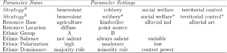
Table 1. Range of Experiments with REsCape

Note:

In the current version of REsCape, Ḃ is limited (*) to playing the benevolent strategy.

Appendix

A.1

This appendix provides additional details on select model components outlined in Section 2.

Ethnicity: Identity, Salience, and Polarization

A.2

We specify ethnic salience as a function of relative revenue: the greater the disparity between a peasant's per capita income and the income of nominal rivals, the greater the salience attached to her ethnicity. Let N equal the total population and let n_A denote the proportion of peasants from group A, n_B proportion from group B. Per capita income for members of group A is then defined by y_pc^A,r = , where r denotes the range over which per capita income is calculated, what we refer to as the "per-capita range", which can vary from 0 (only the current cell in which the peasant is located) to 10 (the entire landscape), permitting peasants to make "local" or myopic calculations, or by contrast, calculations based on "global" information. By a similar logic, per capita income for group B is given by y_pc^B,r = . Ethnicity becomes salient when a peasant's per capita income is smaller than the per-capita income of nominal rivals. It follows that for a member of group A, ethnic salience is give by e_i^A = , and by the same logic, the salience of ethnicity B would given by e_i^B = .

The Economy: Revenue, Spending, and Support

A.3

We define investment :

with sector-specific depreciation rates δ_ki, δ_ai,δ_aa and δ_ag ≤ 1. Every investment i₀ decays exponentially assuming continuous time and no further investment:

Note that investment in industrial production is constrained by an upper limit _max, such that _ki,max= μ_ki,max *k and _ki,max = μ_ai,max *a (where k and a respectively denote the size of kimberlite and alluvial deposits in a cell), and that a minimal level of investment _ki,min = μ_ki,min * k, = μ_ai,min* a is required to generate revenue. That is, we assume that minimum and maximum investment for the extraction of kimberlite diamonds exceeds that for alluvial diamonds, i.e. μ_ki,max > μ_ai,max and μ_ki,min > μ_ai,min, and that investment in industrial diamond production is limited to Ȧ, although Ḃ can profit from previous government investment when it assumes control of a cell. Note also that investment in artisanal and agricultural production is not bounded and does not require a minimum level to generate revenue.

A.4

Revenue generated by industrial (alluvial or kimberlite) production is given by:

where ρ is a constant that defines the yield from industrial production. Revenue generated by artisanal alluvial diamond production is given by:

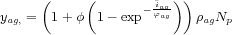
where ρ_aa is a constant defining the yield from artisanal alluvial production, N^P denotes the number of peasants in a cell, and a_aa = a - a_ai, with a_ai = . And lastly, revenue generated by agricultural production is given by:

and where ρ_ag is the productivity of the peasants, N^P denotes the number of peasants in a cell, φ is the maximum increase in productivity generated by investment, and φ_ag is a scaling factor that determines the requisite level of investment for a given level of revenue. Due to the highly organized and controlled process of diamond mining in industrial production, we assume that the leader in control is the sole recipient of revenue from all industrial production (s_ki = 1 and s_ai = 1). Turning to artisanal extraction and agriculture, we specify s_aa and s_ag as increasing with investment in each sector, and assume that in the absence of investment, the minimum share of revenue going to Ȧ,Ḃ is given by s_aa,min, s_ag,min, and the maximum share by s_aa,max, s_ag,max:

where and are scaling factors that determine the requisite level of investment for a given share. Note that while investment in the artisanal sector has no direct influence on total revenue, it does affect the ability of Ȧ,Ḃ to tax peasant revenue.

Sectoral Spending Decisions

A.5

The spending strategy determines the share of revenue allocated to: (i) the expansion of coercive power (i.e. military spending); (ii) personal consumption; (iii) investment in the industrial extraction of resources (kimberlite or alluvial) - a mode of production that is easier to tax; (iv) investment in artisanal alluvial extraction, harder to tax but preferred by Ḃ; (v) investment in agricultural extraction, which may provide a lower rate of return compared to other economic sectors; and (vi) investment in welfare payments to peasants. Table A1 depicts the parameter values selected to implement our strategy set. Note that β_c and β_r are defined by strategies, rather than the resource base. With respect to β_ki, β_ai, β_aa, β_ag, we note that every strategy has a base value for β_ag, and a base value for investments in diamond mining (β_ki for kimberlite diamonds and β_ai for alluvial diamonds). In the case of a purely agricultural resource base, investment intended for diamond mining is diverted to agriculture (on the row for "robbery (AG)", the value for β_ag is 0.8, or the sum of 0.5 allocated to agriculture and 0.3 allocated to diamonds).

Table A1. Agent Strategies

Note: This table summarizes the distribution of spending for each of the four stylized strategies. The leftmost column denotes the strategy name and (in parentheses) the resource base. The next two columns "terr control" and "robbery" denote the share of revenue allocated to coercive power and personal consumption or theft. Any remaining revenue is then invested in the economy according to the weights specified in the next five columns.

Spatial Spending Decisions

A.6

After allocating revenue across categories, a leader distributes these funds over grid cells by:

1. Assigning investment targets to every grid cell under his/her control:
   • In the kimberlite and alluvial industrial sectors, the target is the maximal investment allowed.
   • In the alluvial artisanal sector, the target is proportional to the size of deposits available for artisanal mining.
   • In the agricultural sector, the target is proportional to the number of peasants in the cell.
   • With respect to social spending, the target is defined as the desired level of peasant sympathy (-10 for Ḃ, +10 for Ȧ).
2. Distributing available funds in proportion to the difference between the targeted and the current level of investment in a cell

Conflict: Coercive Power, Control, and Civil War

A.7

The control strategy determines exactly which cells on the landscape Ȧ,Ḃ seek to control, as well as the distribution of coercive power over these cells, as a function of several cell specific characteristics. The first pertains to the existence of (kimberlite or alluvial) diamonds in the territory - in other words the expected revenue from extraction and taxation. Then there are characteristics of the population: whether a cell is densely populated, together with its ethnic composition. The third determinant of the control strategy is the distance from the capital, which imposes difficulties on government control, but facilitates insurgency or opposition. Lastly, Ȧ,Ḃ consider the proximity of a cell to cells already under their control. The strategy assigns a priority value v to every cell, based upon the following factors and associated weights given by γ :

• the existence of kimberlite/alluvial diamonds in the cell (γ_kim, γ_all)
• peasants population density (γ_N^P)
• peasant ethnicity (γ_e^p)
• distance from the capital (γ_cap,close, γ_cap,far)
• proximity of Ȧ,Ḃ controlled cells (γ_close^Ȧ, γ_close^Ḃ)
• average control value in the cell and neighboring cells is in favor of Ȧ,Ḃ (γ_q^Ȧ, γ_q^Ḃ)

A.8

Based on these factors Ȧ,Ḃ ignore cells whose priority value v is lower than a priority threshold τ and ignore all cells already under their own control. Specifically, Ȧ,Ḃ choose n cells with the highest priority value, and build-up coercive power in these and neighboring cells. Table A2 depicts the weights assigned to different factors for each agent strategy. Note that robbery and territorial control are characterized by higher τ's, making the selection of cells to control all the more important in these cases. Note, in contrast, that benevolent and welfare are characterized by τ = 0, making practically every cell a candidate for control and investment. In the latter two cases, the control strategy parameters determine which cells are more valuable than others, thereby delineating the priority accorded to investment in the cell. Together with the investment parameters described above, the control strategy parameters permit us to specify agent behavior with a greater degree of precision.

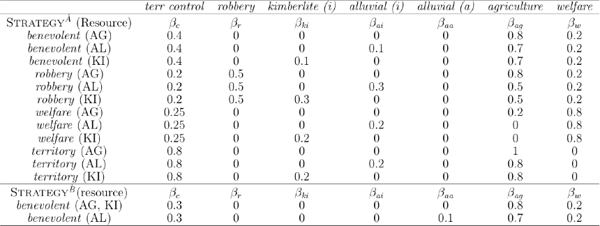
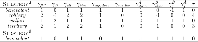
Table A2. Control Strategy Parameters

A.9

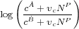
To determine control, we specify a control threshold τ_q > 0, such that if q_c > τ_q, the cell falls under the control of Ȧ, if q_c ≤-τ_q, the cell falls under the control of Ḃ, and for -τ_q < q_c ≤ τ_q, the cell is not controlled by either Ȧ or Ḃ. We define q_c by combing measures of coercive power, peasant sympathy, and geography. Specifically, we use the log ratio of coercive power and and modify this ratio by adding the term υ_cN^P (where N^P is the number of peasants in the cell and υ_C is a constant:

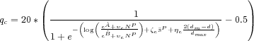
As a result, the cost of shifting control increases with the size of the cell's peasant population. Next, we add ^P to account for the influence of aggregate peasant sympathy on the balance of power in a cell, and η_c to measure the effect of geography (where d is the distance from the cell to the capital city, d_m is the distance to the midpoint between the capital and the border, and d_max is the distance between a border cell and the capital), to obtain:

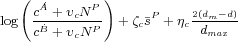
where ζ_c weights the influence of the peasant sympathy and η_c the influence of the geography. The logistic transformation (since we define q_c ∈ [-10, 10]) yields:

Note that conflict in a grid cell makes it impossible for either agent to control this cell.

Notes

¹We gratefully acknowledge comments from Lars Erik Cederman, Chanan Cohen, Nils Petter Gleditsch, Kristian Skrede Gleditsch, Havard Herge, Simon Hug, Eric Little, Ian Lustick, Stathis Kalyvas, Rick Riolo, Nils Weidmann, and participants at seminars organized by the Peace Research Institute Oslo, Center for International Studies at the Swiss Federal Institute of Technology, the University of Michigan's Center for the Study of Complex Systems, the Political Science Department at Michigan State University, and the University of Essex. We also remain indebted to three anonymous reviewers for their comments. Support for this work was provided by the Hebrew University Intramural Research Fund, the Israeli National Science Foundation, and the Department of Political Science at Michigan State University. Additional research assistance with model development was provided by Michael Bommarito II. All faults remain our own.

² A quote from Ross (2006: 265) is instructive: "Studies of natural resource wealth and civil war have been hampered by measurement error, endogeneity, lack of robustness, and uncertainty about causal mechanisms."

³ For a detailed discussion of conflicting results on the resource-civil war relationship, see Ross (2004).

⁴ See Humphreys 2005 for a discussion of plausible mechanisms underlying the resource-civil war relationship.

⁵ For a comparison of exploratory and consolidative modeling see Bankes 2002.

⁶ For a discussion of research strategies using ABM see Lustick and Miodownik (forthcoming).

⁷ The capital city differs from other cells in the landscape given that it serves as a reference point for the government: as the government seeks to control territory further away from the capital city, the cost of control increases monotonically.

⁸ In the description that follows, we use notation consistent with the existence of two ethic groups, with the exception of Demonstration Run I, in which all agents belong to a single ethnic group and where we refer to discontented members (co-ethnics) who seek to overthrow the government as rebels.

⁹ The nature of the resource base has implications for investment and revenue, as well as territorial control. Alluvial diamonds, for instance, are considered "lootable" in that they constitute high value goods with low economic barriers to entry - their extraction by difficult-to-tax artisans requires little in the way of investment and makes it difficult for the state to establish monopoly control over these resources. In contrast, non-lootable resources such as kimberlite or deep-shaft diamonds have high economic barriers to entry - large amounts of capital and technology are required to exploit them profitably, forming a natural barrier that excludes small-scale artisanal miners and makes it easier for the state to establish monopoly control over the resource (by eliminating the need to invest in coercive capacity to deter wildcat miners). Closely tied to the mode of extraction is the location of resource deposits, and we currently distinguish between "point-source" and "diffuse" resource distributions. For more on the resource profiles of alluvial and kimberlite diamonds, their modes of extraction, and implications for civil war, see Snyder and Bhavnani 2005. Note that while we limit our initial focus to agrarian and diamond economies, REsCape may be modified to account for the revenue opportunity structures of other resources such as oil and timber.

¹⁰ Peasant revenue from social welfare y_sw^P is a function of the importance of the cell, and difference between actual and maximal levels of peasant support. We provide additional detail in our discussion of spending strategies in the Appendix.

¹¹ We seek to avoid the possibility of negative ethnic salience, in the event that relative economic well-being is very high. See the Appendix for additional details on our calculation of ethnic salience.

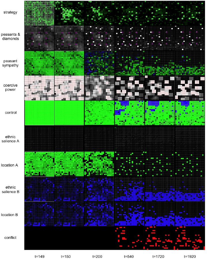
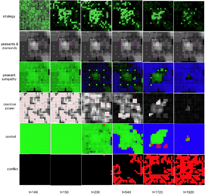
¹² Our selection of snapshots was designed to capture steps during which critical developments occurred.

¹³ Note that our framework restricts rebel investment in industrial mining.

¹⁴ Note that the pockets of the landscape under Ḃ's control in the north of the landscape are a "legacy of the past" in that these are cells that flipped to Ḃ's control but were abandoned shortly thereafter. Given that they remain unpopulated, control never shifts back to the government.

References

AXELROD R (1997) "Advancing the Art of Simulation in the Social Sciences." In Conte, R., Hegselmann, R., and Terna, P. (eds.) Simulating Social Phenomena (Lecture Notes in Economics and Mathematical Systems), Berlin: Springer-Verlag.

AXELROD R and Cohen, M D (2001) Harnessing Complexity: Organizational Implications of a Scientific Frontier, Chicago: The Free Press.

BANKES S C (2002) "Tools and Techniques for Developing Policies for Complex and Uncertain Systems." Proceedings of the National Academy of Sciences of the United States of America, 99, pp. 7263-7266.

BHAVNANI R and Miodownik D (2008a) "Ethnic Polarization, Ethnic Salience, and Civil War." In Progress.

BHAVNANI R and Miodownik D (2008b) "Ethnic Minority Domination and Civil War." In Progress.

BONABEAU E (2002) "Agent-Based Modeling: Methods and Techniques for Simulating Human Systems." Proceedings of the National Academy of Sciences of the United States of America, 99, pp. 7280-7287.

BUHAUG H and Gates S (2002) "The Geography of Civil War." Journal of Peace Research, 39(4), pp. 417-433.

CEDERMAN L-E and Girardin L (2007) "Beyond Fractionalization: Mapping Ethnicity onto Nationalist Insurgencies." American Political Science Review, 101(1), pp. 173-185.

COLLIER P and Hoeffler A (1998). "On Economic Causes of Civil War.'' Oxford Economic Papers, 50(4):563-573.

COLLIER P and Hoeffler A (2004) "Greed and Grievance in Civil War." Oxford Economic Papers, 56(4), pp. 563-595.

COLLIER P and Hoeffler A (2005) "The Political Economy of Secession." In Hannum H and Babbit E F (eds), Negotiating Self-Determination. Lexington Books, Lanham MD.

CONTE R, Hegselmann R, and Terna P (1997) Simulating Social Phenomena. Lecture Notes in Economics and Mathematical Systems. Springer.

DOYLE M W and Sambanis N (2000) "International Peacebuilding: A Theoretical and Quantitative Analysis." American Political Science Review, 94(4), pp. 779-801.

ELBADAWI I and Sambanis N (2002) "How Much War Will We See? Explaining the Prevalence of Civil War." Journal of Conflict Resolution, 46(3), pp. 307-334.

FEARON J D and Laitin D D (2003) "Ethnicity, Insurgency, and Civil War." American Political Science Review, 97(1), pp. 75-90.

FEARON J D, Kasara K, and Laitin D D (2007) "Ethnic Minority Rule and Civil War Onset." American Political Science Review, 101(1), pp. 187-193.

GATES S (2002) "Recruitment and Allegiance: The Microfoundations of Rebellion." Journal of Conflict Resolution, 46, pp. 111-130.

HEGRE H (2002) "Some Social Requisites of a Democratic Civil Peace: Democracy, Development, and Armed Conflict." Paper presented to the Annual Meeting of the American Political Science Association, Boston, MA, 29 August-1 September.

HEGRE H and Sambanis N (2006) "Sensitivity Analysis of the Empirical Literature on Civil War Onset." Journal of Conflict Resolution, 50, pp. 508-535.

HUMPHREYS M (2005) "Natural Resources, Conflict, and Conflict Resolution: Uncovering the Mechanisms". Journal of Conflict Resolution, 49(4), pp.508-537.

LUJALA P, Gleditsch N P, and Gilmore E (2005) "A Diamond Curse?: Civil War and a Lootable Resource." Journal of Conflict Resolution, 49(4), pp. 538-562.

LUSTICK I S, Miodownik D (forthcoming) "Abstractions, Ensembles, and Virtualizations: Simplicity and Complexity in Agent-Based Modeling." Comparative Politics.

MEYER A D, Gaba V, and Colwell K A (2005) "Organizing Far from Equilibrium: Non-Linear Change in Organizational Fields." Organization Science, 16(5), pp. 456-473.

MONTALVO, J G and Reynal-Querol M (2005) "Ethnic Polarization, Potential Conflict, and Civil Wars." The American Economic Review, 95(3), pp. 796-816.

PARUNAK H V D, Savit R, and Riolo R L (1998) "Agent-Based Modeling vs. Equation-Based Modeling: A Case Study and Users' Guide." In Workshop on Multi-Agent Systems and Agent-Based Simulation, Springer, pp. 10-25.

REYNAL-QUEROL M (2002) "Ethnicity, Political Systems, and Civil Wars." Journal of Conflict Resolution, 46(1), pp. 29-54.

ROSS M L (2004) "What Do We Know about Natural Resources and Civil War?" Journal of Peace Research, 41(3), pp. 337-356.

ROSS M (2006) "A Closer Look at Oil, Diamonds, and Civil War." Annual Review of Political Science, 9, pp. 265-300.

SAMBANIS N (2001) "Do Ethnic and Nonethnic Civil Wars Have the Same Causes? A Theoretical and Empirical Inquiry (Part 1)." Journal of Conflict Resolution, 45(3), pp. 259-282.

SNYDER R and Bhavnani R (2005) "Blood, Diamonds, and Taxes: Lootable Wealth and Political Order in Sub-Saharan Africa." Journal of Conflict Resolution, 49(4), pp.563-597.

WIMMER A, Cederman L-E, and Min B (2007) "Ethnic Politics and Violent Conflicts, 1946-2005: A Configurational Approach." Paper presented at the conference Disaggregating the Study of Civil War and Transnational Violence, University of Essex, 24-25 November 2007.

Return to Contents of this issue

© Copyright Journal of Artificial Societies and Social Simulation, [2008]