Diemo Urbig, Jan Lorenz and Heiko Herzberg (2008)
Opinion Dynamics: the Effect of the Number of Peers Met at Once
Journal of Artificial Societies and Social Simulation
vol. 11, no. 2 4
<https://www.jasss.org/11/2/4.html>
For information about citing this article, click here
Received: 29-May-2007 Accepted: 23-Dec-2007 Published: 31-Mar-2008

 Abstract
|
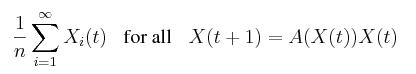
(1) |
|
|
(2) |
|
(3) |
|
(4) |
|
(5) |
|
(6) |
|
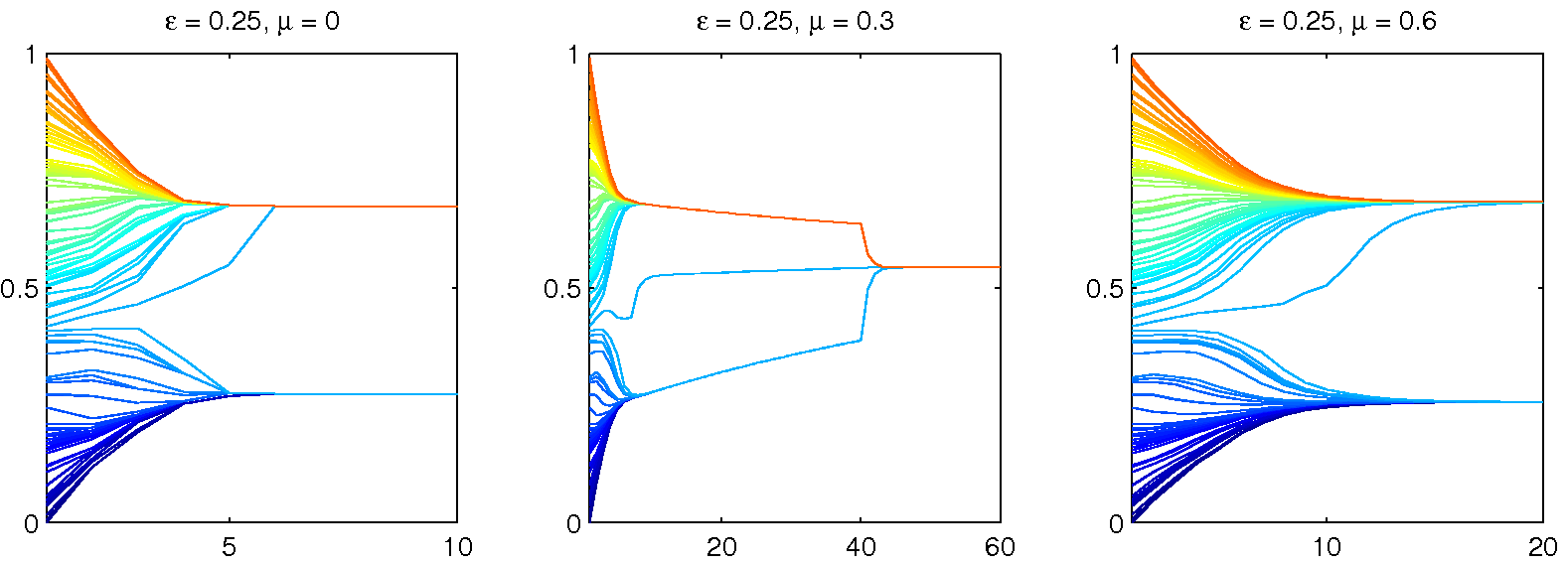
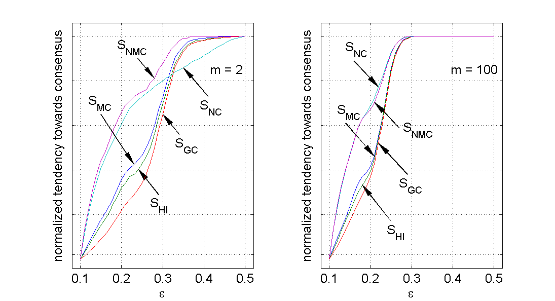
Figure 1. Statistics on the final states for varying ε for m = 2 (left) and m = 100 (right) with n = 100 and μ = 0.0 (click to enlarge the figure)
|
|
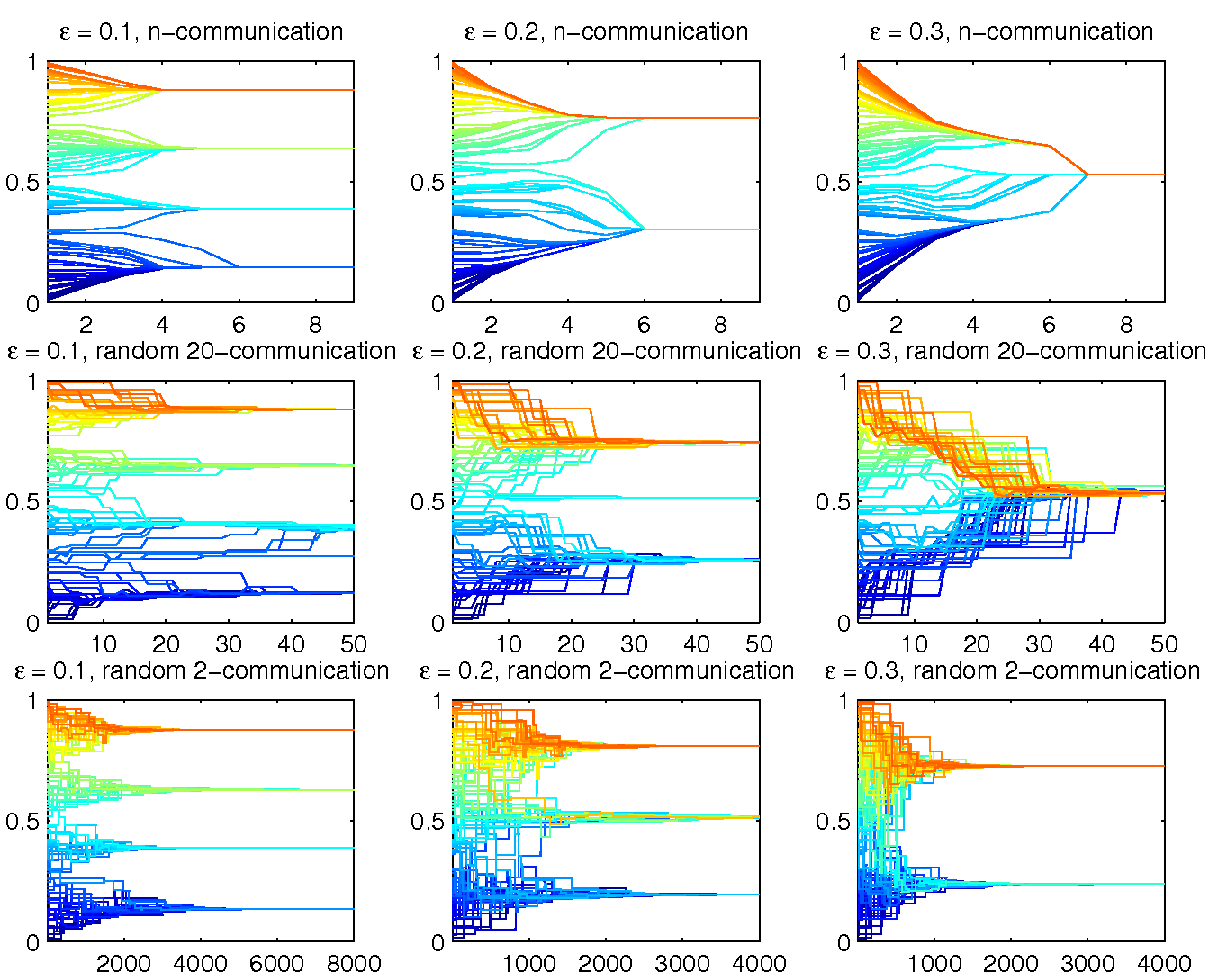
Figure 2. Examples: 100 agents with randomly chosen initial opinions for ε from {0.1, 0.2, 0.3} and for m = n (HK model), m = 20 and m = 2 (DW model) (click to enlarge the figure) |

|
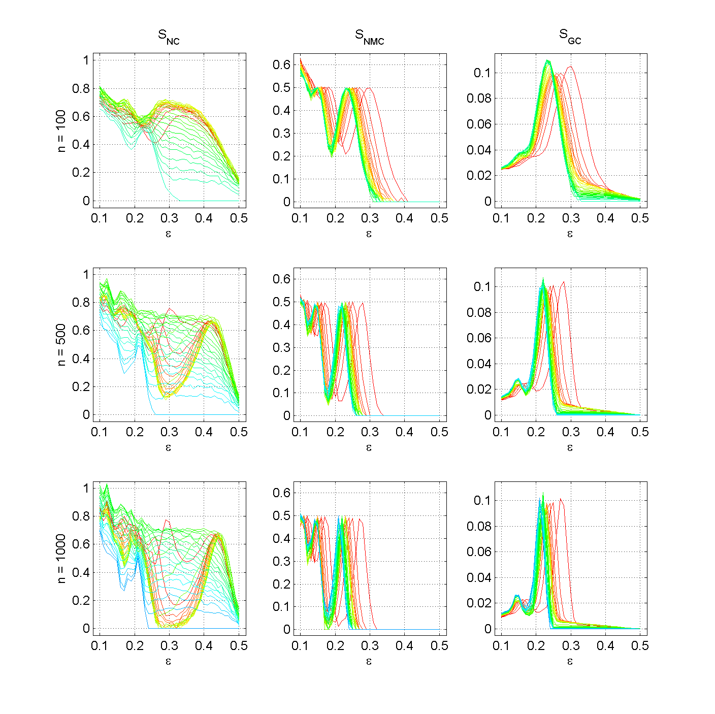
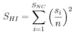
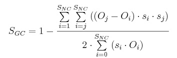
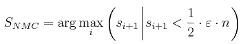
Figure 3. Number of clusters SNC, number of major clusters SNMC, and Gini coefficient SGC for three populations sizes, n ∈ {100, 500, 1000} with μ = 0.0. The lines represent different levels of m (from blue over green and yellow to red, blue represents m = n and red represents m = 2). (click to enlarge the figure)
|

|
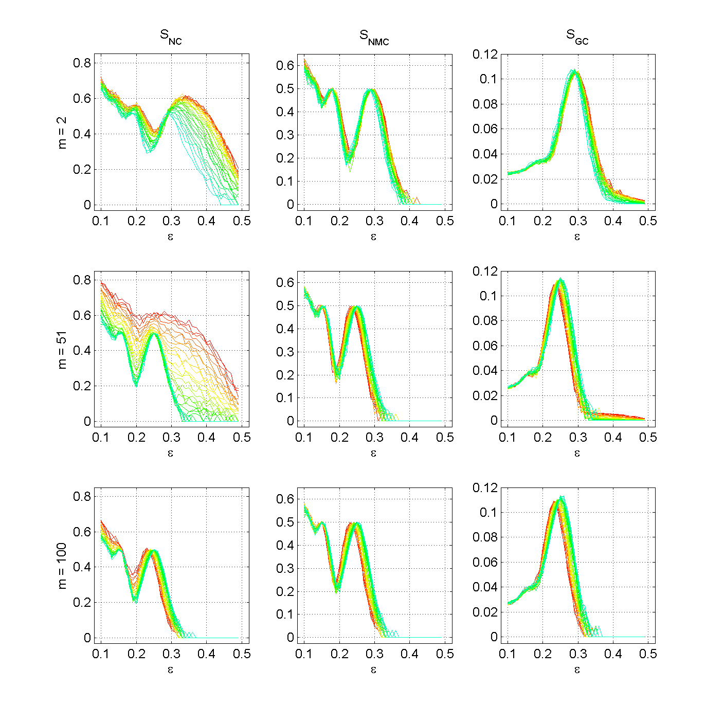
Figure 5. Number of clusters SNC, number of major clusters SNMC, and Gini coefficient SGC for three different numbers of peers met at one m ∈ {2, 51, 100} with n = 100. The lines represent different levels of μ (from blue over green and yellow to red, blue represents μ = 0.9 and red represents μ = 0.0). (click to enlarge the figure)
|
|
Figure 6. Standard deviation of Number of clusters SNC, number of major clusters SNMC, and Gini coefficient SGC for three populations sizes, n ∈ {100, 500, 1000} where the lines represent different levels of m (blue represents m = n and red represents m = 2). This Figure complements Figure 3. (click to enlarge the figure)
|
|
Figure 7. Standard deviation of Number of clusters SNC, number of major clusters SNMC, and Gini coefficient SGC for three different numbers of peers met at one m ∈ {2,51,100} with n = 100. The lines represent different levels of μ (from blue over green and yellow to red, blue represents μ = 0.9 and red represents μ = 0.0). This Figure complements Figure 5. (click to enlarge the figure)
|
|
|
|||||||
| Number of agents n |
Sum of squares |
Sources of variation in proportions of sum of squares | |||||
| WG | BG | ε | m | ε * m | |||
|
|
|||||||
| NC | 100 | 3,151,083 | 0.2340 | 0.7660 | 0.6983 | 0.0535 | 0.0142 |
| 500 | 4,356,244 | 0.1806 | 0.8194 | 0.5993 | 0.1831 | 0.0370 | |
| 1000 | 4,964,100 | 0.1475 | 0.8525 | 0.5785 | 0.2336 | 0.0404 | |
|
|
|||||||
| NMC | 100 | 1,862,348 | 0.1173 | 0.8827 | 0.8673 | 0.0074 | 0.0080 |
| 500 | 1,585,191 | 0.0860 | 0.9140 | 0.8983 | 0.0055 | 0.0102 | |
| 1000 | 1,562,018 | 0.0726 | 0.9274 | 0.9098 | 0.0053 | 0.0124 | |
|
|
|||||||
| GI | 100 | 35,779 | 0.1325 | 0.8675 | 0.8485 | 0.0093 | 0.0097 |
| 500 | 32,460 | 0.0709 | 0.9291 | 0.9040 | 0.0089 | 0.0162 | |
| 1000 | 31,585 | 0.0524 | 0.9476 | 0.9173 | 0.0093 | 0.0211 | |
|
|
|||||||
|
|
||||||||||
| Sum of squares |
Sources of variation in proportions of sum of squares | |||||||||
|
|
||||||||||
| WG | BG | ε | m | μ | ε * m | ε * μ | m * μ | ε * m * μ | ||
|
|
||||||||||
| NC | 3,362,997 | 0.1486 | 0.8514 | 0.7716 | 0.0521 | 0.0034 | 0.0193 | 0.0012 | 0.0029 | 0.0009 |
|
|
||||||||||
| NMC | 2,643,892 | 0.1171 | 0.8829 | 0.8482 | 0.0177 | 0.0001 | 0.0154 | 0.0005 | 0.0005 | 0.0005 |
|
|
||||||||||
| GI | 47.040 | 0.1433 | 0.8567 | 0.8133 | 0.0187 | 0.0001 | 0.0218 | 0.0011 | 0.0008 | 0.0009 |
|
|
||||||||||
2The term 'fully connected' here is not the same as strongly connected in network theory.
3The HK model is not mean-preserving. For instance, with ε = 0.3, μ = 0 and opinion vector (0.2, 0.5, 0.7) one get (0.35, 0.46, 0.6) after one step, which increases the mean from 0.46 to 0.472. Since the HK model is a specific case of our model, also our model is not mean-preserving.
4We have plotted the distribution of cluster sizes and there was a minimum between the peaks of minorities and the peak of majorities that varied approximately as our chosen threshold behaves.
5We are aware that given the previous plots on the standard deviation in different settings, a central assumption of ANOVA, i.e. the homogeneity of variances, is not fulfilled. Nevertheless, the results of the analysis reveal sufficiently huge differences, such that it still sheds some light on the model.
BEN-NAIN, E., KRAPIVSKY, P., VAZQUEZ, F., & REDNER, S. (2003). Unity and discord in opinion dynamics. Physica A, 330, 99–106.
DEFFUANT, G., AMBLARD, F., WEISBRUCH, G., & FAURE, T. (2002). How can extremism prevail? a study on the relative agreement interaction model. Journal of Artificial Societies and Social Simulation 5(4). <https://www.jasss.org/5/4/1.html>
DEFFUANT, G., SKERRATT, S., AMBLARD, F., FERRAND, N., CHATTOE, E., GILBERT, N., & WEISBRUCH, G. (2001). Improving Agri-environmental Policies: a Simulation Approach to the Cognitive Properties of Farmers and Institutions. Final Report, version 2, FAIR3 CT 2092 < http://wwwlisc.clermont.cemagref.fr/ImagesProject/freport.pdf >.
FORTUNATO, S. (2004, march). The Krause-Hegselmann consensus model with discrete opinions. arXiv:cond-mat/0403670v1.
HEGSELMANN, R., & KRAUSE, U. (2002). Opinion dynamics and bounded confidence models: Analysis, and simulation. Journal of Artifical Societies and Social Simulation, 5(3). <https://www.jasss.org/5/3/2.html>
HEGSELMANN, R., & KRAUSE, U. (2004). Opinion Dynamics Driven by Various Ways of Averaging. Computational Economics, 25(4), 381-405.
JAGER, W., & AMBLARD, F. (2004). Uniformity, bipolarization and pluriformity captured as generic stylized behavior with an agent-based simulation model of attitude change. Computational & Mathematical Organization Theory, 10, 295–303.
LORENZ, J. (2005). A stabilization theorem for continuous opinion dynamics. Physica A, 355(1), 217–223.
LORENZ, J. (2007). Repeated Averaging and Bounded Confidence Modeling, Analysis and Simulation of Continuous Opinion Dynamics. Ph.D. thesis at Universität Bremen. (http://nbn-resolving.de/urn:nbn:de:gbv:46-diss000106688)
LORENZ, J., & URBIG, D. (2007). About the power to enforce and prevent consensus by manipulating communication rules. Advances in Complex Systems, 10(2), 251-269.
MASON, W. A., CONREY, F. R., & SMITH, E. R. (2007, August). Situating social influence processes: Dynamic, multidirectional flows of influence within social networks. Personality and Social Psychology Review, 11(3), 279–300.
MOWEN, J. C., & MINOR, M. (1998). Consumer behavior. Prentice-Hall.
SCHWEITZER, F., & HOLYST, J. A. (2000). Modelling collective opinion formation by means of active brownian particles. The European Physical Journal B, 15, 723–732.
STAUFFER, D., SOUSA, A., & SCHULZE, C. (2004). Discretized opinion dynamics of the deffuant model on scale-free networks. Journal of Artificial Socienties and Social Simulation, 7(3).<https://www.jasss.org/7/3/7.html>
URBIG, D. (2003). Attitude dynamics with limited verbalisation capabilities. Journal of Artificial Societies and Social Simulation , 6(1). <https://www.jasss.org/6/1/2.html>
WEISBUCH, G., DEFFUANT, G., AMBLARD, F., & NADAL, J. P. (2001). Interacting agents and continuous opinion dynamics. http://arxiv.org/abs/cond-mat/0111494.
WEISBUCH, G., DEFFUANT, G., AMBLARD, F., & NADAL, J. P. (2002). Meet, discuss, and segregate! Complexity, 7(3).
 Return to Contents of this issue
© Copyright Journal of Artificial Societies and Social Simulation, [2008]