©Copyright JASSS

JASSS logo ----

Marc R.H. Roedenbeck and Barnas Nothnagel (2008)

Rethinking Lock-in and Locking: Adopters Facing Network Effects

Journal of Artificial Societies and Social Simulation vol. 11, no. 1 4
<https://www.jasss.org/11/1/4.html>

For information about citing this article, click here

Received: 25-Apr-2007    Accepted: 08-Nov-2007    Published: 31-Jan-2008

PDF version


* Abstract

When are we locked in a path? This is one of the main questions concerning path dependency. Coming from Arthur's model of increasing returns and technology adoption (Arthur 1989), this paper addresses the question of when and how a lock-in occurs. To gain a better understanding of the path process, different modifications are made. First, the random selection of two types of adopters is substituted with a random selection of adopters having a Gaussian distributed natural inclination. Second, Arthur's model shows only indirect network effects, so direct network effects are added to the model. Furthermore, it is shown that there is an asymptotic lock-in function referring to the technology A and B adopter ratio; this ratio is calculated within the process on the basis of a returning probability to an open state. In the following, the developed model is used to simulate path process without increasing returns, with increasing returns stopping when a lock-in occurs, as well as random drop-outs of increasing returns. One answer that could be drawn out of this new extended model is that there is no lock-in without further stabilizing returns. This and other aspects are used to provide a simplified path-model for empirical research. Finally, its limits are discussed in regard to uncertainty, innovation, and changes in network effect parameters.

Keywords:
Path Dependence, Gaussian Distributed Adopters, Network Effects, Dynamic Information Distribution, Lock-in Calculation

* Introduction

1.1
Path dependence is a rather old concept in economics (for example Arthur et al. 1983; Arthur 1988, 1989). It was developed out of a mathematical discussion of network effects influencing market processes based on a model of adopters choosing among two or more technologies. Arthur (1989) showed that, under the condition of a random selection of adopters, each having a natural inclination towards one of the two alternatives plus the weighted network effects, the sequence of their appearance at the market influences the non-ergodic outcome. Those effects lead to the dominance of one alternative which is comprehensible from a neoclassical point of view, as long as the evolved market solution is the best alternative. But Arthur showed that, due to the timing effects, the ’best’ or most efficient solution does not necessarily win the competition. The network effects lead from initial multiple possible equilibriums to potentially inefficient lock-ins, which was formulated as the major characteristic of path dependent processes (Arthur et al. 1983; David 1985; Arthur 1988, 1989, 1996). Focussing on other aspects, Arthur unfortunately did not analyze the point or phase of lock-in in detail. He argued that the result in some cases is somehow locked.
1.2
Different understandings in the assumptions of path dependence and its challenge to neoclassical economics have led to an intensive debate ( Liebowitz & Margolis 1990, 1995, 2001). Liebowitz and Margolis state that there is only one "form of path dependence that conflicts with the neoclassical model of relentlessly rational behaviour leading to efficient, and therefore predictable, outcomes" (Liebowitz & Margolis 1995: 207). This form is characterized by an action carried out, although the adopters know that it leads to an inferior outcome. They therefore postulate that path dependence is based on unrealistic and respectively improbable assumptions. However, this criticism is supporting the neoclassical efficient equilibrium paradigm targeted by path dependence. This paradigm is founded on the assumption of rational actors, aggregating their individual rationalities to a collective rationality: if profit opportunities are available, there will be an entrepreneur breaking the path. If there is no such opportunity, the prevalent solution is the best, even when it is technologically inferior (Liebowitz & Margolis 1995: 314ff.). These criticisms reveal some theoretical issues of path dependence worth discussing, but do not refute the general applicability (Ackermann 2001). In contrast to the criticisms, the concept of path dependence considers the interdependencies between multiple actors, their natural inclinations and actions, leading to a single but not obligatory collective rational behaviour.
1.3
Taking the concept of path dependence as a possible model for explaining lock-ins in markets or organizations, scholars from organization science have raised a central question in their research [1]: How can path dependence be detected and its rigidity eventually be quantified? This is of major interest, considering the power of hyperstable equilibriums. What amount of resources, knowledge, technologies, manpower or time have to be spent to overcome these rigidities? In the case of inefficient outcomes, this may be a question of survival for an organization; in a broader sense, this may be a question of inertia and the unchangeability of markets. For example, politics may suffer from such equilibriums impeding public reforms and change.
1.4
Some empirical examples for markets and organizations can be found that try to transfer some or all of the three theoretical main characteristics of paths: 1) multiple equilibriums, 2) increasing returns, and 3) lock-in on a potentially inefficient path (see, for example, Britton 2004; Bruggemann 2002; Puffert 2002; Cowan & Gunby 1996; Helfat 1994). But these authors do not explain what kind of increasing returns influence the process and how a lock-in may result. In more recent literature by scholars from organization science, for example, these three characteristics are mapped onto three different phases (Sydow et al. 2005; Schreygg et al. 2003). After a phase of random selectivity, a phase of increasing returns follows, that finally switches into the lock-in. Obviously, this corresponds with Arthur’s stages of small events, positive feedback, and lock-in. The increasing returns in this model are modified to organizational self-reinforcing mechanisms or positive feedback loops; the networks effects described by Arthur are included as resource-based positive feedback effects. But, due to the many perspectives on this issue of self-reinforcement, it has been hard to identify a general canon of self-reinforcing mechanisms; especially how they operate and how they may be measured (compare Beyer 2005 vs. Sterman 2000 vs. Sydow et al. 2005 for attempts to systematise the mechanisms).
1.5
But before the attempts to transfer Arthur’s concept of path and the underlying assumptions to a less technological field like social systems, some questions should be answered. First, theoretical basics can be addressed by the following set of questions: What happens to a simulated path process if the adopters can not be separated into two groups? Why are only indirect network effects in action? What happens to the early random phase in Arthur’s model when adding network effects? What happens to Arthur’s model when the fixed variables are chosen differently? When does a lock-in occur in the path process, and how can it be measured? And with a second set of questions, the transfer to empirical social science can be addressed: What happens to path processes if no increasing returns are present? What happens to path processes when the increasing returns randomly stop within the process? What happens to path processes when the increasing returns stop after the lock-in? What issues need to be shown in empirical research to prove the model of a path explaining lock-in?
1.6
In order to answer the first set of questions and provide insights for developing a better understanding of and suggestions for the measurement of increasing returns as well as a resulting lock-in, this paper[2] starts with a theoretical discussion and extension of Arthur’s model. This is the precondition for transferring the concept of path into empirical social science and answering the second set of questions.
First, the mode of selection for each adopter is changed. Therefore the 50/50 random choice between two types of adopters is replaced with the selection of one adopter with a randomly selected Gaussian distributed natural inclination. This means that most adopters tend only slightly to one alternative. With competing technologies (as substitutes) this is a more realistic scenario. Second, direct network effects are added to the indirect network effects in Arthur’s model, simulating the additional utility of total sharing possibilities in a network. Different technologies and markets may have different network effects with different intensities. Third, the weighting of both network effects is simulated by two logistic functions, representing the information diffusion from the network of past adopters to the new ones. As in the second point, the intensity of both network effects may vary over time differently, so they should not be equated with a fixed value as in Arthur’s model. Fourth, Arthur’s assumption of the lock-in as the point where the utility of every adopter is determined by the network effects is replaced. The network effects are present at the market throughout the entire time of the process and so the lock-in needs to be calculated. Therefore the probability of returning to an open state of the process is used; this is marked, ceteris paribus, by an equal number of adopters for every technology.
Regarding the discussion, the second set of questions is addressed using the extended model. The increasing returns are switched of at various points so that implications for future research can be provided.

* Arthur’s Model of Path Dependence

2.1
To give an introduction to the common understanding of a path dependent process, the model developed by Arthur and his colleagues (1983, 1989) is shown in a short step-by-step version. At first the random walk process is shown and the modification to a random walk with a lock-in barrier. Then, the non-linear probability case of the Polya urn was used to develop the final model of two randomly selected adopters with specialized natural inclinations under increasing returns.

Random Walk Processes

2.2
The basic model of path dependence was developed by Arthur and his colleagues (1983, 1989), who extended the Polya urn process by non-linear dynamic probabilities dependent on the market share or the total number of technology adopters. This was a theoretical modelling of the QWERTY case analysed some years earlier (David 1985). In his 1989 paper Arthur starts with a description of a market as a simple random walk process; two types of adopters (R-adopters prefer technology A and S-adopters prefer technology B) choose between the two alternative technologies A and B. Both technologies have a fixed probability of selection of 0.5 by each adopter at every step. This probability can not be influenced by sponsoring or advertisements or any other external force. In this case, the observer of the market is not able to predict the final outcome; it seems that all adopters choose randomly.
2.3
This can be simulated using two stacks A and B, where the number of selections for each technology is counted. For a selected number of adopters, a process creates a uniformly distributed random number within the interval of 0 and 1, and then selects which stack is to be increased according to the fixed probability. At each step, the difference between both stacks (simple subtraction) and the market share distribution (ratio of one stack in comparison to the sum of both stacks) is plotted. The pseudo code for simulating [3] this random walk is shown in Code 1:

//Initializing the Stacks
stack_a = 1;
stack_b = 1;

//Run the loop for a given number of adopters
for (x = 0 to (adopter-1)) {
//uniformly distributed random number
random = (rand(0,1000) / 1000);

//decide according to fixed probability of 0.5
if (random < 0.5) {
stack_b ++;
} else {
stack_a ++;
}

//graphical output
draw_adopter_difference (x, stack_a - stack_b);
draw_market_ratio (x, stack_b / (stack_a + stack_b));
}
Code 1. Random walk
This pseudo code represents a snippet from the full program only (lines 339-435); a complete
version (with PHP/Winbinder) may be downloaded from here and run under Windows

2.4
Running this random walk process with an outer loop of simulations 20 times (grey lines) with an inner loop of 500 adopters (abscissa), each choosing one technology, the result of the difference between the number of adopters for alternative A and B (ordinate) is alternating around zero (see Figure 1):

Figure
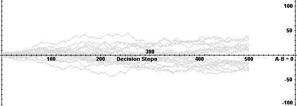
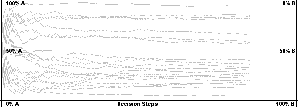
Figure 1. Adopter difference of random walk

2.5
Having a closer look at the market share distributions of alternative A and B (left ordinate for A and right ordinate for B), the results for this 20-time random walk (grey lines) alternates around 50 percent for both (see Figure 2):

Figure
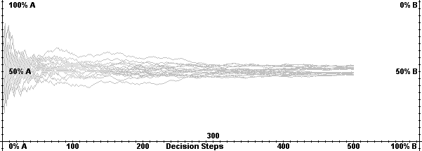
Figure 2. Market share distribution of random walk

Random Walk Process with a Lock-In Barrier

2.6
In a second step, Arthur shows the impact of history, depending on the number and sequence of previous adopters, by defining a random walk process with an absorbing barrier. This barrier represents a certain difference between adopters of technology A and B. Crossing this barrier means locking the process (Arthur et al. 1983, 1985; Arthur 1989). From then on, both types of adopters choose, independently from their initial preference, the dominating technology (Arthur 1989: 120). The pseudo code in PHP from above only needs slight modifications by introducing an if-routine that checks whether this fixed rate barrier is reached. From then on, the random number is set to a fixed value needed for following the dominant design (see Code 2):

//Initializing the Stacks
stack_a = 1;
stack_b = 1;

//Run the loop for a given number of adopters
for (x = 0 to (adopter-1)) {
//uniformly distributed random number
random = (rand(0,1000) / 1000);

//check if barrier has been crossed
if ( [checkbox ’barrier’ is TRUE] ) {
//test if A-B is bigger than barrier
if (stack_a - stack_b >= barrier ) {
random = 1;
}
//test if B-A is bigger than barrier
if (stack_b - stack_a >= barrier ) {
random = 0;
}
}

//decide according to fixed probability of 0.5
if (random < 0.5) {
stack_b ++;
} else {
stack_a ++;
}

//graphical output
draw_adopter_difference (x, stack_a - stack_b);
draw_market_ratio (x, stack_b / (stack_a + stack_b));
}
Code 2. Random walk with absorbing barrier
This pseudo code represents a snippet from the full program only (lines 339-435); a complete
version (with PHP/Winbinder) may be downloaded from here and run under Windows

2.7
The result of this modified random walk process alternates around 0, again using 20 simulations and 500 adopters each (grey lines). But as soon as the absorbing barrier of technology dominance (in this case 30 adoptions) is passed, the process turns into a linear function, with a slope of 1 (see Figure 3). The linearity is caused through the direct impact of the adopters’ selection on the difference between the number of adopters for alternative A and B. Each new adopter for the locked alternative (ones A and two times B in Figure 3) increases the difference in each step by 1:

Figure
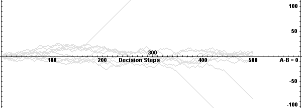
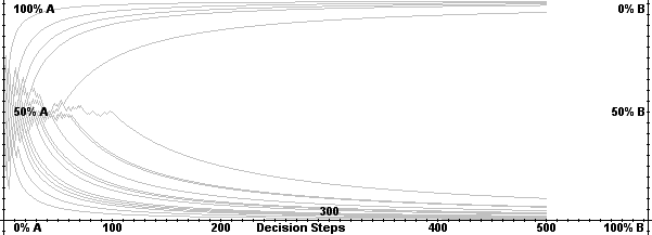
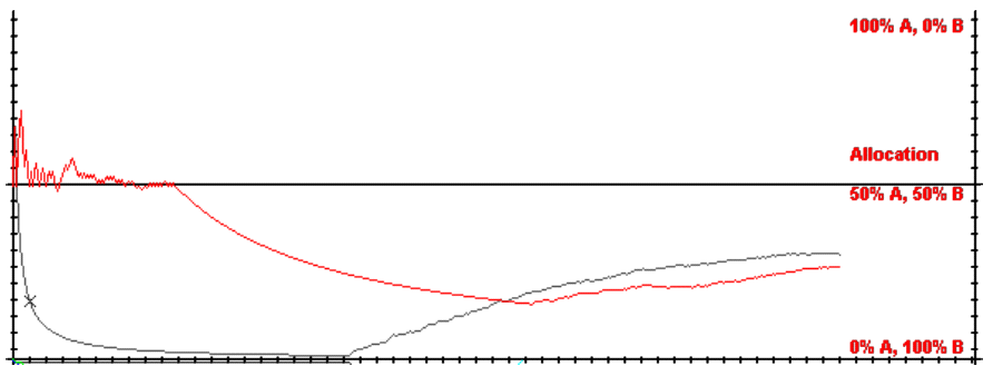
Figure 3. Adopter difference of random walk with absorbing barrier

2.8
Of course, the linearity of the difference between the number of adopters for alternative A and B after the absorbing barrier of 30 adoptions is not reproduced in the case of market share distribution. The distribution of market shares looks like a ’normal’ random process in the beginning (compare to Figure 2), and turns into an asymptotic function after the barrier is crossed (see marks in Figure 4). This is caused by the softer impact of the locked alternative on the ratio (especially the denominator). The longer the process runs, the bigger the stack of both alternatives is and the smaller the impact is of each new selection. With an infinite number of adopters, the market share distribution would finally result in 99 percent (in this case, once for technology A and twice for technology B):

Figure
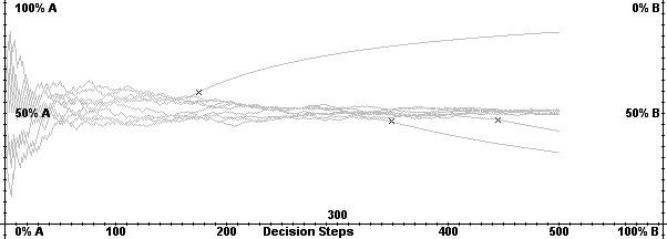
Figure 4. Market share distribution of random walk with absorbing barrier

Polya Urn Process

2.9
Regarding the impact of previous drawings, and to overcome the arbitrarily selected barrier, Arthur uses the Polya urn example, seen only as a soft version of an increasing return process in recent economic path dependence literature (Sterman 2000). The Polya urn is filled initially with two balls of two different colours. A ball is drawn randomly and put back into the urn with one additional ball of the same colour (Arthur 1994: 6). By using this model instead of a normal random walk process, the development of market shares can be simulated more realistically, because the result does not always tend to a fifty-fifty distribution and is no longer predictable. The potential inefficiency of this outcome is obvious, not only for technological adaptation but also for institutional adaptation (Caldas & Coelho 1999).
2.10
The pseudo code in PHP from the simple random walk (see Code 1) now again needs a few modifications: For each simulation, the inital stacks are set. Then, in each round of the adoption process, at first a uniformly distributed random number between 0 and 1 is generated. As a second step, the present market share distribution is calculated as the ratio of one stack compared to the sum of both stacks. Due to the balls inside the Polya urn, this ratio is compared to the uniformly distributed random number [4] and one of the two alternative stacks is incremented by one (see Code 3):

//Initializing the Stacks
stack_a = 1;
stack_b = 1;

//Run the loop for a given number of adopters
for (x = 0 to (adopter-1)) {
//uniformly distributed random number
random = (rand(0,1000) / 1000);

//calculate market share ratio
ratio = stack_b / (stack_a + stack_b);

//decide according to fixed probability of 0.5
if (random < ratio) {
stack_b ++;
} else {
stack_a ++;
}

//graphical output
draw_market_ratio (x, stack_b / (stack_a + stack_b));
}
Code 3. Polya urn process
This pseudo code represents a snippet from the full program only (lines 438-501); a complete
version (with PHP/Winbinder) may be downloaded from here and run under Windows

2.11
Interestingly, the distribution of market shares in the case of the Polya urn is completely different from the distribution of market shares in the case of a random walk crossing fixed barriers (compare Figure 4). The decision of the adopters in the case of the Polya urn is not a random process with a fixed probability of 50 percent for each technology. The adopters now decide according to the market shares already present. As a result, the alternative which is represented with a higher market share in the early steps is selected more often afterwards. Losing the quality of predictability in the beginning (as stated above), every allocation ratio between the two alternatives is possible (see Figure 5). But after some initial steps have passed, the final market share distribution can be closely predicted - a first mover advantage:

Figure
Figure 5. Market share distribution of the Polya urn process

2.12
In this soft ’history matters’[5] process, past actions influence the outcome, because the addition of another ball into the urn represents a reproduction with a constant factor (Liebowitz & Margolis 1995). The issue of inefficiency is not considered here.

Adopters with Specialized Natural Inclinations and Increasing Returns

2.13
The increasing return process, which goes beyond this soft ’history matters’ argument of the Polya urn, requires further modifications. Arthur (1988, 1989) argues that the decision of the actors (R and S) needs to be redirected on their return for each technology (A or B), depending on their natural inclination for one alternative (aR or bR with aR > bR; aS or bS with aS < bS ) plus the weighted (r, s) number of past adopters (the stack of A or B) for the technology (see Table 1).

Technology ATechnology B
R-agentaR + rnAbR + rnB
S-agentaS + snAbS + snB
Table 1. Arthurian agents with network effects

2.14
He considers the weighted number of past adopters as a network effect that is integrated into the decision of the adopters at a certain point in time. The random decisions are replaced by network dependent decisions but with a random appearance of different types of adopters at the market. So the uniformly distributed random number is needed to determine whether an adopter of type R or S is the next to choose under market conditions. Then their utility is calculated dependent on the weighted stack and their natural inclination. Regarding past simulation studies (for example Leydesdorff & Besselaar 1998: 311), Arthur’s process can be pseudo-coded in the following way (see Code 4):

//Initializing the Stacks
stack_a = 1;
stack_b = 1;

//Run the loop for a given number of adopters
for (x = 0 to (adopter-1)) {
//uniformly distributed random number
random = (rand(0,1000) / 1000);

//calculate the utility of an adopter according to which one is selected
if (random < 0.5) {
return_a = ar + (r * stack_a);
return_b = br + (r * stack_b);
}
if (random >= 0.5) {
return_a = as + (s * stack_a);
return_b = bs + (s * stack_b);
}

//check whether the utility for A or B is higher for present adopter
if (return_a > return_b) {
stack_a ++;
} else {
stack_b ++;
}

//graphical output
draw_market_ratio (x, stack_b / (stack_a + stack_b));
}
Code 4. Arthur’s simple model
This pseudo code represents a snippet from the full program only (lines 503-630); a complete
version (with PHP/Winbinder) may be downloaded from here and run under Windows

2.15
By choosing values for the constants introduced in Arthur’s model (according to Leydesdorff & Besselaar 1998: 311), the market share distribution of both technologies looks like a random walk process in the beginning (easily observable from the grey line in the middle with the longest random phase; see Figure 6), but shifts into a steeper asymptotic function than in the case of a random walk with an absorbing barrier (compare to Figure 4). This is mainly caused by the increasing returns which dominate the decision process after the phase of the adopters inclination as the main decision criteria:

Figure
Figure 6. Market share distribution of Arthur’s urn process

* Limits of Arthur’s Simple Model and his Advanced Extensions

3.1
Arthur’s original model is a robust one, even under its restrictions and assumptions. Many of his assumptions are applied for simplicity reasons and do not change the basic results of the model if altered. Some of them can be accepted as having little influence on the outcome. These are changes in the number of adopter types, changes in the number of technologies, an unequal number of adopters for both technologies in the beginning, and competing technologies that do not start at the same time. In the case of N competing technologies, the model is easily extended to N dimensions. But due to the unchanged mechanisms of technology adoption, the results remain the same, as shown in the Arthur-Emoliev theorem (Arthur 1989). Another assumption was the lack of sponsoring regarding the technologies. But it can also be easily integrated into Arthur’s model, and it only shifts the absorbing barriers closer towards the fifty-percent straight line (see Figure 3). This represents an earlier lock-in, because the utility of each adopter is supported in favor of the sponsored technology. Regarding the possibility of an unequal proportion of R and S adopters in the beginning of the process, there are also no major influences on the model. The simple random walk would drift (similar to the case of sponsoring) towards the technology with the higher proportion of adopters: The probability of meeting the associated absorbing barrier is higher than before. Last but not least, a similar scenario is that competing technologies do not start at the same time. This means that only one technology is adopted before the other enters the market. A higher proportion for the leading technology in the beginning of the process results in a first mover advantage, leading to a higher probability of being the dominant technology in the end (Arthur 1994: 24). All these examples show variations which do not influence the process.
3.2
But altering other basic assumptions of Arthur’s model will have a deeper impact on the process and its possible results. Some of the simplifications due to the basic assumptions of Arthur’s modelling were already addressed in the first set of introductory questions. First, there are only two kinds of adopters present (Arthur 1989: 117) where the selection between them is based on a uniformly distributed random number; a random walk of R and S adopters emerges. Even in Arthur’s extension to a continuum of adopter types with a vector of natural preferences reagarding the technologies on the market (Arthur 1989: 125), those inclinations are arbitrarily set. Therefore the simulation of a set of adopters with normal distributed prefernces over a bipolar continuum reflects the empirical findings (especially when talking about large numbers) when looking at preferences for new and competing technologies. Also, the effects of the dynamic probability of technology adoption within the selection process (like in the Polya urn case) are not considered (Leydesdorff & Besselaar 1998). So it is more plausible using one type of adopter with infinite types of possible natural inclinations or preferences that follow a special kind of distribution function.
3.3
Second, Arthur uses only one type of network effect that can only take place if the actors are reflexive (Garud & Karne 2001), i.e. they look at the market and previous decisions and recognize the benefits resulting from the network. This theoretical thought is implicitly integrated within the simple model. Making it explicit, the reflexivity of actors results in two different types of network effects. Indirect network effects, as used in Arthur’s model, represent the utility of past adopters choosing the same technology. Each adopter does not need to have contact with other adopters: the increase of DVD rental stations is a result of sales rates. Direct network effects represent the additional utility of total sharing possibilities in a network, i.e. the total number of possible links in a network. Each adopter needs to stay in contact with others and benefits also from their connections when sharing DVDs. So both types of network effects should be taken into account when simulating path processes based on network effects.
3.4
Third, the arbitrarily selected and fixed values for the constants of network effect coefficients in Arthur’s model, as done in simulation studies (Leydesdorff & Besselaar 1998), are problematic. The dynamics of network effects according to their relative increasing and decreasing impact on technology distribution can not be shown with constants. Dynamic coefficients, for example derived from the increasing speed of information distribution and information thickness in growing networks (information diffusion), are needed to reflect this (Dodson & Muller 1978). Now it is possible to weigh the different network effects at different points in time, leading to a more flexible simulation.
3.5
Fourth, Arthur assumes that markets expand infinitely, or at least as long as a lock-in can happen. Although Arthur’s urn is seen as a member of the innovation distribution research, it does not integrate the market limits (compare to Bass 1969; Sahal 1981; Rogers 1983; Strobel & Roedenbeck 2006). Therefore, it is necessary to limit the number of adopters in the model depending on the analysed market. Of course, these can be large numbers (Leydesdorff 2000), but in this study, a screen resolution of 500 pixels is used so that each pixel represents a decision. The results can therefore be better analysed compared to interpolated simulation studies. But on the other hand, only a few markets have such a small number of customers. Regarding past simulation studies, the main influences of increasing returns can be observed in the beginning of processes, which also supports a small number of adopters (n=500). The market limit also has an effect on the information diffusion concerning the network effects; in a smaller market, the influence of network effects may have a steeper and faster impact than in larger markets. With this modification it can also be tested if a market is large enough to lock in.
3.6
Fifth, there are two aspects to discuss regarding the barriers in Arthur’s model . One is that he equates the barriers in the first step of his model (Arthur 1989) with a fixed difference in the absolute numbers of adopters for each technology. This may be practical, but is not persuasive, because at a later point in time, this difference appears more easily without any reason. Additionally, the value of the barrier to break is arbitrarily set. In his second model (Arthur 1988, 1989), he uses the term lock-in to describe the point in time where all adopters switch to the dominant alternative because of the strength of network effects representing the higher utility for every adopter. This is a structural lock-in (Leydesdorff & Besselaar 1998: 310). But because in reality all adopters are able to choose at any point in time what they prefer, it is possible that even after the lock-in occurs the non-dominant technology is selected. When these adopters appear at the market in a sequence, the 'locked' market might be turned into a non-locked one again. So it would be more persuasive to define the lock-in as a point in time when the probability of returning to an equal proportion of adopters for both technologies decreases below a specific value. The second aspect is that, in Arthur’s model, the increasing returns do not cause any effect on the decision of the adopters unless one of the network effects exceeds the difference of the natural inclinations (Arthur 1989). This results in a random walk until all adopters switch to the dominant design. Hence, there would be no difference between the point where increasing returns start to influence the decision and the occurrence of a lock-in. Obviously, increasing returns influence the decision process before and after the lock-in. Even one adopter can lead to network effects in reality and the model should reflect the effects in the decision rules of the adopters right from the beginning.

* Modification of Arthur’s Urn Model

4.1
The problems discussed above can be handled by modifying Arthur’s extended model. Step by step, Arthur’s table (1989) is redesigned to support those arguments. This is done in four steps: 1) the two adopters and their natural inclinations are reduced to a single normal distributed function (Gaussian distribution) for reflexive actors; 2) the direct network effects are added to the indirect ones; 3) the weighting of both network effects is simulated by two logistic functions; and 4) the lock-in calculation is based on the possibility of returning to an equal distribution of adopters.

The Gaussian Distributed Function as Adopters ’Natural’ Inclinations

4.2
The two adopters in Arthur’s model each have a different natural inclination towards both technologies. At first, this assumption seems to be reasonable. Perhaps local settings or bi-characteristic attributes (male/female, etc.) are responsible for this inclination. However, competing technologies are seen as substitutes. In the simple model, the adopters are divided by those two competing technologies into two distinct separate and homogenous groups regarding their fixed natural inclinations. Arthur’s extension uses a continuum of adopters with fixed arbitrary set preferences across two or multiple technologies (see Figure 7, left), but he does not apply a function for the underlying selection process. This can lead to a systematic bias due to the random selection of adopters. It makes little sense regarding ’competing technologies’.
4.3
Of course, technologies adopted due to these characteristics will not be abandoned if a lock-in occurs. From the economic demand curve for substitutes (here: competing technologies), we derive adopters’ inclinations distributed over the whole spectrum of possible inclination combinations (see Figure 7, right). For simplicity reasons, we use the Gaussian distribution representing all adopters and their natural inclinations:

Figure
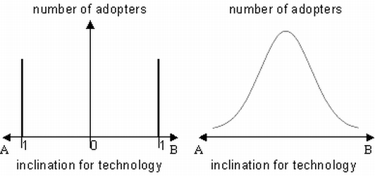
Figure 7. Frequency distribution of Arthur (1989) and the new model

4.4
Realistically, most adopters seem to have no difference or at most small differences in their natural inclination. This is represented by the peak at the median of the Gaussian adopter function. Now, the adopters have a randomly chosen inclination towards one technology (let’s say a), and the effect on the technology decision depends on the position in the Gaussian function. Hence the inclination for the other technology B is the negated value (1-a). Other functions, such as a uniform distribution or a function with a u-shaped curve, may be good alternatives as well, depending on the product observed. But they have to be confirmed empirically. Nevertheless, these continuously differentiable spectrums of adopters allow a more realistic perspective on the adoption processes. Arthur’s table (compare to Table 1) with Gaussian distributed adopters and weighted network effects now looks like the following (see Table 2):

Technology ATechnology B
G-agenta + rnA(1-a) + rnB
Table 2. Gaussian distributed actors for two technologies

4.5
Producing a Gaussian distributed random number is more difficult in PHP, because there is only a random number generator for uniformly distributions. Using the Box-Muller method (Box & Muller 1958), the Gaussian distribution can be derived out of two uniformly distributed random numbers. Both random numbers are multiplicated after they have been transformed using a logarithmic function with the base 10 for the first and a sinus function for the second number. Regarding Arthur, who sets the initial preferences between 0 and 1, the Gaussian distribution needs to be modified with its mean of 0 and a variance of 1. It is moved from the mean of 0 to a mean of 3, because only 0.27% of the drawings are above or below a triple of the variance, which is one in the Gaussian distribution. Then the moved distribution is compressed to a distribution between 0 and 1 by dividing the result by 6; this is twice the triple of the variance (see Code 5):

function gauss() {
//make two uniformly distributed random numbers betwen 0 and 1
random1 = (rand(0,1000) / 1000);
random2 = (rand(0,1000) / 1000);

//calculate the random number in a Gaussian distribution using Box & Muller
//log in php = ln
gauss = squareroot ((-2) * log(random1)) * sin(2 * pi * random2);

//correction of the random number to a distribution between 0 and 1
gauss_modified = (gauss + 3)/6;

return gauss_modified;
}
Code 5. Reflexive Gaussian distributed actor
This pseudo code represents a snippet from the full program only (lines 128-135); a complete
version (with PHP/Winbinder) may be downloaded from here and run under Windows

The Application of Indirect and Direct Network Effects

4.6
Arthur adds the network effects to the payoff utility for every adopter represented by the ’natural’ inclination (see Table 1). This second term of network effects increases constantly with the number of adopters. Therefore every adopter benefits from the increasing number of adopters of his technology. This indirect network effect (INE) can easily be integrated into the pseudo code using the present stack of adopters with Arthur’s weighting (see Code 7):

//weighted indirect network effects for A
INE_a = stack_a * r_a;
//weighted indirect network effects for B
INE_b = stack_b * r_b;
Code 7. Indirect network effects
This pseudo code represents a snippet from the full program only (lines 693-695); a complete
version (with PHP/Winbinder) may be downloaded from here and run under Windows

4.7
But indirect network effects (INE) do not work alone in network markets. Direct network effects (DNE) are also present, which are different from the indirect ones and must be integrasted into the model. With the rise of telecommunication, people buying a telephone attained their utility not from being part of a community having a telephone, but from using it. This resulted in a direct network effect (DNE) with the possibility to connect to others: ’n-1’. But the additional utility of all connection possibilities in a network is larger, because the adopters can benefit from their connections as well as from the connections used by others. So the direct network effect (DNE) can outstrip the indirect network effect (INE). Focusing on this aspect, Kemp uses a sinus term as an alternative for the network effects (Kemp 1999). This may be useful for the analysis of paths concerning consumers and commodities, but it is not applicable in the case of steadily growing network effects. The new meaning of the utility function implies indirect network effects and direct network effects and moves closer to the interdependence of the adopters and their growing utility with a growing number of technology adopters. Reflexivity, market observation, and the knowledge of the number of previous adopters for every technology by every adopter are assumed. Applying those interpretations to the decision function without any attenuation or weighing would cause an unrealistic impact. The modification of Arthur’s table with both (INEA, INE B for indirect and DNE A, DNE B for direct) weighted (r) network effects looks like the following (Table 3):

Technology A Technology B
G-agenta + INEA(r) + DNEA(r)(1-a) + INEB(r) + DNEB(r)
Table 3. Gaussian distributed actors for two technologies
with direct and indirect network effects

4.8
Focusing on the calculation of the direct network effect (DNE) all connection possibilities in a network need to be recognized. This can be simulated by the number of all possible connections between all participating adopters. Mathematically, this assumption can be expressed using the formula for triangular numbers, which is written as follows:

c(n) = n (n-1) / 2(1)

4.9
The triangular function for direct network effects (DNE) can be provided with the following PHP pseudo code (see Code 8):

//weighted direct network effects for A
DNE_a = (stack_a * (stack_a-1) * (1/2)) * r_a;
//weighted indirect network effects for B
DNE_b = (stack_b * (stack_b-1) * (1/2)) * r_b;
Code 8. Direct network effects
This pseudo code represents a snippet from the full program only (lines 697-699); a complete
version (with PHP/Winbinder) may be downloaded from here and run under Windows

4.10
Different to the decision rule described by Arthur, where the increasing returns have no effect as long as the natural inclination is higher, the natural inclination and each network effect are summed up for both technologies. By this, the network effects can take place right from the beginning of the process. The difference of those utility functions is then used to determine which technology provides a higher return. The PHP code looks like the following (see Code 9):

//calculate the utility difference for one adopter for both technologies
utility_diff = (a + INE_a + DNE_a) - ((a-1) + INE_b + DNE_b);

//add decision for technology depending on the bigger utility
if (utility_diff < 0) {
stack_b ++;
}
if (utility_diff > 0) {
stack_a ++;
}
Code 9. Decision rule depending on difference between utilitys
This pseudo code represents a snippet from the full program only (lines 701-714); a complete
version (with PHP/Winbinder) may be downloaded from here and run under Windows

4.11
This decision rule shows that the coefficients of direct and indirect network effects can have a large impact on the outcomes. Holding them constant facilitates analyses but blurs other effects as well. They are therefore modified in the next step.

The Application of Dynamic Coefficients

4.12
Weighing the indirect and direct network effect is important, according to Arthur (1989), because the unweighed stack of technologies would have a large and deep influence on the behavior of the market share distribution. To solve this problem, Arthur (1989) selects a fixed value for technology A and B (r and s). But it is not taken into account that a small distribution of one product has a low impact on present adopters when selecting a fixed value, because the adopters might not be members of a network (direct network effects), for example, or they might be so few that companies do not provide great support (indirect network effects). With a larger distribution of technology, the influence on direct and indirect network effects rises. The future adopters recognize effects and utilities of previous adopters and estimate their utility for every possible alternative. So the factors for the decision rules alter for some adopters. Drawing the conclusion that a large distribution has also a high impact is possible, but not reasonable in every case. At a certain scale of distribution, it is not important whether there are ten or hundreds of additional adopters, because the value of additional information for future adopters equals zero. This can be simulated by information diffusion within a network (according to Dodson & Muller 1978). The weights in Arthur’s table (r) have to be dynamically modified (Table 4):

Technology ATechnology B
G-agenta + vA nA + wA mA(1-a) + xB nB + yB mB
Table 4. Gaussian distributed actors for two technologies
with weighted direct and indirect network effects

4.13
Therefore, the weighing of the direct (vA, xB) and indirect (wA, yB) network effects is modified using a logistic dependence (Gompertz 1825; Verhulst 1838) between the number of technology adopters and the weighing of the network effect. The standardized logistic function (f_logit) looks like the following:

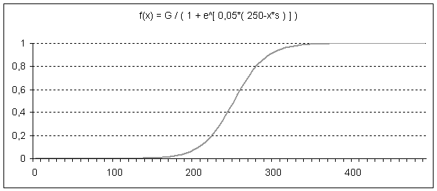
f_logit(x) = G / [1 + e^( k * (a - x) ) ](2)

4.14
The constant factors in the logistic function represent different characteristics of it. First, there is an upper asymptote of the function (G). This is selected to be 1 because in our case the function is used as a weight in the interval between 0 and 1. Second, there is the slope-factor (k) from the turning point, where (k*G/4) is the slope itself. Finally, the position of the turning point at the abscissa (a) can be selected. Now the two remaining constants (k and a) must be valued according to the model. It is assumed that the indirect network effects (INE) have an earlier influence on the decision of the adopters than DNE, but their impact rises slowly. This plays a major role in adapting decisions, because the possibility of using the new knowledge somewhere else is higher (like in the case of QWERTY), and it can be transferred more directly. With 500 adopters as used in the upper simulations, the turning point (a) is selected to be at 150, but it has only a soft slope-factor (k) of 0.02. The graph looks like the following (see Figure 8):

Figure
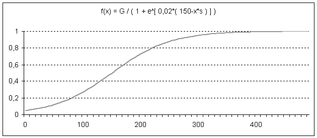
Figure 8. Smooth logistic information diffusion for indirect network effects

4.15
In the case of direct network effects (DNE), a later influence on the decision with a steeper impact is assumed. Although the direct network effects are calculated on the basis of possible network connections using the triangular function, it is important for the weighting whether all those possible connections are already useful for an adopter entering the market. First movers establish a local network without being connected to other local networks. If these networks get connected, both the realized connections and the possibility of sharing increase sharply, as well as the possibility of getting connected to others. Once a large network has developed, almost the total utility is available. With a maximum of 500 adopters, the turning point (a) is selected to be at 250 with a sharper slope-factor (k) of 0.05. The upper asymtote of the function (G) is again 1. The graph looks like the following (see Figure 9):

Figure
Figure 9. Sharp logistic information diffusion for direct network effects

4.16
Of course, other logistic functions are possible in both cases: A product or technology heavily dependent on direct (for example, ’skype’ as a communication program) or indirect network effects (for example, natural gas fuelling stations as a necessary condition for alternative drive engineering cars and depending on them) would show other graphs; in this case, earlier and more steeply rising curves. The issue of small markets can be integrated into this concept as well, by modifying the functions and curves. Although they have an earlier influence on adoption decisions, the results may lead to a market process frozen in the early stages without locking in one technology.
4.17
Now it is important to decide whether both technologies should have the same logistic functions for each direct and indirect network effect or not. Because the technologies are seen as perfect substitutes (as described in the introduction of the Gaussian inclinations) with little differences in characteristics, the equality of the weighting functions is assumed.

Technology A Technology B
G-agenta + vA nA + wA mA (1-a) + vB nB + wB mB
Table 5. Gaussian distributed actors for two technologies
with modified weighted direct and indirect network effects

4.18
To import the logistic weighting into PHP, a function is programed that can calculate the weighting for direct and indirect network effects (see Code 10):

// Calculate logistic y-value
function logit (G, k, a, x) {
f_x = G / (1 + exp(k * (a - x)));
return f_x;
}
Code 10. Logistic function
This pseudo code represents a snippet from the full program only (lines 123-126); a complete
version (with PHP/Winbinder) may be downloaded from here and run under Windows

4.19
The calculation of the direct and indirect network effects then needs to be changed according to the dynamic constants (see Code 11). The modified decision rule from above (see Code 9) does not change, because the results of the network effects are already weighted.

//calculating weighted indirect network effects
INE_a = stack_a * logit(G_u, k_u, a_u, stack_a);
INE_b = stack_b * logit(G_u, k_u, a_u, stack_b);

//calculating weighted direct network effects
DNE_a = (stack_a * (stack_a-1) * (1/2)) * logit(G_v, k_v, a_v, stack_a);
DNE_b = (stack_b * (stack_b-1) * (1/2)) * logit(G_v, k_v, a_v, stack_b);
Code 11. Modified indirect and direct network effects
This pseudo code represents a snippet from the full program only (lines 693-699); a complete
version (with PHP/Winbinder) may be downloaded from here and run under Windows

4.20
Arthur’s implicit assumption of self-reinforcing mechanisms increasing from the very beginning of the process now becomes explicit. The phase of simple random walk towards the lock-in is omitted; it is possible that even the second adopter is crucially influenced by direct or indirect network effects. For adopters with a high inclination, it seems like a random walk, expressing their expected utility mainly through the inclination; indifferent adopters are mainly influenced by direct and indirect network effects, even if they have not yet increased much. A result of these modifications for 500 adopters and 20 simulations looks like the following (see Figure 10, and compared to Figure 4, 5, and 6):

Figure
Figure 10. Distribution with Gaussian adopter, indirect, and direct network effects

4.21
One problem in this process is that the elapsed time is event time and not clock time, as adopters are the relevant unit. If the network effects or the inclination are subject to learning or experience curves, different coefficients, even decreasing, may be the result of the modified model. This modification might be integrated into the logistic functions of the coefficients.

The Application of a Lock-In Dependent from Past Decisions

4.22
One main issue of path dependence is where the lock-in really occurs in comparison to Arthur’s fixed value random walk or his weighted urn market. When simulating a path dependent process, market actors, organizations, and adopters may react, if a lock-in is to be avoided. Additionally, it can be successful as well as devastating for firms acting in a lock-in jeopardized market. Strategies for markets or competition in these contexts may heavily depend on where a lock-in may occur. In Arthur’s processes, the size of the natural inclination determines the event of a lock-in. So, with two separate homogenous groups of adopters equal in size, the utility of the network effects outpaces the natural inclination regarding the adoption decision at the point of lock-in (Leydesdorff & Besselaar 1998; Leydesdorff 2001).
4.23
In the case of adopters with a continuum of natural inclinations, a lock-in function needs to be interpreted in a more complex way. Let us say that, at a probability less than 0.01% for returning to an open state, the market is locked in. If there were only adopters with fixed natural inclinations, there would be only one direct way of returning to an equal market share distribution. This would be reached in the following rounds if each adopter is the one with the preferences for the non-dominant design. But due to the dependence of the decision rule on the Gaussian distributed inclination, the way back needs to be calculated with different combinations of inclinations, and therefore with varying probabilities of returning on each step. So there is more than one possible lock-in point on every curve, resulting in a lock-in band. The distribution of the lock-in points also follows a Gaussian distribution, wherein the mean of all the lock-in points for one curve would result in a lock-in function of the means. Under the conditions of the Gaussian adopter distribution, as well as direct and indirect dynamic network effects, this complex calculation is simulated by the PHP code exhibited in code 12. Of course, the chosen probability of 0.01% is arbitrarily set, but it is, from a statistical and empirical point of view, more plausible than a fixed barrier expressed in absolute numbers as in Arthur’s model.

//Initialize help
help_p_a = 1;

//calculate number of necessary runs to equal market shares
n = stack_a - stack_b;
if (n < 0) {
n = n * (-1);
}

for (i = 1 to n) {
//select Gaussian adopter who is sponsored to take the minor alternative
$pref_a = gauss();
$pref_b = 1-$pref_a;

if(stack_a - stack_b < 0) {
//calculate indirect network effects
INE_a = (stack_a + n) * logit(G_u, k_u, a_u, (stack_a + n));
INE_b = (stack_b) * logit(G_u, k_u, a_u, stack_b);

//calculate direct network effects
DNE_a = ((stack_a + n) * ((stack_a + n) - 1) * (1/2))
* logit(G_v, k_v, a_v, (stack_a + n));
DNE_b = (stack_b * (stack_b - 1) * (1/2))
* logit(G_v, k_v, a_v, stack_b);

help_p_a = help_p_a * ( (pref_a+INE_a+DNE_a) /
((pref_a+INE_a+DNE_a)+ (pref_b+INE_b+DNE_b)) );
}
if(stack_a - stack_b > 0) {
INE_a = (stack_a) * logit(G_u, k_u, a_u, stack_a);
INE_b = (stack_b + n) * logit(G_u, k_u, a_u, (stack_b + n));

DNE_a = (stack_a * (stack_a-1) * (1/2))
* logit(G_v, k_v, a_v, stack_a);
DNE_b = ((stack_b + n) * ((stack_b + n) - 1)
* (1/2)) * logit(G_v, k_v, a_v, (stack_b + n));

help_p_a = help_p_a * ( (pref_b+INE_b+DNE_b) /
((pref_a+INE_a+DNE_a)+(pref_b+INE_b+DNE_b)) );
}

//Decide to interrupt routine if probability to return
//is smaller than given value
if (help_p_a < probab_return) {
break;
}
}
Code 12. Lock-in calculation
This pseudo code represents a snippet from the full program only (lines 721-765); a complete
version (with PHP/Winbinder) may be downloaded from here and run under Windows

4.24
Once again, for 20 simulations with 500 adopters, the asymptotic character of the lock-in functions for both alternatives comes into sight (see Figure 11):

Figure
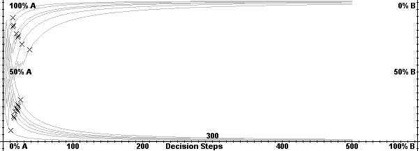
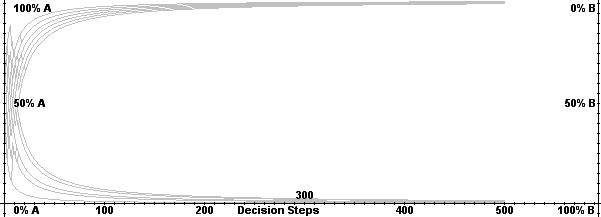
Figure 11. Lock-in function for 20 simulations

4.25
This asymptotic character can be shown more clearly when running this simulation for 10,000 times, marking the lock-in points with dots and not with crosses (see Figure 12). Due to this change, the small lock-in band can now also be observed more clearly where the marked dots were connected after the simulation with a line tool in The Gimp:

Figure
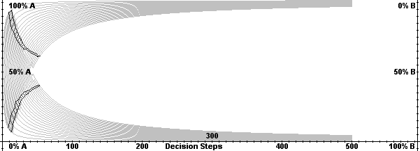
Figure 12. Lock-in band for 10.000 simulations

4.26
We get two lock-in functions, taking the mean within the two asymptotic bands of functions with the fifty-fifty percent line as an attractor. As a result, the lock-in does not depend on a fixed barrier (as in the case of a random walk) or suddenly effective network effects which are higher than the natural inclination (as in the case of the Arthur’s urn model). Finally, the lock-in depends on the market itself. It is estimated with the probability of returning to an equal market share distribution of two alternatives. At the beginning of two competing technologies, the probability of being locked is low. Assuming rising network effects, this probability rises, too. Therefore the lock-in is a relativistic critiria dependent on the possibility of changing something, which may be hard to find in empirical research. Nevertheless, this calculation is more plausible than any other sudden or imprinted point of no return.

* Results and Discussion

5.1
In the following discussion of the results, we refer to the questions provided in the beginning, as well as the limits of this extended model. Finally, the extended model is drawn with its core concepts to extract implications for empirical research on identifying paths and lock ins.

Providing Answers

5.2
The new model is rather complex, and apart from the questions raised in the introduction, it is of some importance where the surplus of this increased complexity lies. This issue will be addressed for each question mentioned in the introduction.
5.3
Processing without Increasing Returns - The first question addressed the problem of what might happen in the process when there are no increasing returns present. This is of some importance, because articles by scholars have tried to address path dependence without such effects (e.g. Rico et al. 2005; Mahoney 2000). Both models, the simple Arthurian model as well as this extended model, can be run without the network effects. Therefore the calculation of the weighted stack or the weighted complexity function can be dropped. As a result, we receive the 50/50 market distribution of a pure random walk process in both cases. In this case, the Gaussian adopter distribution is reproduced in the distribution of market shares of around 50/50. The need for the extended model in the case of no increasing returns is not obvious, but changes in any of the above developed parameters can lead to results that change the expected outcomes dramatically.
5.4
Processing until Lock-in with Increasing Returns - The second question addresses a model of path dependency, where, after the lock-in, the increasing returns might stop. Again, both models, the simple Arthurian model as well as this extended model, can be modified by a condition to switch off the increasing returns after the lock-in (see Figure 13).

Figure
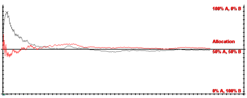
Figure 13. Arthurian and Extended Model without Returns from Lock-in

5.5
In the case of the Arthurian model (red line / lower), the lock-in is equal to the point where the increasing returns start to overweigh the natural inclination. The modification leads to a pure random walk and, of course, to the same result as in the first answer: the same market distribution as in a pure random walk. In the case of the extended model (grey line / upper), the lock-in is not equal to the starting point of the increasing returns. A closer look at single paths of development shows that the increasing returns now drive the process to one of the possible alternatives. When the lock-in occurs and the increasing returns cease, the Gaussian distributed adopters drive the process towards a final random walk. The same output as in the simple model can finally be observed, but the process has a different hape. Finally, a lock-in cannot exist without actively increasing returns. Therefore the extended model helps to clarify that there is no lock-in and no path dependence without increasing returns running all the time.
5.6
Random Dropout of Increasing Returns - The third question targets the problem that, in market processes the, increasing returns might randomly drop for the adopters, due to technological innovation. Again both models, the simple Arthurian model as well as this extended model, can be modified via a condition to randomly drop the increasing returns (see Figure 14).

Figure
Figure 14. Arthurian and Extended Model with Randomly Dropped Returns

5.7
In the Arthurian model (red line / upper) there is, at first, a random phase that turns into an increasing one as soon as network effects are higher than the natural inclination. When the increasing returns drop, the process turns into a random walk process. Finally the same market distribution as in the first answer is reached. In the case of the extended model (grey line / lower), the drop of increasing returns also leads finally to a market distribution like in the random process. The major difference is again that the increasing returns take effect directly from the beginning onwards, and there is no random phase observable in path processes. In addition, the random process after the dropout of the returns takes a decreasing function, rather than the more linear one in the Arthurian model. The lock-in as well as the equilibrium is reached therefore faster with Gaussian distributed actors.
5.8
Aspects for Empirical Research - In contrast to Arthur’s model, where the increasing returns were present in the beginning of the process but have an influence only after the lock-in occurs, there is no need to talk about events without increasing returns regarding this extended model. The first critical juncture or bifurcation point from which the increasing returns start needs to be shown empirically (1). But according to complexity research, the initial conditions for a start of complex path dependent process with reinforcing effects are considered to be hardly determinable (Lorenz 1963). Therefore it would be nice but not necessary to identify the bifurcation point. The second aspect is more important. Here, it is needed to show at least one sort of return that increases the utility of adopters by choosing the alternative, according to the payoff; a self-reinforcement (2). Further empirical work or simulation studies need to show whether power, legitimacy, or only utilitaristic arguments follow the mechanism of self-reinforcement (Beyer 2005). Transforming the increasing characteristics into the adopters’ view (internal view), a decreasing horizon of decision possibilities results as in the organizational model of path dependency (Sydow et al. 2005). The point of lock-in as a third aspect is as hard to identify as the initial conditions, because it depends on the probability to return to an open state. Hence, a relativistic measurement is needed (3). One possible way to measure this is the suggested asymmetry of costs evaluated as a rising barrier (David 1985; Arthur 1988; Arrow 2004), as empirically tested (Strobel & Roedenbeck 2006), or possibly cognitive investments. Contrary to Arthur’s model, this simulation study suggests that increasing returns need to be present after the point of lock-in, too. They are thus the main force supporting hyperstability. As soon as the increasing returns disappear, the path disappears too. This leads into path breaking research, where the activities of newcomers now need to be referred to the dominant increasing returns. Breaking activities then need to support actors’ decisions in order to act against the improbable, but possible, solution (Roedenbeck et al. 2005). Social and hidden costs also need the be regarded concerning path breaking activities because they act against the process (Herrmann-Pillath 2002: 240f.). Graphically, the main empirical aspects of the model can be shown for the external view of increasing market shares (top) and for the internal view of a decreasing variety of choices (bottom). (see Figure 15):

Figure
Figure 15. New Model for Empirical Research

Limits and Further Research

5.9
The new model was derived out of Arthur’s first expressions, but simulation studies discussed some aspects that have not yet been integrated (Leydesdorff & Besselaar 1998): 1) uncertainty, 2) technological leap-frogging, and 3) changes in network parameters.
5.10
Uncertainty - Although we suggested that most adopters do not clearly prefer one technology, the normal distribution can not accomplish the task of introducing uncertainty into this model. Uncertainty means that the probabilities of future adopters for adopting the same technology and the sequence of adopters choosing one or the other technology are not known. So the natural inclination of adopters is not only a Gaussian distributed function, it is also influenced by the prediction of utility maximizing adopters (Neumann & Morgenstern 2004 [1944]). As a result, some of the adopters with the Gaussian selected natural inclinations might wait until a difference between both total utilities (inclination, technology, and network utility and expected network utility) can be confirmed. In the next step, a Poisson distributed waiting function for clock time should be integrated into the model (Härtter 1974). This, of course, would change the logistic functions as well.
5.11
Technological Leap-Frogging - Innovations evolve from new technologies or an improvement of existing technologies. This may lead to a change of the inclination of all adopters towards this improved alternative. Suggesting competing technologies, such ’leap-frogging’ would lead to an end of the simulation, because the assumption of competition of two real alternatives right from the start is no longer fulfilled. There are two possible ways at hand to deal with ’leap-frogging’: 1) Technological leaps take place and could be integrated into the model by changing the coefficients dynamically. But the effect of increasing returns and changing inclinations could be superposed by any other external shock as well. Hence, technological leap-frogging can be simulated with the new model, but shows no new aspects. 2) Technological leaps can also be interpreted as new products. Like in past simulation studies, it would be useful to overlap one simulation with multiple other ones of the same type (for an example with Arthur’s model, see Leydesdorff 2000). But contrary to earlier studies, the change within the adopters’ inclination from the old to the new alternative needs to be regarded more closely. The question whether the change can be interpreted as the beginning of a new simulation or how the increasing returns of the old alternative are overcome by the new ones especially need to be discussed. By this, the less restrictive debate about path creation and breaking can be mathematically addressed (Garud & Karne 2003; Garud & Karne 2001). Nevertheless, the application of the model can be done by modifying existing models of network markets in the literature, for example, the computer industry (Malerba et al 2001).
5.12
Changes in Network Parameters - The determination of the several coefficients in the model is one of the most difficult problems. They are not only estimated in the beginning of the process (as might be done in this model, by using empirical data of comparable cases) but they might change in time. Because there is no empirical evidence for a change of information distribution not according to the stack (as simulated with the logistic functions), this has not yet been integrated but may be if any evidence is found.
5.13
In addition to these aspects, further development of criteria for the coefficients is needed, as well as empirical evidence for the network functions in this simulation. Developing models for evaluating such values can give indiations of a market development with increasing returns. Therefore management instruments can be developed for predicting market processes and behavior.

* Notes

1 This question was mainly addressed in the workshop at the Freie Universitaet Berlin "Measuring Path Dependency - The Social Constructivist Challenge" in September 2005. And this question remains unsolved, according to the final statements at the EIASM-workshop "Organising Paths - Paths of Organising", November 2006.
2 Earlier versions of this paper have been presented at the workshop "Measuring Path Dependency - The Social Constructivist Challenge" held at the Freie Universitaet Berlin, September 2005 and at the EIASM-workshop "Organising Paths - Paths of Organising", November 2006.
3 The programming language used for simulating the model is a standalone version of PHP (www.php.net) combined with the winbinder package (winbinder.org) for graphical in- and output on a Windows 2000/XP platform. All given code snippets are pseudo-code where the references are given with lines according to the original program file that is attached to the publication. Some lines in the program are necessary for the graphical in- and output; they are not discussed here.
4 As the initial decision for the first loop, we define all random numbers higher than 0.5 as a step towards solution A. Let us say that in loop one, the alternative A was selected because the random number was higher than 0.5. In the second round, the condition is that all random numbers higher than 0.33 are decisions towards alternative A reflecting the 2:1 ratio.
5 North (1990) does not reduce the concept of path dependence to the soft version of history matters. He argues that "short-run efforts […] may result in the pursuit of persistently inefficient activities" (S. 100). Before defining this lock-in situation he discusses the self-reinforcing mechanisms that Arthur (1983, 1988) names as a reason for this summarizing argument "history matters" (S. 100).

* References

ACKERMANN R (2001) Pfadabhängigkeit, Institutionen und Regelreform. Tübingen: J. C. B. Mohr (Paul Siebeck).

ARROW K J (2004) Path dependence and economic equilibrium. In Guinnane T W, Sundstrom W A & Whatley W (Eds.). History matters. Essays on economic growth, technology, and demographic change, Stanford: Stanford University Press.

ARTHUR W B (1988) Self-Reinforcing Mechanisms in Economics. In Pines D (Ed.). The Economy as an Evolving Complex System, Reading, MA: Addison-Wesley.

ARTHUR W B (1989) Competing Technologies, Increasing Returns, and Lock-In by Historical Events. Economic Journal, 99. pp. 116-131.

ARTHUR W B (1994) Increasing Returns and Path Dependence in the Economy. Ann Arbor: University of Michigan Press.

ARTHUR W B (1996) Increasing Returns and the New World of Business. Harvard Business Review, July-Aug., pp. 1-10.

ARTHUR W B, Ermoliev Y M & Kaniovski Y M (1983) On Generalized Urn Schemes of the Polya Kind. Kibernetika, 19(1), pp. 49-56.

ARTHUR W B, Ermoliev Y M & Kaniovski Y M (1985) Strong Laws for a Class of Path-Dependent Urn Processes. Paper presented at the: International Conference on Stochastic Optimization, Kiev.

BASS F M (1969) A New Product Growth Model for Consumer Durables. Management Science, 15, pp. 215-227.

BEYER J (2005) Pfadabhängigkeit ist nicht gleich Pfadabhängigkeit! - Wider den impliziten Konservativimus eines gängigen Konzeptes. Zeitschrift für Soziologie, 34(1), pp. 5-21.

BOX G E P & Muller M E (1958) A note on the generation of random normal deviates. The Annals of Mathematical Statistics, 29(2), pp. 610-611.

BRITTON J N H (2004) The Path Dependence of Multimedia: Explaining Toronto’s Cluster. Working Paper - 6th Annual ISRN National Meeting, pp. 13.

BRUGGEMANN D (2002) NASA: a path dependent organization. Technology in Society, 24, pp. 415-431.

CALDAS J C & Coelho H (1999) The Origin of Institutions: socio-economic processes, choice, norms and conventions. Journal of Artificial Societies and Social Simulation, 2(2), https://www.jasss.org/2/2/1.html

COWAN R & Gunby P (1996) Sprayed to Death: Path Dependence, Lock-in and Pest Control Strategies. The Economic Journal, 106(436), pp. 521-542.

DAVID P A (1985) Clio and the Economics of QWERTY. American Economic Review, 75(2), pp. 332-337.

DODSON J A & Muller E (1978) Models of New Product Diffusion Through Advertising And Word-of-Mouth. Management Science, 24(15), pp. 1568-1578.

GARUD R & Karnøe P (2001) Path creation as a process of mindful deviation. In Garud R & Karnøe P (Eds.). Path Dependence and Creation, London: Lawrence Erlbaum Associates.

GARUD R & Karne P (2003) Bricolage vs. breakthrough: Distributed and embedded agency in technology entrepreneurship. Research Policy, 32(2), pp. 277-300.

GOMPERTZ B (1825) On the Nature of the Function Expressive of the Law of Human Mortality, and on a New Mode of Determining the Value of Life Contingencies. Philosophical Transactions of the Royal Society of London, 115, pp. 513-585.

HELFAT C E (1994) Evolutionary trajectories in petroleum firm R&D. Management Science, 40(12), pp. 1720-1747.

HÄRTTER E (1974) Wahrscheinlichkeitsrechnung für Wirtschafts- und Naturwissenschaftler. Göttingen, Vandenhoeck & Ruprecht.

HERRMANN-PILLATH C (2002) Grundriß der Evolutionsökonomik. München: UTB-Wilhelm Fink Verlag.

KEMP J (1999) Spontaneous Change, Unpredictability and Consumption Externalities. Journal of Artificial Societies and Social Simulation, 2(3), https://www.jasss.org/2/3/1.html

LEYDESDORFF L & Besselaar P V d (1998) Competing Technologies: Lock-ins and Lock-outs. In Dubois D (Ed.). Computing Anticipative Systems, New York: National Academy of Physics.

LEYDESDORFF L (2000) The triple helix: an evolutionary model of innovations Research Policy, 29(2000), pp. 243-255.

LEYDESDORFF L (2001) Technology and Culture: The Dissemination and the Potential ’Lock-in’ of New Technologies. Journal of Artificial Societies and Social Simulation, 4(3), https://www.jasss.org/4/3/5.html

LIEBOWITZ S J & Margolis S E (1990) The Fable of the Keys. Journal of Law and Economics, 33, pp. 1-26.

LIEBOWITZ S J & Margolis S E (1995) Path Dependence, Lock-In, and History. Journal of Law, Economics and Organization, 11(1), pp. 205-226.

LIEBOWITZ S J & Margolis S E (2001) The Fable of the Keys. In Margolis S E (Ed.). Winners, Losers & Microsoft. Competition and Antitrust in High Technology, Oakland: The Independent Institute.

LORENZ E N (1963) Deterministic Nonperiodic Flow. Journal of the Atmospheric Sciences, 20(2), pp. 130-141.

MAHONEY J (2000) Path Dependence in Historical Sociology. Theory and Society, 29(4), pp. 507-548.

MALERBA F, Nelson R, Orsenigo L & Winter S (2001) History-Friendly models: An overview of the case of the Computer Industry, Journal of Artificial Societies and Social Simulation, 4(3), https://www.jasss.org/4/3/6.html

NEUMANN J v & Morgenstern O (2004 [1944]) Theory of Games and Economic Behavior. Princeton, NJ: University Press.

NORTH D C (1990) Institutions, Institutional Change and Economic Performance. Cambridge, MA: Cambridge University Press.

PUFFERT D J (2002) Path Dependence in Spatial Networks: The Standardization of Railway Track Gauge. Explorations in Economic History, 39, pp. 282-314.

RICO A, Costa-Font & Power J (2005) Rather Power Than Path Dependency? The Dynamics of Institutional Change under Health Care Federalism. Journal of Health Politics, Policy and Law, 30(1-2), pp. 231-252.

ROEDENBECK M R H, Strobel J C & Tepe M (2005) ’Walking through the Path-Dice: How to Measure the Single Phases of Path Dependency’ Paper presented at the: Measuring Path Dependency - The Social-Constructivist Challenge, Freie Universität Berlin, Berlin, Germany.

ROGERS E M (1983) Diffusions of Innovations. New York, London: The Free Press.

SAHAL D (1981) Patterns of technological innovation. London et al.: Addison-Wesley.

SCHREYÖGG G, Sydow J & Koch J (2003) "Organisatorische Pfade - Von der Pfadabhängigkeit zur Pfadkreation". In Sydow J (Ed.). Managementforschung 13: Strategische Prozesse und Pfade, Wiesbaden.

STERMAN J D (2000) "Path Dependency and Positive Feedback". Business Dynamics, Boston: McGraw Hill.

STROBEL J C & Roedenbeck M R H. 2006. ’How to Shape Markets for Fuel-Efficient Automobiles? Lessons from the Success-Story of Diesel Cars in Germany.’ Paper presented at the: 22nd EGOS Colloquium, Bergen, Norway.

SYDOW J, Schreyögg G & Koch J. 2005. ’Organizational Paths: Path Dependency and Beyond.’ Paper presented at the: 21st EGOS Colloquium, Berlin, Germany.

VERHULST P F (1838) ’Notice sur la loi que la population suit dans son accroissement’. Correspondance mathÈmatique et physique, 10, pp. 113-121.

----

ButtonReturn to Contents of this issue

© Copyright Journal of Artificial Societies and Social Simulation, [2007]