©Copyright JASSS

JASSS logo ----

Thorsten Chmura and Thomas Pitz (2007)

An Extended Reinforcement Algorithm for Estimation of Human Behaviour in Experimental Congestion Games

Journal of Artificial Societies and Social Simulation vol. 10, no. 2
<https://www.jasss.org/10/2/1.html>

For information about citing this article, click here

Received: 19-Jun-2006    Accepted: 20-Nov-2006    Published: 31-Mar-2007

PDF version


* Abstract

The paper reports simulations applied on two similar congestion games: the first is the classical minority game. The second one is an asymmetric variation of the minority game with linear payoff functions. For each game, simulation results based on an extended reinforcement algorithm are compared with real experimental statistics. It is shown that the extension of the reinforcement model is essential for fitting the experimental data and estimating the player's behaviour.

Keywords:
Congestion Game, Minority Game, Laboratory Experiments, Reinforcement Algorithm, Payoff Sum Model, Game Theory, Experimental Economics

* The Investigated Games

Congestion Game I (CI) — The Minority Game

1.1
The first discussed congestion game (CI) is a well known minority game Challet (1997;Challet and Zhang 1998). The minority game is an important example of a Congestion Game. The game can be applied on different situations with social and economic contexts. One can analyse the minority game exemplarily as an elementary traffic scenario in which human participants had to choose several times between a road A and a road B. In each period, the road which was chosen by the minority of players won. This paper reports about the results of laboratory experiments of minority games and a learning algorithm witch simulates the observed human behaviour in these games.

1.2
The minority game is the most important example for a classic non-zero-sum-game and can be applied on different situations with social and economic contests. Imagine two big and famous gold fields in South Africa, near Cape Town and Johannesburg. The diggers heard that a big gold-nugget was found in Johannesburg. From now on every digger went to Johannesburg to dig gold, the city got overcrowded and there was not enough space for all of them, so the profit was very small. The diggers who stayed in Cape Town on the other hand had enough space for their claims. The profit in Cape Town was very high for everybody. This is an example of the minority game, the people who choose the majority got no payoffs, but the people on the minority in Cape Town found enough gold for all of them, so everybody got a payoff.

1.3
The minority game which is also called the El Farol Bar Problem (EFPB) was introduced by Arthur. The setup of the minority game is the following: a number of agents n have to choose in several periods whether to go in room A or B. Those agents who have chosen the less crowded room win, the others lose.

1.4
Later on, the EFBP was put in a mathematical framework by Challet and Zhang, the so-called Minority Game (MG). An odd number n of players has to choose between two alternatives (e.g., yes or no, A or B, or simply 0 or 1). In the literature are many examples where the MG is discussed (Challet 1997;Challet and Zhang 1998;Johnson et al. 1998).

1.5
In this paper we transferred the minority problem into a route choice context. We did minority game experiments at the Laboratory of Experimental Economics (University of Bonn). In these experiments subjects are told that in each of 100 periods they have to make a choice between a road A and road B for traveling from X to Y.

Figure
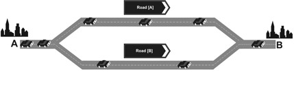
Figure 1. Participants had to choose between a road [A] and a road [B]

1.6
The set-up of the minority game was introduced by Arthur (1991). Newer approaches were done by Challet (1997) and Challet and Zhang (1998). The experimental setup is the following: a number of players n have to choose in several periods whether to go to a place A or B. Those players who have chosen the less crowded place win, the others lose. The number of players in each simulation was 9, the number of periods was 100. The players get a payoff tA or tB depending on the numbers nA and nB of participants choosing A and B, respectively:

tA = 1, tB = 0, ⇔ nA < nB

tB = 1, tA = 0, ⇔ nA > nB

The period payoff was tA if A was chosen and tB if B was chosen. There are no pure equilibria in this game. The pareto-optimum can be reached by 4 players on one and 5 players at the other place.

Asymmetric Congestion Games (CII)

1.7
The second congestion game (CII) is a variation of the minority game: the number of agents in this game was 18, 36, 54, 72 and 90. The number of played periods was in each game 100.

1.8
The period payoff for the 18 player setting was 40 - t with t = tA if A was chosen and t = tB if B was chosen, where tA and tB depend on the numbers nA and nB of participants choosing A and B, respectively:

tA = 6 + 2n and tB = 12 + 3 nB

In the route choice scenario A represents a main road and B a side road. A is faster if A and B are chosen by the same number of people (Selten et al 2003).

1.9
All pure equilibria of the game are characterized by nA = 12 and nB = 6. The equilibrium payoff is 10 units per player and period. The pareto-optimum can be reached by

nA = 11 and nB = 7

1.10
The modified payoff functions for the experiments with 36, 54, 72 and 90 agents are

18λ, λ =2,…, 5,

where

pA = 40 λ = [6 λ + 2 nA]
pB = 40 λ = [12 λ + 3nB]

1.11
Table 1 shows all pure equilibria in the CII depending on the number of players.

Table 1: Pure equilibria in CII. The equilibria depend on the number of participating agents

Number of PlayersEquilibrium
AB
18126
362412
543618
724824
906030

In the case of CII, place A and place B are understand as a road with high capacity (main road) and a road with low capacity (side road) and tA and tB as travel times.

Experimental Set-up of CI and CII

1.12
Each of the games CI and CII with 9 and 18 persons were played 6 times with students at the Laboratory of Experimental Economics in Bonn. Additionally CII was played 1 time with 36, 54, 72 and 90 students. Subjects are told that in each period they have to make a choice between A and B. The subjects of the CII set-up did not know the payoff function. They were told that if A and B are chosen by the same number of people, subjects who had chosen A get a better payoff than subjects who had chosen B. At the end of an experiment, each participant was paid an amount in Euro proportional to his cumulated payoff sum he had reached over the 100 periods. The experimental data statistics are listed and compared with simulation results in section 4.

* Reinforcement Learning

Reinforcement Algorithm with Pure Strategies

2.1
The reinforcement algorithm with pure strategies already described by Harley (1981) has been used extensively by Roth and Erev (1995) in the experimental economics literature. The convergence in games with pure strategies was analyzed by Laslier and Walliser (2005). Selten et al. (2003; 2007), Helbing et al (2002) and Helbing (2004) used a reinforcement model in a traffic context. Figure 2 explains the original reinforcement algorithm.

2.2
We are looking at player i who has to choose among n pure strategies 1, … ,n over a number of periods t, t=1 … T. The probability that "strategy x is chosen by player i" is proportional to its "propensity" qti,x. In period 1 these propensities are exogenously determined parameters. Whenever the strategy x is used in period t, the resulting payoff atx is added to the propensity if this payoff is positive. If all payoffs are positive, then the propensity is the sum of all previous payoffs for this strategy plus its initial propensity. Therefore one can think of a propensity as a payoff sum.

Figure
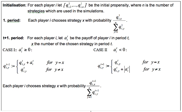
Figure 2. Reinforcement algorithm

The Empirical Foundation for an Extended Reinforcement Model

2.3
The only pure strategies in CI and CII are "place A" and "place B". These strategies do not represent a player's belief about the other participant's behaviour. In our extended model we add two further strategies which include the consideration of players about the others based on the last period's payoff. In CI a "bad" payoff could obviously be defined by 0 and a "good" payoff by 1. In CII with 18λ, λ=1,…,5 players, the pure equilibrium payoff is ε=10λ. Payoffs perceived as "bad" tend to be below ε and payoffs perceived as "good" tend to be above ε. Accordingly we classified the strategy of a subject as direct if there is a change (stay) after a payoff smaller (greater) than 10λ. The opposite strategy is classified as contrarian.

Measuring Direct and Contrarian Strategies

2.4
For each subject let c- (c+) be the number of times in which a subject changes from A to B or from B to A when there was a bad (good) payoff in the period before. And for each subject let S- (s+) be the number of times in which a subject stays on the same place when there was a bad (good) payoff in the period before.

2.5
For each subject in the experiments CI and CII, a Yule coefficient Q has been computed as follows:

Yule's Q

The Yule coefficient has a range from -1 to +1. In the rare cases that a subject never (in each period) changes his last choice, we defined Q = 0 because the decision of such a subject does not depend on the last period payoff. A subject with Yule coefficients below -.5 could be understood to be classified as direct and subjects above +.5 as contrarian.

Extended Reinforcement Learning

2.6
In our simulations of CI 9 agents, respectively of CII 18, 46, 54, 72, 90, agents interact for 100 periods just like in our experiments described in section 3. In CI and CII each player has two pure strategies:
Place A:This strategy consists in taking A.
Place B:This strategy consists in taking B.
After the first period in each of the two games (CI) and (CII) the two extended strategies direct and contrarian are available:
(CI) direct:If the payoff of a player is 1, then the player stays on the same place last chosen. If his payoff is 0, the players changes (from A to B or from B to A).
(CI) contrarian:If the payoff of a player is 1, then the player changes (from A to B or from B to A). If his payoff is 0, the players will stay on the same place.
(CII) direct:This strategy corresponds to the direct response mode. The payoff of a player is compared to his median payoff among his payoffs for all periods up to now. If the present payoff is lower then this median payoff, then the place is changed. If the payoff is greater than this median payoff, the player stays on the same place as before. It may also happen that the current payoff is equal to the median payoff. In this case, the place is changed if the number of previous payoffs above the median is greater than the number of previous payoffs below the median. In the opposite case, the place is not changed. In the rare cases where both numbers are equal, the place is changed with probability ½.
(CII) contrarian:A player who takes this strategy stays on the last chosen place if his current payoff is smaller then the median payoff among this payoffs for all previous periods, and he changes the place in the opposite case. If the current payoff is equal to this median payoff, then he changes the place if the number of previous payoff below the median payoff is greater then the number above the median payoff. If the numbers of previous payoff below and above the median payoff are equal, the place is changed with probability ½.
The strategies direct and contrarian are necessary to be represented in the simulations for fitting the experimental data. They appear in the simulations as the result of an endogenous learning behaviour by which initially homogeneous subjects become differentiated over time.

Initial Propensity

2.7
The difficulty arises that the initial propensities must be estimated from the empirical data. For each game CI and CII we did this by varying the initial propensities for the strategies place A and place B over all integer values from 1 to 120 and the initial propensities for the strategies direct and contrarian over all integer values from 0 to 120. For each initial propensity we tested 1000 simulations. To show the general behaviour of the simulations, Figures 4 to 6 show several selected statistical parameters depending on the initial propensities listed in figure 3. The numbers refer to the strategies place A, place B, direct and contrarian in this order.

Figure
Figure 3. Initial Propensities

2.8
One could see in figure 4 that, for each simulation run and each initial propensity the mean number of agents on place A is close to 4.5. The convergence to the theoretical mixed equilibrium was already observed in the simulation data of Roth & Erev (1995).

Figure
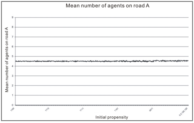
Figure 4. Number of players on A

2.9
The standard deviation of the number of players on place A per period (figure 5) is correlated to the number of changes (figure 6) per periods. It got the highest values with propensities from the set I1. In this cases the strategy direct is present and contrarian is absent. The strategy directly forces changes after a "bad" payoff 0, which is the most frequent in the majority game.

Figure
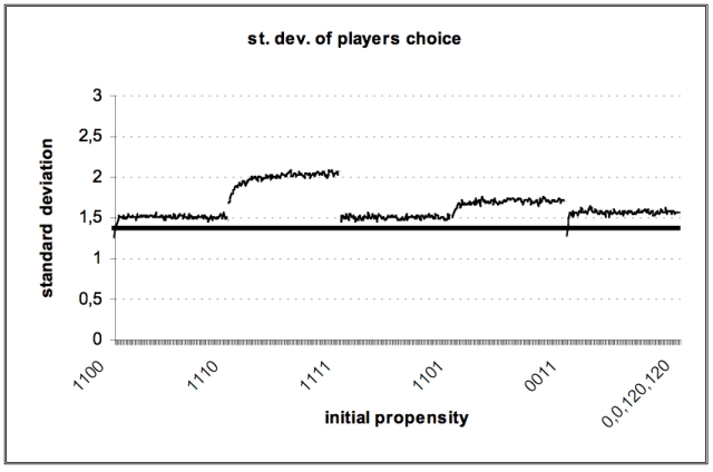
Figure 5. Standard deviation of number of players on A

Figure
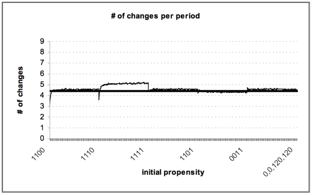
Figure 6. Number of changes per period

2.10
Players with high Yule-coefficients in the experiments are assigned to the direct type; this appears also in the figure 7. For the initial propensities, in which no contrarian change behaviour is implemented, for example (1110), step high Yule-coefficients up. For the initial propensities, in which the contrarian behaviour is favoured, for example (1101), all values of the Yule-coefficients are negative.

Figure
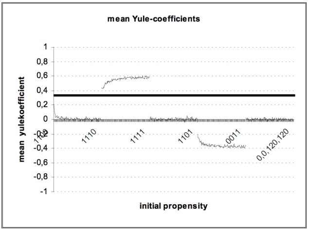
Figure 7. Mean Yule-coefficients

Similar results could be obtained by investigations of the initial propensities for simulations of CII.

* Experimental Statistics and Simulation Results

CI with 9 Players

3.1
For each propensity vector q1, …, q4 ∈ {1, …, 120}2 × {0, …, 120}2 we ran 1000 simulations according to the experiments with 100 periods. The numbers of the propensity vector refer to the strategies place A, place B, direct and contrarian in this order. We compared the mean values of each of the 1000 simulations of 6 statistical variables which are listed in table 2 with minimum and maximum values of the experimental data.

3.2
There were three parameter combinations which satisfied the requirement of yielding means for the six variables between the minimal and maximal experimentally observed values. This was the parameter combination (1,1,2,1) and (2,2,1,1) and (3,3,4,2).

Table 2: CI — 9 Players - Experimental minima & maxima vs. simulation means

CIExperiment
Simulations
Experiment
Minimum{1,1,2,1}{2,2,1,1}{3,3,4,2}Maximum
Player on A [mean]4,194.484.504.544.74
Player on A [standard deviation]0.671.451.481.501.50
Changes [mean]0.594.324.184.515.17
Period of last Change54.4496.1197.6797.4498.11
Yule Q [mean]-0.010.100.040.140.87
Yule Q [standard deviation]0.330.500.400.350.76

3.3
Additionally we could show that the vector (1,1,2,1) minimizes the sum of normalized quadratic deviations of experimental data and simulation results of the six variables. The quadratic deviations where normalized by division by the standard deviations of the experimental results over the treatments. Figure 8 shows the quadratic deviations of the best initial vectors from the average experimental data.

Figure
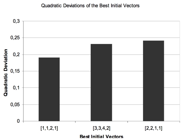
Figure 8. Quadratic deviations of the best initial vectors from the average experimental data

3.4
The parameter combinations seem to be reasonable vectors of initial propensities. There is no difference between place A and place B. It is clear to see that the vectors have the same propensities for both places. In two of the three vectors the propensity of the direct mode is greater than the value of the other propensities. The higher initial value for the direct strategy and the smaller value of the contrarian strategy represent the ratio of the experimental data referring to the player types (Chmura & Pitz 2006).

3.5
It is remarkable that no initial propensities which contain only pure strategies fit the experimental data. We want the simulation model as easy as possible, therefore all experimental players start with the same propensity vector combination in one simulation. As in the experiments the agents become differentiated over time (see figure 10).

CII with 18 Players

3.6
In set-up CII with 18 players, we got only one parameter combination from the set {0, …, 120}2 × {0, …, 120}2which satisfied the requirement of yielding means for the six variables between the minimal and maximal experimentally observed values. This was the parameter combination (4,3,3,2). In table 3, we compared the mean values of each of the 1000 simulations of 6 statistical variables which are listed in table 3 with minimum and maximum values of the experimental data.

3.7
Additionally we could show that the vector (4,3,3,3) minimizes the sum of normalized quadratic deviations of experimental data and simulation results of the six variables. The quadratic deviations where normalized by division by the standard deviations of the experimental results over the treatments.

3.8
Figure 9 shows the distribution of the mean player on B for the simulated vector (4,3,3,2) in 1000 simulations.

Table 3: CII — 18 Players: experimental minima & maxima vs. simulation means

CIIExperimentSimulations Experiment
Minimum{4,3,3,2}Minimum
Player on B [mean]5,855,956,17
Player on B [standard deviation]1,591,651,99
Changes [mean]4,625,175,38
Period of last Change64,7883,7390,39
Yule Q [mean]0,110,140,39
Yule Q [standard deviation]0,530,610,75

Figure
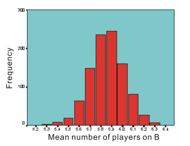
Figure 9. Distribution of the mean number of players on B for the simulated vector (4,3,3,2) in 1000 simulations

3.9
At the beginning of the game the players know that the capacity of A is greater than the capacity of B. It seems to be reasonable to suppose that at least in the beginning the pure strategies A and B have a greater propensity sum than direct and contrarian. Like in CI, no initial propensity which contains only pure strategies fits the experimental data. Further on it seems reasonable that the initial value for A is greater than the initial value for B. The reason for this is the game theoretical equilibrium in the experiments with human players. The equilibrium shows a higher value for A (equilibrium in the experiments with 18 players was A:12 B:6 ). In the experiments occur more direct player types 40% and less contrarian player types 20% (Selten et al 2003). This ratio could be found in the simulations, where the 3 represents the initial value for the direct strategy and 2 represents the initial value for the contrarian strategy.

Simulations of CII with 18, 36, 54, 72, and 90 Players

3.10
Finally we compared the mean of six statistical variables of 1000 simulations with 18, 36, 54, 72, and 90 players with experiments of the same number of players. For simulations with 18λ players we used the initial propensities λ · (4,3,3,2), λ=2, … , 5. The vector (4,3,3,2) has been determined above.

3.11
Additionally we could show that the vector (4,3,3,3) minimizes the sum of normalized quadratic deviations of experimental data and simulation results of the six variables. The quadratic deviations where normalized by division by the standard deviations of the experimental results over the treatments.

Table 4: CII — Experimental means (E) vs. Simulation means (S)

Statistical Data CIIData SourceNumber of Players
1836547290
Mean (# players on B)E5.9812.2117.9824.230.02
S5.9511.9117.923.8329.02
st. Dev. (# players on B)E1.782.643.244.545.02
S1.652.393.043.784.58
Mean (# of place changes)E4.8211.3515.5722.7626.02
S5.1710.0715.9821.3223.04
Mean (last place changeE8182868988
S8489848890
Mean (Yule-coefficient)E0.280.140.220.20.24
S0.140.160.150.150.16
st. Dev. (Yule-coefficient)E0.580.580.580.570.6
S0.610.540.540.520.56

* Conclusion

4.1
We have run simulations based on a payoff sum reinforcement model. We applied this model on two similar experimental set ups CI and CII. Simulated mean values of six variables have been compared with the experimentally observed minimal and maximal of these variables. The simulated means were always in this range. Only four parameters of the simulation model, the initial propensities, were estimated from the data. In view of the simplicity of the model, it is surprising that one obtains a quite close fit to the experimental data. With a linear transformation of the initial propensity, the simulations fit experimental results with a higher number of players.

4.2
Two response modes can be found in the experimental data, a direct one in which changes follow bad payoffs and a contrarian one in which changes follow good payoffs. One can understand these response modes as due to different views of the causal structure of the situation. If one expects that A is crowded in period t, and A is likely to be crowded in period t+1 one will be in the direct response mode. But if one thinks that many people will change in the next period because it was crowded today, one has reason to be in the contrarian response mode.

4.3
The strategies direct and contrarian are necessary to be represented in the simulations for fitting the experimental data. They appear in the simulations as the result of an endogenous learning behaviour by which initially homogeneous subjects become differentiated over time. A sample simulation for 9 players over 1000 periods is shown in figure 9. Each player has a specific colour. The grey line indicates the separation of the player's payoff sums at period 100.

4.4
It is surprising that a very straightforward reinforcement model reproduces the experimental data as well as shown by table 4. Even the mean Yule coefficient is in the experimentally observed range in spite of the fact that at the beginning of the simulation the behaviour of all simulated players is exactly the same. It is not assumed that there are different types of players.

Figure
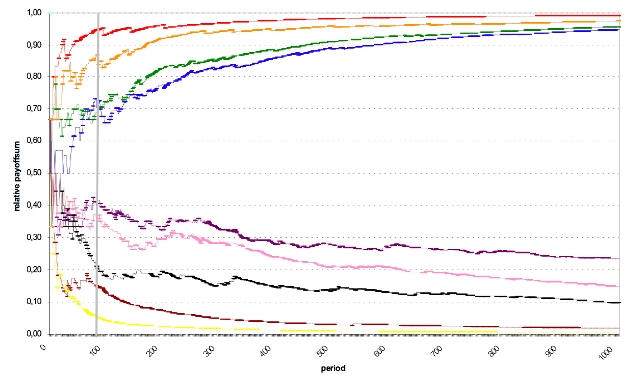
Figure 10. Example simulation shows the relative payoff-sum for each of the 9 players over 1000 periods

* Appendix

A.1
Figures 11-16 illustrate the experimental means in comparison to the simulated means of table 4. Black boxes represent the simulated values and white boxes, the empirical data.

Figure
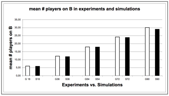
Figure 11. Mean Number of Players on B in Experiments and Simulations

Figure
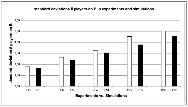
Figure 12. Standard Deviation number of Players on B in Experiments and Simulations

Figure
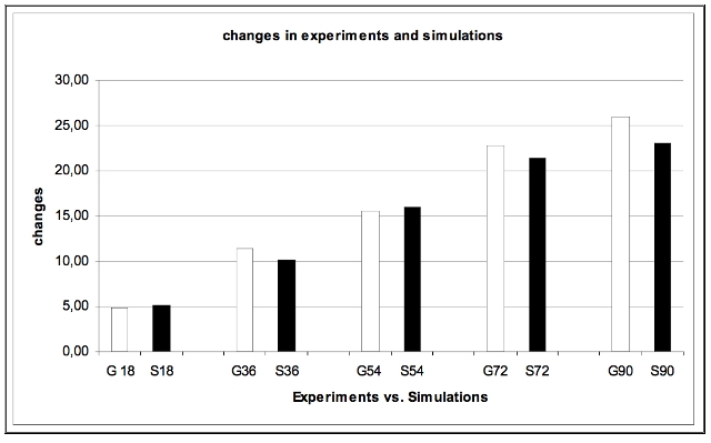
Figure 13. Number of Changes in Experiments and Simulations

Figure
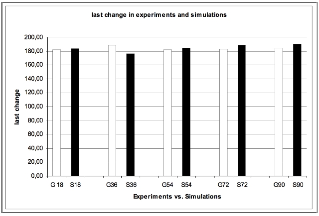
Figure 14. Last change in experiments and simulations

Figure
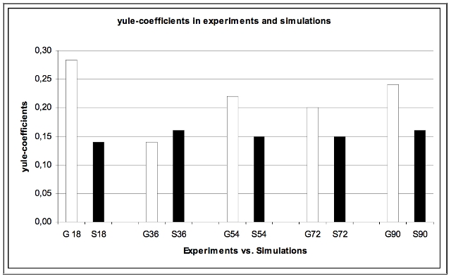
Figure 15. Mean Yule-coefficients in experiments and simulations

Figure
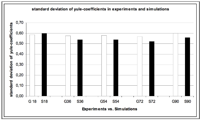
Figure 16. Standard Deviation of Yule-coefficients in Experiments and Simulations


* Acknowledgements

We are grateful to the BMBF and the DFG for financial support. We also like to thank Sebastian Kube for the valuable help and the programming.

* References

ARTHUR W. B. (1991) Designing economic agents that act like human agents: A behavioural approach to bounded rationality. Amer. Econ. Rev. Papers Proc. 81 May, 353-359.

CHALLET, D., Zhang, Y.-C., (1997) Emergence of cooperation and organization in an evolutionary game. Physica A 246, 407-418.

CHALLET , D., Zhang, Y.-C., (1998) On the minority game: Analytical and numerical studies. Physica A 256, 514-532.

CHMURA, T.., Pitz, T., (2006) Successful Strategies in Repeated Minority Games. Physica A 363, 477-480.

HARLEY, C. B. (1981) Learning in Evolutionary Stable Strategies, J. Theoretical Biology 89, 611-633.

HELBING, D., Schönhof, M., Kern, D. (2002) Volatile decision dynamics: Experiments, stochastic description, intermittency control, and traffic optimization. New Journal of Physics 4, 33.1-33.16.

HELBING, D. (2004) Dynamic decision behavior and optimal guidance through information services: Models and experiments in: M. Schreckenberg and R. Selten (eds.) Human Behaviour and Traffic Networks (Springer, Berlin) Pages 47-95.

JOHNSON, N. F., S. Jarvis, R. Jonson, P. Cheung, Y. R. Kwong, and P. M. Hui (1998) Volatility and agent adaptability in a self-organizing market. Physica A 258, 230-236.

LASLIER , F, Walliser, B., (2005) Reinforcement Learning Process in Extensive Form Games Game Theory, 33, 219-227.

ROTH, A.E., Erev, I. (1995), Learning in extensive form games: Experimental data and simple dynamic models in the intermediate term, Games and Economic Behavior 8, 164-212.

SELTEN, R., Schreckenberg, M., Pitz, T., Chmura, T., Kube, S. (2003) Experiments and Simulations on Day-to-Day Route Choice Behaviour, CESIFO Working Paper No. 900, Munich.

SELTEN, R., Chmura, T., Pitz, T., Kube, S., Schreckenberg, M. (2007) Commuters Route Choice Behaviour, Games and Economic Behaviour 58, 394-406.

----

ButtonReturn to Contents of this issue

© Copyright Journal of Artificial Societies and Social Simulation, [2007]