Giorgio Brajnik and Marji Lines: Qualitative modeling

Giorgio Brajnik and Marji Lines (1998) 'Qualitative modeling and simulation of socio-economic phenomena'

Journal of Artificial Societies and Social Simulation vol. 1, no. 1, <https://www.jasss.org/1/1/2.html>

To cite articles published in the Journal of Artificial Societies and Social Simulation, please reference the above information and include paragraph numbers if necessary

Received: 23-Oct-1997 Accepted: 13-Dec-1997 Published: 3-Jan-1998

A version of this article in Portable Document Format (PDF) is also available. The PDF version is recommended if you want to print the article to a laser printer.

Abstract

This paper describes an application of recently developed qualitative reasoning techniques to complex, socio-economic allocation problems. We explain why we believe traditional optimization methods are inappropriate and how qualitative reasoning could overcome some of these shortcomings. A case study is presented where an authority is expected to devise a policy that satisfies certain constraints. We describe how sets of rules of thumb implementing such a policy can be analyzed and validated by the decision maker using a program which automatically builds and simulates qualitative models of the underlying dynamical system. Such a program constructs and simulates models from incomplete descriptions of initial states and functional relationships between variables. We show that it nevertheless gives sufficient information to the decision maker.

Keywords:

qualitative modeling, qualitative reasoning, decision making, allocation

Introduction

1.1: National and international authorities must make difficult policy decisions regarding socio-economic problems which are complex, highly interrelated, and subject to uncertainty and external disturbances. Analytical and simulation models have proven useful in helping decision makers to understand the processes involved in these complex problem/policy contexts (for example, the Law of the Sea agreement (Sebenius, 1984)). In this paper we describe a first attempt to apply qualitative reasoning techniques to model the following problem: a central authority must determine an allocation of national income between consumption, capital investment, social services and anti-pollution activity in order to ensure a sustainable time-path for society.
1.2: A typical model from environmental economics for our case could be represented as an ordinary differential equation including two state variables which influence welfare (utility): per capita consumption (i.e., the proportion of the gross national product "consumed" by a member of the society) and an index of environmental quality (representing the amount of pollution present in the natural environment). In addition, state variables would be subject to constraints: consumption cannot be greater than production, and other environmental constraints may be related to the exhaustion of non-renewable energy sources or to the pollution level endangering the life support services of the environment, for example. The solution of the problem, depending on its formulation, would provide an authority with time-paths for (perhaps optimal) energy-use, anti-pollution activity, emission taxes, incentive schemes for investment in green technology.
1.3: In this paper we propose the use of an alternative method, that of qualitative modeling and simulation techniques recently developed within the field of Artificial Intelligence to formulate and analyze this kind of problems. The benefits are that certain modeling activities can be automated and the user can easily set up different "what-if" analysis scenarios. Secondly, the simulation techniques are suited to the study of systems that are only partially known. The simulators cope with this incomplete knowledge by producing a concise qualitative description of the all the possible outcomes, which may branch at points where the information is ambiguous. This coverage guarantee is then extremely useful in problems of designing a control policy since the predicted outcomes would necessarily contain any unwanted trajectories, that can therefore be detected, triggering a revision of the control policy included in the model. In addition, before applying numerical methods one has to resolve the incompletely specified functional relationships among variables of the system. This may lead to a costly activity of quantitative model formulation and parameter identification. Qualitative simulation techniques can be used as a preliminary step in analyzing the consequences of certain qualitative relationships between variables.

Advantages Of Qualitative Reasoning

2.1

In the field of environmental economics much of the theoretical modeling activity employs the optimal control framework based on Pontryagin's maximum principle (e.g. Siebert, 1987). The goal is to find values for the state variables that maximize (or minimize) an objective function while at the same time satisfying a set of constraints. The method of Lagrange multipliers can then be used to set up a variational calculus problem.

2.2

Economists tend to be interested in equilibrium (steady state) solutions obtained by setting time derivates to zero and hence transforming the differential system into a system of algebraic equations. However, even equilibrium systems, in the presence of nonlinear relations and/or more than two state variables, are difficult to solve. Thus theorists frequently apply techniques of comparative statics rather than solve for the trajectories of interesting variables. For example, one might determine the direction of change of the equilibrium environmental index if the discount rate is higher or lower than hypothesized, rather than solve for the optimal time-path of the environmental index.

2.3

Let us suppose a steady state solution exists and can be determined. The optimal solution will be sensitive to the hypothesized parameter values and, of course, to the specific functional forms adopted in the model. However, the information set often provided on the hypothesized implicit functional forms for production and welfare includes the signs of the first and second partial (and perhaps cross-partial) derivates. If explicit functional forms are volunteered they are usually chosen for characteristics that compare favorably to real life observations as well as mathematical simplicity. Most often power functions are assumed whose coefficients are given a range rather than an exact value.

2.4

From this brief outline of the approach we can summarize four objections to the use of the constrained control framework in policy analysis of real world problems.

Solvability.: The rarity of worked-out solutions in applications to economic policy problems suggests that it may not be a practical technique for studying such problems (difficulty in solving nonlinear systems with possibly more than two state variables).
Complete knowledge.: The precision of the solution method is overwhelmed by necessary imprecision in the hypotheses (should a solution be determined for a specific model, new solutions will have to be determined when studying alternative assumptions that imply changes in functional forms).
Full certainty.: Once a decision on the policy to be adopted, it is assumed that the dynamics of the modeled system remain certain and unchanged over the control horizon, typically infinity, which is rather unrealistic.
Optimization.: The whole policy rests on optimization. If that fails, there are no obvious guidelines for allocating resources.

2.5

We believe that Qualitative Reasoning (QR) techniques (Faltings and Struss, 1992, Kuipers, 1994) meet these objections.

Solvability.: The goal of the analysis is not a unique analytical solution. We make use of simulation to follow all possible state trajectories with the goal of formulating policies able to keep these trajectories within certain limits.
Complete knowledge.: Qualitative models can be based on extremely weak assumptions on the functional form relating two or more variables in a differential equation and yet provide useful results. In addition, numeric information in terms of ranges for parameters and constants and envelopes for functional forms can be added to the model, restricting the possible trajectories. Often, the more knowledge available, the tighter the boundaries and the fewer the qualitatively different trajectories.
Full certainty.: Simulation methods do cope with uncertainty in states and models and propagate it across time up to any horizon of interest, finite or infinite.
Optimization.: Allocation decisions can be informed by analysis of the predicted trajectories of the system. These could serve as guidelines in policy choice. Instead of focusing (only) on optimization using a perhaps oversimplified model, decision makers could focus on inadmissible trajectories and find corrective actions to prevent them from occurring.

2.6

A further advantage of studying non-optimal trajectories in this context is that the entire spectrum of dynamic behavior is permitted and analyzed, not just that described by equilibrium and transition to equilibrium. This should be a better base from which to make policy recommendations for the systems with complicated trade-offs which are inherent to the analysis of economic growth and environmental quality.

Qualitative Modeling And Reasoning

3.1

Two research areas in the Qualitative Reasoning field are particularly suited to deal with dynamic allocation problems, namely: automated modeling and qualitative simulation.

3.2

Automated modeling aims at developing programs which construct models of the system under study and support the human modeler during model management (i.e., a wide spectrum of activities encompassing problem identification and formulation, model creation, implementation and validation, solution of the problem and its interpretation). Qualitative simulation (Kuipers, 1994) enables computers to simulate dynamical systems and to yield useful predictions even in those cases where only very rough and incomplete descriptions of systems exists. A recent research branch called compositional modeling (Falkenhainer and Forbus, 1991, Iwasaki and Low, 1991, Farquhar, 1994) aims at integrating these two functionalities into programs that take as input a (reusable) model of the domain and a description of a specific situation, and produce predictive models and their predictions.

3.3

Automated modeling and qualitative simulation are key ingredients for tackling socio-economic problems that can be conceived in terms of a set of interacting processes based on continuous variables.

3.4

Compositional modeling offers the means to represent in a modular (hence reusable) way fragments of equations that are automatically composed into coherent models on the basis of a description of a simulation scenario. In this way building different models for analyzing different scenarios becomes a relatively easy task, that builds on previous work. Additionally, the capability of these kind of simulators to monitor the simulation and detect the situations in which the boundary of the model validity region is hit, enables the user to analyze scenarios where more than one model has to be used. Compositional modeling programs cope automatically with such a model switching.

3.5

There are two main benefits deriving from the use of qualitative simulators. First is the ability to deal with non-parametric uncertainty, that is uncertainty that is associated to functional relationships (where analytical descriptions and numerical information about a function are missing), instead of being simply included in state/parameter descriptions. Second is the abstraction that qualitative simulation is based upon. The model that is used is a compact representation of a large family of ordinary differential equations, and the simulation results include the solutions of all the instances of the qualitative model.

3.6

In the following of this section we provide a brief description of some of the tools and notions that are most relevant to our work. We start from the underlying qualitative simulator and then move to the model building and simulation tool.

3.7

We provide here a brief description of QSIM; for a deeper discussion and for a thorough overview of applications of QSIM we suggest reading (Kuipers, 1994).

3.8

The input to QSIM is a qualitative differential equation (QDE) which specifies:

a set of variables (continuously differentiable functions of time);
a quantity space for each variable, specified in terms of a totally ordered set of symbolic landmark values;
a set of constraints expressing algebraic, differential or monotonic relationships between variables.

3.9

A QDE is an abstract description of a set of ordinary differential equations. The abstraction is achieved in two ways. Variables takes values from the totally ordered set of symbolic landmarks. Each landmark represents an unknown real number. For example, the starting and equilibrium prices of a demand-supply market model can be represented as two landmarks, whose real value is unknown, for the variable price. Secondly, monotonic relationships can be specified between variables, like expressing that price levels are monotonically increasing with respect to demand. Such a relation is an abstraction of an entire family of (linear and nonlinear) functions. The only requirement is that functions are smooth and that their derivatives have certain signs.

3.10

The output of QSIM is a set of behaviors. Each behavior is a sequence of states, where a state is a mapping of variables to qualitative values. A qualitative value represents the (qualitative) magnitude of the variable (i.e., either a landmark or the open interval between a pair of adjacent landmarks) and the direction of change of the variable (i.e., the sign of its time derivative, represented as dec, std, inc). Each state in a behavior describes either a time point or an open temporal interval. Time is treated as another qualitative variable, whose landmarks are automatically generated by QSIM as critical points of other variables are identified.

3.11

A monotonic function constraint represents an infinite set of real valued functions. It has the general form

where each . Its meaning is given in terms of the subset of continuous differentiable functions ( stands for the set of real numbers extended with positive and negative infinity):

3.12

For example, to specify that price level (P) depends simultaneously on demand (D) and offer level (O), and it increases with demand and it decreases with offer, the following constraint can be used:

3.13

Simulation is based on a constraint satisfaction scheme: (i) successor states are generated by propagating variables' values according to continuity alone; (ii) successor states are filtered using constraints and global criteria (e.g., unreachability of certain landmarks, finite time for covering infinite distance) to decide which states are admissible and which are inconsistent.

3.14

QSIM produces zero or more qualitative behaviors that represent all the possible trajectories from the initial state of all the instances of the QDE (see figure 1).

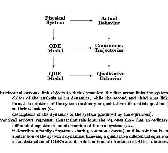
Figure 1: Qualitative simulation uses abstraction to cope with incomplete knowledge

3.15

Hence QSIM is a sound tool. QSIM may yield too general answers, though, being unable (because of the coarseness of the qualitative representation) to remove from the output all the behaviors that are mathematically impossible (spurious behaviors). QSIM is said to be therefore incomplete. To reduce the number of spurious behaviors several extensions have been added to QSIM, each contributing to a significant reduction (yet not a complete elimination) of spurious behaviors.

3.16

One of these extensions enables semi-quantitative simulations to be performed. That is, the basic qualitative representation is augmented: each landmark may be bounded with a numeric upper and lower bound, and each monotonic function constraint may be bounded with a functional upper and lower bound (envelope).

3.17

The semantics of envelopes is easily understood in terms of set of functions. As previously seen, any monotonic constraint is an abstract description of a set of functions. An envelope for a constraint restricts the set of functions that are associated to a constraint to those that are bounded by the envelope.

3.18

On the basis of numeric envelopes associated to monotonic constraints, semi-quantitative simulators augment their predictions with numeric bounds attached to each variable's value in each state. Such an information is then used to rule out those behaviors that, although being consistent with the qualitative differential equation, violate some numeric bound.
Two techniques have been developed for implementing such extension to qualitative simulation. The static envelopes technique developed in (Berleant and Kuipers, 1988) propagates bounds (using algebraic constraints or envelopes) throughout each time-point state and then uses the mean-value theorem to constrain the values across time, for time-interval states. The more recent dynamic envelopes technique (Kay and Kuipers, 1993) constructs extremal equations for the derivative of each state variable¹. These extremal equations are then numerically integrated to provide bounds on variable values across time intervals. Neither technique strictly dominates the other. As a result, the bounds provided by the two methods may be intersected, yielding sometimes stronger predictions than either alone (Kay, 1996b, Kay, 1997).

3.19

SQPC (Semi-Quantitative Physics Compiler) (Farquhar and Brajnik, 1994, Brajnik, 1995) is an implemented approach to modeling and simulation that performs self-monitoring simulations of incompletely known, dynamic, piecewise continuous systems. SQPC automatically constructs a model, simulates it, and monitors the simulation in order to detect violations of model assumptions; when this happens it modifies the model and resumes the simulation. SQPC is built on top of the QSIM qualitative simulator.

3.20

The input to SQPC is a domain model and scenario specified in the SQPC modeling language. A domain model consists of:

A taxonomy of entity types: a hierarchy of types of objects and associated relationships, called structural relations. Types denote sets of objects, and the (built-in) IS-A relation represents set inclusion. For example, IS-A(funded-activities, activities) states that funded activities are a particular case of activities. The user can define domain-dependent relationships, such as supports(societies, funded-activities) meaning that in a society certain funded activities may take place.
A set of quantity types: each quantity type is an attribute of tuples of entity types which maps their instances onto real-valued functions. More specifically, a quantity type QT maps a tuple of entity types ( ) to a set of functions, mapping time ( ) into real numbers. A quantity Q, instantiation of some QT on is a specific function of time:

For example, one can define the quantity type capital(productions)). If car-manufacturing is an instance of productions, then capital(car-manufacturing) is a specific function, mapping time to an amount of money. If Q is a quantity then the term derivative(Q) denotes the quantity representing the time derivative of Q.
a set of quantified definitions, called model fragments, each of which describes some aspect of the domain, such as physical laws (e.g., natural abatement of pollution), processes (e.g., industrial production), mechanisms (e.g., investment rules), and entities (e.g., population, environments). The idea is to represent separate "pieces" of models and equations that can be automatically combined into many different complete models, as opposed to provide already "packaged" models. Each model fragment applies whenever there exists a set of participants for whom the stated conditions are satisfied. The specific system or situation being modeled is partially described by the scenario definition, which lists a set of objects that are of interest, some of their initial conditions, relations that hold throughout the scenario, and boundary conditions.
Influences are compositional relations between variables that are particularly convenient for asserting fragments of information that can be composed into constraints. Three kinds of influences are supported by SQPC.
An instantaneous influence such as means that in the absence of countervailing influences, an increase in X causes an increase in Y. Furthermore, once we determine the set of influences affecting Y, Y is functionally determined by the influencing variables.
Algebraic influences provide additional information on the form of the function f. SQPC's language offers four kinds of algebraic indirect influences, one for each basic arithmetic operation. means that there exists a family of quantities , with such that 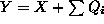. Similarly for .
Finally, a dynamic influence such as ) expresses the fact that if there are no other countervailing influences, a positive value of X causes an increase of Y. Direct influences are equivalent to algebraic influences on the derivative of the influenced variable (i.e., ).
A model fragment may assert other kinds of information besides influences: inequalities between quantities and numerical magnitudes, QSIM constraints or structural relationships.

3.21

SQPC smoothly integrates symbolic with numeric information, and is able to provide useful results even when only part of the knowledge is numerically bounded. The domain model includes symbolic or numeric magnitudes (both representing specific real numbers, known with uncertainty; numeric magnitudes constrain such numbers to lie within given ranges), dimensional information (what does the quantity represent: money, money/time, amounts, people, etc.), envelope schemas (stating the conditions under which a specific monotonic function over a tuple of variables is bounded by a pair of numeric functions) and tabular functions (numeric functions defined automatically by interpolating multi-dimensional data tables). The specific system or situation being modeled is described by the scenario definition, which lists objects that are of interest, some of the initial conditions, relations that hold throughout the scenario, and possibly time-varying boundary conditions on exogenous variables.

3.22

SQPC employs a hybrid architecture in which the model building portion is separated from the simulator. The domain model and scenario induce a set of logical axioms. SQPC uses these logical axioms to infer the set of model fragment instances that apply during the time covered by the axioms (called the active model fragments). Inferences performed by SQPC include those concerning structural relationships between objects declared in the scenario, and those aiming at computing the transitive closure of order relationships between quantities. A complete set of model fragment instances defines an initial value problem which is given to the simulator in terms of equations and initial conditions. If any of the predicted behaviors cross the boundaries of the current model the process is repeated: a new set of axioms is constructed to describe the system as it crosses the boundaries of the current model, another complete set of active model fragments is determined, and another simulation takes place.

3.23

Recently, SQPC has been extended with the capability of simulating non-autonomous systems, where the environment may affect the simulated system through time-varying exogenous variables (Brajnik, 1995). Furthermore, using an appropriate language based on temporal logic, the user can specify in the scenario description other kinds of behavioral constraints, to focus the simulation (Brajnik and Clancy, 1996a, Brajnik and Clancy, 1996b, Brajnik and Clancy, 1998).

3.24

SQPC is proven to construct all possible sequences of initial value problems that are entailed by the domain model and scenario; thanks to QSIM correctness, it produces also all possible trajectories.

The Authority's Problem

4.1

Let's return now to the problem mentioned in the introduction and use it as a case study.

4.2

Consider a central authority which has been charged with maintaining the quality of life for the N members of its society within certain limits. Quality of life for this problem is a function of two variables, per capita consumption -- measured in gross domestic product (GDP/N) -- and an index of environmental quality -- measured by pollution in parts per million (PPM) volume of atmospheric carbon dioxide, CO

being the largest contributor to green house gases. The authority may use any allocation scheme for assigning unconsumed national income (capital resources) to those types of investments pertinent to the task: increase capacity for producing consumer goods, given current technology; spend on R&D to reduce unit emissions in the production technology; increase capacity for abatement activity (in particular, land use policies); augment family planning services and education aimed at reducing the proportional growth rate of the population.

4.3

The structure -- objective/ state variables/ control variables -- is parallel to the optimization problem, but the goal is guidance and the relations between state and control variables are semi-quantitative.

4.4

For the moment we assume a constant population and a constant unit emissions coefficient. This case gives three policy instruments with which to guide the economy: two types of capital investment (consumer goods production, abatement) plus the allocation between current consumption and total investment. The latter refers to the accounting identity by which national income is either spent on current consumption or is saved and invested (increasing future consumption capacity).

4.5

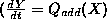
The basic model is:

where is the change per time period in the stock of emissions E (ppm/time), is the production function (GDP/time), A is a constant emissions coefficient (ppm/unit of GDP), is net emissions abated (ppm/time). In equation (1) we make the assumption that all changes per time period in the stock of emissions are due to anthropogenic activity except for a natural proportional decay factor m. We have implicitly assumed that all sinks for CO are full and we have not considered fertilization feedback effects (for a full discussion see (Wigley, 1993)). The production function depends on capital allocated to industrial production, is a function of capital allocated to the abatement sector. We assume that and are monotonically increasing functions. The second equation derives from the accounting identity of national income. Total investment (GDP/time), that is, the change per time in total capital, is what remains of national income after C (GDP/time) is allocated to current consumption.

4.6

The objective for the national authority is to invest in the various activities in such a way as to ensure members of the economy a high quality of life over time, by keeping consumption and environmental index within acceptable ranges. One way to understand how to achieve such an objective is to formulate certain relationships between variables of the model and explore their consequences. The initial decision is the choice between consumption and total investment (cfr. equation 2). We begin with a simple assumption: that total investment is constant and positive, meaning that the society is consuming less than it is producing

4.7

The next decision is how to allocate investment (cfr. equation 3) between that used for consumers goods production (

) and that used for abatement (

). We choose a second simple rule: invest an amount which is monotonically increasing with respect to the total stock of emissions and numerically bounded by a pair of increasing linear functions²

4.8

Finally, a lower bound is established for investment in production in order to keep up future consumption levels

4.9

Acceptable trajectories are defined as those for which per capita consumption does not decline below the original value and emission levels do not reach boundary values. The authority plans production so as to balance emissions with the system's natural and anthropogenic capacity to abate emissions and thereby guides the ecological system away from collapse and the economic system away from low levels of per capita consumption. That is, the authority's dynamic program for production must also be sustainable.

An Example

5.1

In this section we illustrate how the problem discussed above can be formulated and solved using SQPC. The idea is to use SQPC's language to define a model of the domain that can be reused to analyze different scenarios. These scenarios will be explored to understand the effects of the different rules mentioned above.

Domain Model

5.2

Three steps need to be carried out in order to define a domain model. First, the domain has to be conceptualized, that is entities and relationships that will play some role in the definition of scenarios have to be made explicit. The objective of such a step is to set a basis upon which to define, case by case, the specific system being analyzed as a set of interrelated instances of object types. By declaring entities in the scenario, or by adding or removing relationships between them, different scenarios can be defined. Second, types of quantities that are deemed useful need to be defined. Instances of these types of quantities will be then automatically become attributes of specific instances of objects and will be included in models for the simulation. Third, model fragments describing relevant and modular pieces of equations among quantities of objects need to be defined.

5.3

In our specific case, the taxonomy of the domain model consists of objects and relationships like societies, that are embedded within natural environments, that support a population of individuals who are involved in socio-economic activities like industrial production, pollution abatement and so forth. Figure 2 shows some entities and relationships included in the domain model.

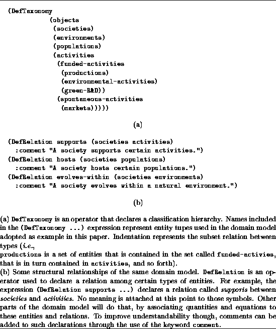
Figure 2: Portion of the taxonomy of the domain model

5.4

Several quantity types are then defined that characterize our perspective on this domain, shown in fig. 3.

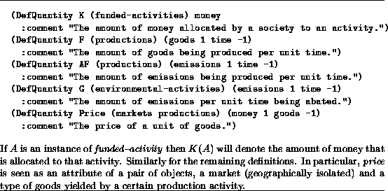
Figure 3: The definition of some quantity types

5.5

At this point we can define model fragments. For example, a model fragment might assert that for a society that supports a production activity, and that evolves within an environment, then the amount of emissions being released into the environment is positively influenced by the amount of goods being produced and that emissions accumulate over time to give the total amount of pollution present in the environment.

5.6

Figure 4 shows how these properties can be described. Several other model fragments, not shown here, are encompassed by the domain model that we use in this example.

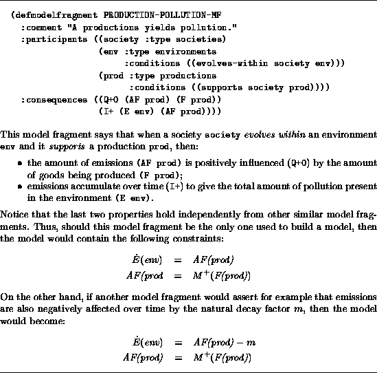
Figure 4: A compositional model fragment

Scenario And Resulting Simulations

5.7

The aim of the analysis is to evaluate the effects of previously discussed rules of thumb and explore their variations. The example centers on a situation in which there is a society (called world) evolving in an environment (earth). The society hosts a population (humans), it supports an industrial production called (timber-prod) and one kind of pollution abatement (smoke-filtering). A simple market exists for timber that determines the price for this product.

5.8

The situation is given to SQPC in terms of a scenario description which includes these entities, their relationships, initial conditions for some quantity, envelopes, and information about estimated changes in some of the quantities. Figure 5 provides additional details.

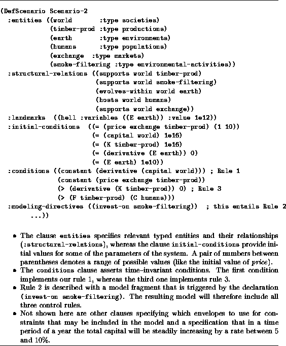
Figure 5: Part of the scenario definition

5.9

The information specified in this scenario description is given to SQPC that first decides which model fragments and envelopes are applicable to this situation. Then it constructs a qualitative model enriched with appropriate ranges and applicable envelopes. Finally SQPC defines all the possible initial states that are consistent with the conditions given in the scenario description and simulates the model until the defined horizon is reached (in this case a year).

5.10

The objective of the authority is to keep the economic society on a bounded path, but more specifically, it will try to avoid consumer rebellion (per capita consumption declines) and environmental hell (emissions hit an upper limit representing biosphere collapse). A possible scenario could include Rules 1 and 2 only. No government would adopt, however, such a set of rules: per capita consumption would decline at some point for all trajectories. Our scenario (figure 5) includes instead also Rule 3 and a relatively small value for

and

. Simulation of this scenario up to the end of the time period of interest (i.e., after one year) produces 9 behaviors (one of which is shown in figure 6). A common property of all such behaviors is that the per capita consumption will necessarily increase (i.e., no rebellion will take place). On the other hand, both a steady state in environmental hell and increasing emissions beyond environmental hell are plausible trajectories for the environmental index (like the behavior shown in figure 6). To avoid this, the rational step is for the decision-maker to increase investment in the abatement sector by varying

and

in Rule 2. Exploration of another scenario, that is similar to the one presented above (5) but that features a larger value of

and

, shows that emissions decline in all the 4 predicted behaviors, while maintaining an increasing per capita consumption. Therefore, thanks to SQPC soundness, the policy-maker is guaranteed that the last scenario, given the domain model, entails only sustainable-solutions.

5.11

Even in this very simple case, the advantages of using tools like SQPC are that within a single domain model several different simulations can be carried out quite easily, without requiring the user to define complex executable models. Furthermore, even with very weak quantitative information about functional relationships included in the model certain kind of conclusions can be drawn. Finally, thanks to the guaranteed coverage of the predicted solutions, the user of SQPC knows that the predicted behaviors includes all the possible trajectories of systems that are consistent with the given description.

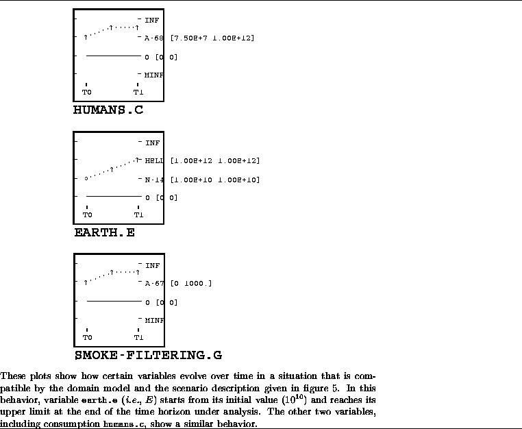
Figure 6: Plot of some variable for one of the predicted behaviors

Related Work

6.1: Within the Artificial Intelligence field there are several research directions that focus on socio-economic problems. Farley and Lin (Farley and Lin, 1990, Lin and Farley, 1991) focus on qualitative models of markets. They formulate economic theories (namely the law of demand and supply) in terms of markets that give rise to stable dynamics. That is, they see markets as homeostatic entities that support a dynamic equilibrium. Markets are then used as building blocks for more complex multi-market models, where interactions between markets are represented and considered. For example, to explore how a product market (representing income, investment and saving) may interact with a money market (income and investment). Markets are represented via purely qualitative relationships between variables. Comparative statics methods are then used to determine the effects of disequilibrium states on multiple interacting markets. The simulation methods adopted are less general than the ones we propose to use in this paper and in particular a simplifying assumption is made that certain feedback loops are negligible, enabling a stable trajectory to be followed. The approach we presented in this paper is equation-based (in the sense that there is no such thing as a predefined building-block like the market) and therefore is more general. In addition, we provide means for automatically assembling, on demand, an executable model from a library of fragments of equations and for integrating in a smooth way quantitative knowledge that may be available. Furthermore, recently developed methods for specifying trajectory constraints (like time-varying inputs or boundary condition problems) (Brajnik and Clancy, 1996a, Brajnik and Clancy, 1998) can be easily integrated into the architecture of SQPC, increasing in this way the expressiveness of the approach and supporting a wider spectrum of analyzes.
6.2: In the framework of the global-warming problem, probabilistic representations have been proposed. Distributions are given for parameter values in (Hope et al., 1993, Dowlatabadi and Morgan, 1993) while a fuzzy decision model is used in (Leimbach, 1996).
6.3: The area of economic theory which has received most attention from the AI perspective is the theory of choice, and in particular, reasoning and rational choice, learning behavior, and adaptive economic behavior (see e.g., Moss and Rae, 1992). Essentially this approach assumes that the information set available, or obtainable, by the decision-maker is so large that it is either impossible or uneconomical to calculate the constrained optimization solution. This issue is related to the existence of sufficient computational capacity for resolving complex problems. If the economic agent is unable to process the information it may resort to bounded rationality, or procedural rationality. Moreover, if the decision maker is in a disequilibrium situation, it may profit from experience, learn and adapt. This characterization of economic agent as having limited computational capacity but the ability to learn will be an interesting field to watch as it comes to influence mainstream economic research.
6.4: Another approach is that of artificial economies, wherein agents with varying characteristics are allowed to act and be acted upon. This provides a much more convincing economy than the usual one-agent or n-similar agents assumption (for examples, see (Lane, 1993) and (Bak et al., 1994)). An interesting project is currently being studied by a group associated with the Santa Fe Institute who are building a virtual stock market of around 100 agents who learn and adapt by detecting patterns in price movements arising from their trading (Stites, 1994).
6.5: Expert systems have also been used in theoretical economics, see (Artis et al., 1992) who argue that macro econometric models can be improved by incorporating experts' intuitive prediction rules into the models.

Future Work And Conclusions

7.1: These preliminary results provide an indication of how a set of rules of thumb can be validated by the decision maker using a qualitative simulator, and an indication of the type of information available for time paths of relevant variables. They show that even with very poorly specified knowledge of models or scenarios certain useful questions can be posed and answered.
7.2: This should be a better base from which to make policy recommendations for the systems with complicated trade-offs which are inherent to the analysis of economic growth and environmental quality. Moreover, these techniques make the maximum use of the qualitative information that is available in economic theory. They also force the theorist to formalize rules of thumb (i.e.,
specific policies/control laws) for allocating between resources since optimization is no longer available. We think that the use of such tools by students and policy-makers could serve to deepen their understanding and intuitive awareness of the complexity of dynamic allocation decision problems. For the problem at hand, direct experience with game-like simulations could greatly increase sensitivity to the delicate and controversial questions which underlie the real world allocation problem.
7.3: Future work will aim at introducing a further policy option for the authority to deal with emissions -- investment in research and development to reduce the technology coefficient (emissions per output). We also intend to introduce demographic models of population dynamics, which greatly complicates the time path for the per capita consumption. Then yet another policy option will be available -- investment in a sector which provides health, family planning and educational services, under the hypothesis that such investment reduces the natural growth rate of the population.

Acknowledgements

The simulations discussed and shown in the paper have been performed using SQPC, a program developed by one of the authors. SQPC in turns is based upon QSIM, a qualitative simulation system developed by the Qualitative Reasoning Group at the Artificial Intelligence Laboratory, The University of Texas at Austin led by prof. Ben Kuipers.

QSIM and other results of the Qualitative Reasoning Group are accessible by World-Wide Web via <http://www.cs.utexas.edu/users/qr>.

A special thanks goes to Bert Kay, who was tragically killed in Palo Alto on June 12, 1997.

Notes

¹: An extemal differential equation is automatically obtained from a qualitative differential equation enriched with envelopes and gives upper and lower bounds for each state variable. See (Kay, 1996a) for details.
²: The fact that bounding functions are linear should not lead to the conclusion that the bounded functions should include only linear functions.

References

Artis et al., 1992: M. Artis, S. Moss, and P. Ormerod. The development of intelligent macroeconometric models and modelling procedures. In Moss and Rae, 1992, pages 167-176.
Bak et al., 1994: P. Bak, K. Chen, J. Scheinkman, and M. Woodford. Aggregate fluctuations from independent sectoral shocks: self-organized criticality in a model of production and inventory dynamics. Richerche Economiche, 47:3-30, 1994.
Berleant and Kuipers, 1988: D. Berleant and B.J. Kuipers. Using incomplete quantitative knowledge in qualitative reasoning. In Proc. of the Sixth National Conference on Artificial Intelligence, pages 324-329, 1988.
Brajnik and Clancy, 1996a: G. Brajnik and D. J. Clancy. Temporal constraints on trajectories in qualitative simulation. In B. Clancey and D. Weld, editors, Proc. of the Tenth National Conference on Artificial Intelligence, pages 979-984. AAAI Press, Aug. 1996.
Brajnik and Clancy, 1996b: G. Brajnik and D. J. Clancy. Temporal constraints on trajectories in qualitative simulation. In Working papers of the Tenth International Workshop for Qualitative Reasoning, pages 22-31, Fallen Leaf Lake, CA, May 1996. AAAI Technical Report WS-96-01.
Brajnik and Clancy, 1998: G. Brajnik and D. J. Clancy. Focusing qualitative simulation using temporal logic: theoretical foundations. Annals of Mathematics and Artificial Intelligence, 1998. To appear.
Brajnik, 1995: G. Brajnik. Introducing boundary conditions in semi-quantitative simulation. In Ninth International Workshop on Qualitative Reasoning, pages 22-31, Amsterdam, May 1995.
Dowlatabadi and Morgan, 1993: H. Dowlatabadi and M.G. Morgan. A model framework for integrated studies of the climate problem. Energy Policy, 21:209-221, 1993.
Falkenhainer and Forbus, 1991: B. Falkenhainer and K. Forbus. Compositional modeling: finding the right model for the job. Artificial Intelligence, 51:95-143, 1991.
Faltings and Struss, 1992: B. Faltings and P. Struss. Recent advances in qualitative physics. MIT Press, 1992.
Farley and Lin, 1990: A. M. Farley and K. P. Lin. Qualitative reasoning in economics. Journal of Economic Dynamics and Control, 14:465-490, 1990. North-Holland.
Farquhar and Brajnik, 1994: A. Farquhar and G. Brajnik. A semi-quantitative physics compiler. In 8th International Workshop on Qualitative Reasoning about physical systems, pages 81-89, Nara, Japan, 1994.
Farquhar, 1994: A. Farquhar. A qualitative physics compiler. In Proc. of the 12th National Conference on Artificial Intelligence, pages 1168-1174. AAAI Press / The MIT Press, 1994.
Hope et al., 1993: C. Hope, J. Anderson, and P. Wenman. Policy analysis of the greenhouse effect. Energy Policy, 21:327-338, 1993.
Iwasaki and Low, 1991: Y. Iwasaki and C. M. Low. Model generation and simulation of device behavior with continuous and discrete changes. Technical Report KSL 91-69, Knowledge Systems Laboratory -- Stanford University, November 1991.
Kay and Kuipers, 1993: H. Kay and B.J. Kuipers. Numerical behavior envelopes for qualitative models. In Proc. of the Eleventh National Conference on Artificial Intelligence. AAAI Press/MIT Press, 1993.
Kay, 1996a: H. Kay. Refining Imprecise Models and Their Behaviors. PhD thesis, Department of Computer Sciences, The University of Texas at Austin, Dec 1996.
Kay, 1996b: H. Kay. SQsim: a simulator for imprecise ODE models. TR AI96-247, University of Texas Artificial Intelligence Laboratory, March 1996.
Kay, 1997: H. Kay. Robust identification using semiquantitative methods. In IFAC Symposium on Fault Detection, Supervision and Safety for Technical Processes (SAFEPROCESS'97), Hull, UK, Aug 1997.
Kuipers, 1994: B.J. Kuipers. Qualitative Reasoning: modeling and simulation with incomplete knowledge. MIT Press, Cambridge, Massachusetts, 1994.
Lane, 1993: D. Lane. Artificial worlds and economics, part II. Journal of Evolutionaly Economics, 3:177-197, 1993.
Leimbach, 1996: M. Leimbach. Development of a fuzzy optimization model, supporting global warming decision-making. Environmental and Resource Economics, 7:163-192, 1996.
Lin and Farley, 1991: K. P. Lin and A. M. Farley. Qualitative economic reasoning: a disequilibrium perspective. Computer Science in Economics and Management, 4:117-133, 1991.
Moss and Rae, 1992: S. Moss and J. Rae. Artificial Intelligence and Economic Analysis. Edward Elgar, Hants, UK, 1992.
Sebenius, 1984: J. K. Sebenius. Negotiating the Law of the Sea. Harvard University Press, Cambridge, 1984.
Siebert, 1987: H. Siebert. Economics of the Environment. Springer-Verlag, Berlin, 1987.
Stites, 1994: J. Stites. W. Brian Arthur. The Bulletin of the Santa Fe Institute, Winter:5-8, 1994.
Wigley, 1993: T.M.L. Wigley. Balancing the carbon budget. implications for projections of future carbon dioxide concentration changes. Tellus, 45(B):409-425, 1993.

Button Return to Contents of this issue