©Copyright JASSS

JASSS logo ----

Jill Bigley Dunham (2005)

An Agent-Based Spatially Explicit Epidemiological Model in MASON

Journal of Artificial Societies and Social Simulation vol. 9, no. 1
<https://www.jasss.org/9/1/3.html>

For information about citing this article, click here

Received: 02-Feb-2005    Accepted: 15-Dec-2005    Published: 31-Jan-2005

PDF version


* Abstract

This paper outlines the design and implementation of an agent-based epidemiological simulation system. The system was implemented in the MASON toolkit, a set of Java-based agent-simulation libraries. This epidemiological simulation system is robust and extensible for multiple applications, including classroom demonstrations of many types of epidemics and detailed numerical experimentation on a particular disease. The application has been made available as an applet on the MASON web site, and as source code on the author's web site.

Keywords:
Epidemiology, Social Networks, Agent-Based Simulation, MASON Toolkit

* Introduction

Objective

1.1
There are many simulation toolkits available, requiring various levels of programming experience. One of these, the MASON toolkit, is a set of Java libraries for agent-based modeling (ABM). MASON is quite user-friendly, and many programmers already have experience with Java, but can all the required elements of a realistic epidemiology model be implemented in MASON?

1.2
This paper outlines the design and implementation of an agent-based, spatially explicit simulation for the study of infectious disease in a human population. The simulation is readily extensible for multiple applications within this area, and thus can be a good starting point for other researchers. It also demonstrates that the MASON libraries are sufficient to create a realistic, extensible system that is also easy to use for demonstration purposes. The system has enough flexibility to model epidemics with many different parameters in a demonstration setting. However, the parameters offer enough detail to be useful for focused numerical experimentation. It is the author's hope that interested researchers will take this code, extend and modify it, and use it for their own research.

Background

1.3
Epidemics have been modeled mathematically for over a century. From Louis Pasteur's work on cholera epidemics, a system of partial differential equations was developed which modeled the change in percentage of a population over time (Wasserman and Faust 1994). From this early model, we get the standard categories used to describe an epidemic. The SIS (Susceptible-Infected- Susceptible) model represents diseases for which there is no acquired immunity; once a person has been infected and recovers, he or she is susceptible to the disease once again. In the SIR (Susceptible-Infected-Removed) model, an individual passes from susceptible to infected to removed (the euphemistic "removed" includes both those with immunity and those that are dead). A more realistic SEIR or SLIR (Susceptible-Exposed/Latent-Infected-Removed) model adds an intermediate step which represents the latent period between exposure and external symptoms and thus can take into account differing degrees of infectiousness which occur during these two stages (Deiekmann and Heesterbeek 2000). Figure 1 shows a visual representation of the various stages used.

Figure 1
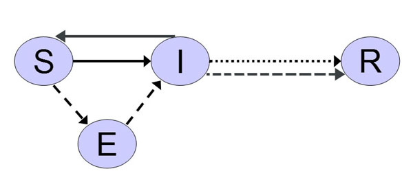
Figure 1. A flowchart of possible states in an epidemic model

1.4
More recently, other types of epidemic models have been explored: subpopulation models, spatial models and social network models. Subpopulation models attempt to address the implicit assumption of full, homogenous mixing that is part of the differential equations model. Spatial models address the non-spatial character of the old models. Social network models differentiate between individuals, especially in the case of sexually transmitted diseases (Bian 2004).
Other Work

1.5
The use of network-based models in epidemiology has become an active topic in the scientific literature. Current simulation work has incorporated a variety of techniques, including agent-based modeling and cellular automata, into network simulations. Groups such as the Center for Discrete Mathematics and Theoretical Computer Science (DIMACS) at Rutgers University have begun to focus on the possibilities in this subject (DIMACS 2004). At the University of North Texas, Sangeeta Venkatachalam and Armin Mikler have created a simulation using cellular automata, modified to accommodate spatial interactions (Venkatachalam and Mikler 2005).

1.6
Joshua Epstein and others from the Brookings Institute's Center on Social and Economic Dynamics have developed agent-based simulations using their in-house Java API, Ascape, and other tools. Their purpose is to study vaccination and containment strategies in the event of bioterrorist attack involving smallpox or other infectious diseases (Epstein, Cummings et al. 2002).

1.7
Catherine Dibble, Assistant Professor of Geography at the University of Maryland, has developed simulations using the GeoGraphs agent-based computational laboratory built upon RePast. Her research team developed GeoGraphs to "conduct theory-driven explorations of distributed dynamic processes on richly-structured landscapes" (Dibble 2004). Specifically she has been exploring agent-based epidemiological models using GeoGraphs along with genetic algorithms to explore parameter space. Her simulations incorporate realistic geographic landscapes as well as small-world and scale-free networks (Dibble and Feldman 2004).

1.8
Richard Crandall, the director of the Center for Advanced Computation at Reed College, and his students have developed a simulation system called Conflagrator to study epidemics with nonlinear techniques in both continuum and discrete models. Along with members of the Oregon Bioterror Taskforce, the Reed group has been carrying out research on epidemics and exploring preferential vaccination strategies. He and his students have been exploring ways to combine cellular automata models with interaction networks (Dworkin 2004).
Simulation Framework

1.9
Ling Bian proposed a simulation framework which addresses four major assumptions implicit in the classical differential equations model. Bian's framework is based on the following assumptions: individuals are different; individuals interact locally; individuals are mobile; and the interactions are heterogeneous. Her framework combines agent-based modeling with homogenous interaction networks over a spatial domain (Bian 2004) and is similar to the work being done by Epstein, Dibble, and others. However, other types of models mentioned earlier (subpopulation, social network, simple spatial models, etc) have addressed some of these assumptions, but never all at one time.

1.10
Heterogeneous interactions are demonstrated in Bian's paper through a two-layered interaction network. One layer consists of homes and the other layer of workplaces. Contact structures and intimacy of contact differ between the two layers, which is an important insight from her paper. Humans have somewhat predictable interactions which can be modeled in this way. Figure 2, taken from Bian's paper, illustrates this two-layered network.

Figure 2
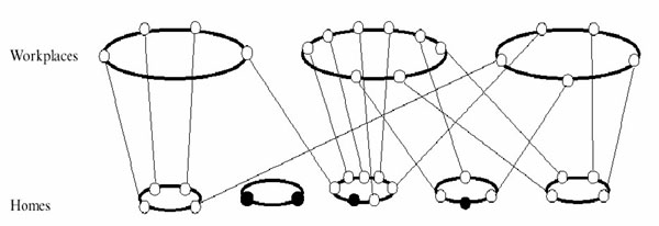
Figure 2. Two-layered network (Bian 2004)

The MASON Toolkit

1.11
The MASON toolkit is a set of libraries in Java, developed to support discrete multiagent simulations. MASON was developed at George Mason University as a joint effort of the Evolutionary Computation Laboratory and the Center for Social Complexity (Luke, Cioffi-Revilla et al. 2004). A feature of MASON which influenced the decision to use it for this project is its ability to decouple the simulation from real-time visualization, which makes running long batches of simulations much faster. MASON has no graphical capabilities built in, but output files can be created in formats easy to import into third-party analysis packages.

* System Implementation

Java Classes and Agent Types

2.1
The author implemented this simulation system with five Java classes: The Human agent class handles the various behaviors and biological processes of the humans being modeled. In this version of the simulation, it includes physical movement between home and work, decision-making with regard to taking sick days, and simplified biological processes involved in the infection.

2.2
The agent class could be extended to create derived agents other than the human agents. Animal agents might share biological processes and some movement rules with humans, while another type of agent (such as a plant) would have biological processes but no movement rules. An inanimate object might also be modeled as an agent in some cases. For example, in simulating a disease which spreads through fomites, contaminated linens and other items might be modeled as agents, with rules to govern the rate of decrease in infectiousness.

Figure 3
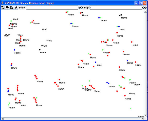
Figure 3. Simulation display window. Susceptible agents are shown in green, exposed in blue, infected in red, and removed in black

Parameters

2.3
This simulation has several parameters that the user can vary. For example, NUM_INFECTED, NUM_REMOVED, and NUM_EXPOSED control the initial number of humans in each of these states. A combination of the NUM_HUMANS parameter with the four display size parameters can be used to set up a specific population density for the simulation. A detailed description of the simulation parameters is shown in the following three tables. Table 1 displays the parameters for the landscape and population of the simulation and their default values. The default values were chosen so that a first-time user can see a simple, understandable demonstration.

Table 1: Basic simulation parameters

ParameterDefault ValueDescription
XMIN 0Controls display size and shape
XMAX800Controls display size and shape
YMIN 0Controls display size and shape
YMAX600Controls display size and shape
DIAMETER 8Physical size of agents
NUM_HUMANS40Total humans in simulation
NUM_INFECTED 5Number of humans initially infected
NUM_REMOVED 0Number of humans initially removed
NUM_EXPOSED 0Number of humans initially exposed
DAY_LENGTH500Number of time steps per simulation day

2.4
A second set of parameters is specific to the disease being modeled. Users can choose the type of model (SIS, SIR, SEIS, or SEIR epidemic), the infection distance, length of exposed and infection periods, and infectivity rates for both the exposed and infected states (parameters referring to exposed periods are ignored when the simulation has no exposed period). Parameters whose names end in "DAYS" are then divided by the DAY_LENGTH parameter to obtain per-time-step values used in calculations.

2.5
Infected and exposed periods can be set in two ways: a constant length, or a length drawn from a distribution. The constant-length version is set by setting the MIN, MAX, and MEAN variables to the same values. When the MIN and MAX parameters are not equal, the lengths are drawn from a truncated normal distribution with given MEAN parameter. These parameters are outlined in Table 2.

Table 2: Disease-specific simulation parameters

ParameterDefault ValueDescription
SIR_MODEL TrueFlag to indicate inclusion of removed state.
SEIR_MODEL FalseFlag to indicate inclusion of exposed/latent state.
INFECTION_DISTANCE20Radius of infectiousness
MEAN_INFECTED_TIME_DAYS1.0
MAX_INFECTED_TIME_DAYS1.0
MIN_INFECTED_TIME_DAYS1.0
MEAN_EXPOSED_TIME_DAYS1.0
MAX_EXPOSED_TIME_DAYS1.0
MIN_EXPOSED_TIME_DAYS1.0
INFECTIVITY_RATE_EXPOSED_DAYS0.75
INFECTIVITY_RATE_DAYS0.5

2.6
The final parameters are societal and personal parameters (Table 3). A variable representing personal health is calculated for each human at simulation start, which is drawn from a modified normal distribution (mean 0.5, standard deviation 0.5, with values truncated to the range [0, 1]. 0 indicates severe immunodeficiency.) Health affects both the likelihood of infection as well as infection duration when variable infection lengths are being modeled. Another parameter which affects human agent behaviors is the Acceptance parameter, which reflects how likely individuals are to accept that they are sick and stay home from work; the parameter is shared by all human agents. Mean and standard deviation of home and workplace sizes are also society-wide parameters, which should be updated depending on the society being modeled. By default, home size and standard deviation are based on US Census Bureau (2000) statistics. Default workplace mean size and standard deviation, however, are based on best guesses, as relevant statistics were not as readily available.

Table 3: Societal and personal simulation parameters

ParameterDefault ValueDescription
health_factorBetween 0 and 1Index of a human''s general health
ACCEPTANCE0.5Likelihood of taking a sick day when ill
HOME_MEAN 2.59Mean home size
HOME_SD 1.42Standard deviation of home size
WORK_MEAN 10Mean workplace size
WORK_SD 3.5Standard deviation of workplace size

Input

2.7
There are two methods which can be used to input simulation parameters: via the console and via input files. Additionally, default values for each parameter are automatically loaded when the simulation is started without a specified input file.

2.8
The simulation console, which is only visible when the simulation is run in GUI mode, shows a set of modifiable parameters under the "mode" tab. In GUI mode, the parameters are slightly simplified to facilitate demonstration. Figure 4 displays these parameters. In addition, individual agents can also have their status (infected, removed, etc.) changed on the fly using the display console.

Figure 4
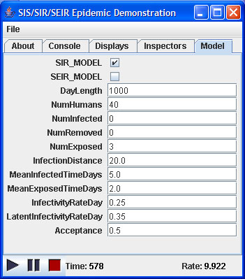
Figure 4. The simulation console

Alternatively, simulation parameters can be specified using an input file. Using the input file allows control over the full set of parameters, including setting maximum and minimum exposed and infection lengths to allow variable lengths for these phases. Home and workplace size distributions can also be varied using input files.

Output

2.9
Output is captured in the form of aggregate statistics: the number of individuals in each of the possible states (S, E, I or R) at every nth time step. This information is written to a comma-delimited text file. This format is viewable with a standard text editor and readable by humans, and is interpretable by spreadsheet and database programs such as Microsoft Excel and Access. Because MASON does not have any graphing or output processing capabilities built in, this simple file format is ideal for use with third-party analysis packages. The design of the simulation makes it easy to modify the format of the output files as needed.

Initialization

2.10
When the simulation starts, the first step is to apply the parameters to set up its agents and locations. First, the environment is created. This simply means setting up the simulation area based on the four display size parameters from table 1.

2.11
Next, the human agents are created, and health factors for each agent are generated according to a normal distribution, as discussed above. Agents are chosen at random to fill the required numbers of initially infected, exposed, and removed agents specified. All other agents are initially set as susceptible to infection. The agents are initially placed randomly across the landscape.

2.12
Then the locations are created and humans are each assigned to a home and a workplace. Sizes of each home and workplace are drawn from a normal distribution, which can be modified to mirror various home and workplace size distributions. Homes are placed randomly across the simulation area, while workplaces are confined to the top left quadrant to approximate an "urban center". Now the simulation is ready for the scheduler to take over. The scheduler steps the simulation through time, allowing any agents to perform their tasks.

Agent Rules

2.13
The humans in this simulation lead fairly humdrum lives: they travel between work and home. Epoch in this simulation can be thought of as 8 AM. At this moment, all humans begin traveling toward their assigned workplaces. Once they get sufficiently close to their work locations, the human agents each start an internal timer. When an individual human's timer reaches 1/3 of the day length, it leaves work and travels home. Agents have variable distances to travel, and so arrive at (and leave) work at staggered times.

2.14
The human agents move in a straight line toward their target location (home or work, depending on time of day) at a constant speed based on distance to target. The day length parameter is also taken into account, so that an agent in a simulation with a fine time-scale will spend the same proportion of the day traveling the same distance as an agent in a temporally coarser-grained simulation. The velocity at which the agents move can be adjusted in the code.

2.15
As mentioned in the initialization section, the agents are initially placed over the landscape at random. However, as the agents' routines of commuting to and from work are established, the agents travel relatively regular paths.

2.16
If a human is infected (symptomatic) at epoch, that agent must decide whether to take a sick day and stay home from work. A random Boolean generator is employed as a coin flip weighted by the simulation's Acceptance parameter. Figure 5 outlines these simple behaviors.

Figure 5
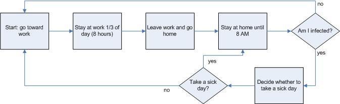
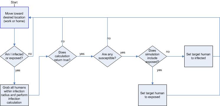
Figure 5. Human behavior rules

2.17
The rules for Human behavior in this simulation include rules, which govern the unconscious biological process of disease spread. If an infectious agent (whether in the exposed or infected states) passes within the INFECTION_DISTANCE of a susceptible agent, a calculation is performed to determine if that agent will become infected (or exposed, in the case of an SEIR or SEIS simulation). This process is summarized in Figure 6. While most infections will be passed while the agents are at their home or work locations, the agents also come in contact during their "commutes" between the two locations and can pass the infection at that time. This approximates the shorter contacts humans in society have while riding public transportation, buying a cup of coffee and a newspaper, or picking up groceries on the way home. Timers, which can be set to variable latent and infected lengths chosen from a distribution, keep track of when an individual human will move on to the next state. Figure 7 shows an agent's progression through the epidemiological phases.

Figure 6
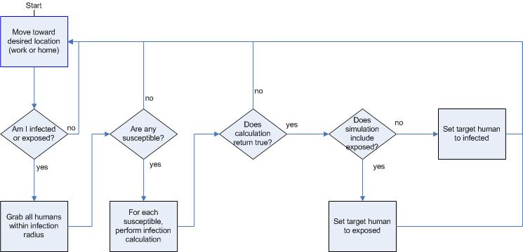
Figure 6. Infection behaviors

Figure 7
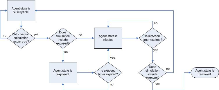
Figure 7. Movement through the infection phases

* Example Runs

3.1
To demonstrate the simulation system, three sets of sample runs, representing influenza, RSV and Lassa, have been completed and averaged over 20 runs. Influenza was chosen because of its prevalence and recent concerns over vaccine shortage and new recombinant strains. RSV was chosen because of three interesting characteristics: incomplete or nonexistent acquired immunity, prevalence among children, and lack of definite diagnosis in many cases. Lassa, a viral hemorrhagic fever, was chosen to show a completely different type of infection: an exotic disease that has been suggested as a biological weapon and certainly has the ability to induce terror in those familiar with its symptoms.

Influenza

3.2
Influenza (or "the flu") is a commonly known respiratory infection throughout the world. The flu is highly infectious and can be life-threatening to the elderly and those with chronic illness or immunodeficiency (Hawker, Begg et al. 2001). It is of great interest to health authorities almost every winter, and especially this past year because of a shortage of vaccines.

3.3
The first simulation provides a rough outline of a flu-like epidemic. Table 4 displays some of the parameter values used. To model this type of epidemic, the model was set up in SEIR mode. Realistic values for the range of exposed and infected times were used. A relatively high infection rate for both phases of the disease were used, while an acceptance value of 0.5 indicates that symptomatic individuals only have a 50% likelihood of staying home.

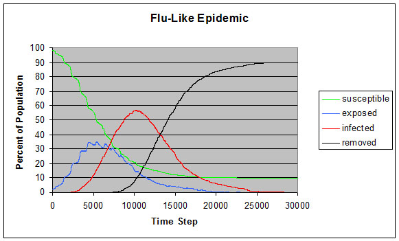
Table 4: Some parameters used for influenza-like epidemic demonstration

INFECTION_DISTANCE =20
DAY_LENGTH =1000
MEAN_INFECTED_TIME_DAYS=5.0
MAX_INFECTED_TIME_DAYS=6.0
MIN_INFECTED_TIME_DAYS=4.0
INFECTIVITY_RATE_DAYS=0.2f
MEAN_TIME_EXPOSED_DAYS=2.0
MAX_TIME_EXPOSED_DAYS=5.0
MIN_TIME_EXPOSED_DAYS=1.0
INFECTIVITY_RATE_EXPOSED_DAYS=0.3f
NUM_HUMANS =100
NUM_INFECTED =0
NUM_REMOVED =0
NUM_EXPOSED =2
ACCEPTANCE =0.5f
SIR_MODEL =1
SEIR_MODEL =1

3.4
The average of 20 runs with these parameters is displayed in figure 8. The epidemic has a steep infection curve, which dies down by about day 15, by which time, only 10% of the population has never been infected. This follows the same trends as a real influenza epidemic, although faster and more prevalent. Once the model has been properly parameterized, the infection curves could be compared and contrasted with other model types.

Figure 8
Figure 8. Flu-like epidemic

RSV

3.5
Respiratory syncytial virus (RSV) causes upper and lower respiratory infections. It can cause serious outbreaks, especially among children, the elderly, and the immunocompromised. However, most cases are not specifically diagnosed as RSV (Hawker, Begg et al. 2001). RSV infection leaves the individual with little or no immunity to future RSV infections, so it is best modeled as an SEIS epidemic.

3.6
Table 5 shows some of the parameters used in modeling this type of epidemic. Three states are allowed in this model: susceptible, exposed, and infected, after which the individual returns to the susceptible pool and may become infected again. Because of the acute character of RSV and its prevalence among children, the higher acceptance value of 0.7 was used here.

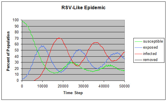
Table 5: Some parameters used for RSV-like epidemic demonstration

INFECTION_DISTANCE =20
DAY_LENGTH =1000
MEAN_INFECTED_TIME_DAYS=8.0
MAX_INFECTED_TIME_DAYS=10.0
MIN_INFECTED_TIME_DAYS=6.0
INFECTIVITY_RATE_DAYS=0.25f
MEAN_TIME_EXPOSED_DAYS=5.0
MAX_TIME_EXPOSED_DAYS=8.0
MIN_TIME_EXPOSED_DAYS=2.0
INFECTIVITY_RATE_EXPOSED_DAYS=0.25f
NUM_HUMANS =100
NUM_INFECTED =0
NUM_REMOVED =0
NUM_EXPOSED =2
ACCEPTANCE =0.7f
SIR_MODEL =0
SEIR_MODEL =1

3.7
Figure 9, the average over 20 simulations, shows the periodic character of a disease like RSV, although at a lower time scale and higher prevalence.

Figure 9
Figure 9. RSV-like epidemic

Lassa Virus

3.8
Lassa virus is a viral hemorrhagic fever, a severe infection with high mortality rate. The most famous of this type of infection is Ebola, the "flesh eating virus." This type of infection is uncommon outside of the endemic areas. For Lassa, this area is rural West Africa, where the virus is carried by rats (Hawker, Begg et al. 2001). However, Lassa and other hemorrhagic fevers have been suggested as possible biological weapons, and therefore are timely for study and simulation.

3.9
Lassa was modeled as an SEIR infection, and its parameters are shown in Table 6. One interesting change is in the infection distance parameter. Unlike respiratory infections, where coughing can spray an aerosol of infectious material, Lassa is usually transmitted by closer contact. After symptoms have emerged, transmission will also be lower, because the acuteness of the disease will be impossible to ignore. This also accounts for the maximum acceptance value of 1.0, meaning that once symptoms have emerged, the individual is unlikely to be moving around in public. The infectivity rate during the exposed period has been set to what is probably an unrealistically high value, but this can be explored upon further research.

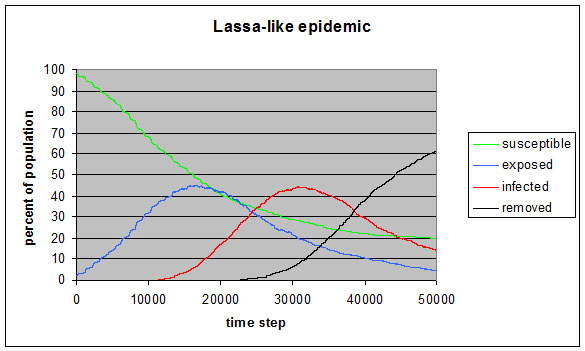
Table 6: Some parameters used for Lassa-like epidemic demonstration

INFECTION_DISTANCE =10
DAY_LENGTH =1000
MEAN_INFECTED_TIME_DAYS=10.0
MAX_INFECTED_TIME_DAYS=20.0
MIN_INFECTED_TIME_DAYS=5.0
INFECTIVITY_RATE_DAYS=0.15f
MEAN_TIME_EXPOSED_DAYS=10
MAX_TIME_EXPOSED_DAYS=21.0
MIN_TIME_EXPOSED_DAYS=6.0
INFECTIVITY_RATE_EXPOSED_DAYS=0.35f
NUM_HUMANS =100
NUM_INFECTED =0
NUM_REMOVED =0
NUM_EXPOSED =2
ACCEPTANCE =1.0f
SIR_MODEL =1
SEIR_MODEL =1

3.10
Figure 10 displays the average results over 20 runs with these parameters. This graph has a similar character to the influenza simulation shown in Figure 7, although this epidemic has a longer duration, only starting to settle down at the end of 50 days. This gives health officials more time to react to this epidemic and slow its spread. If a similar trend is preserved after further refinement, this may indicate that Lassa and other viral hemorrhagic fevers are not ideal biological weapons, despite their terrifying symptoms.

Figure 10
Figure 10. Lassa-like epidemic demonstration

* Infection Push vs. Infection Pull

4.1
In this simulation, infectious agents search for susceptible agents within a specified radius of their current position and "push" the infection onto the susceptible population with a certain probability. This is not an accurate representation of reality, but neither is the opposite situation: susceptible agents finding infectious agents within a radius and "pulling" the infection into themselves with a certain probability. However, for the purposes of this simulation, a reasonable method is needed to spread the infection. In the previous sample runs, an infection pushing algorithm was used. For comparison, the flu-like epidemic runs were repeated using the infection pulling algorithm. Figure 11 can be compared with Figure 8 to see that this produces comparable output.

Figure 11
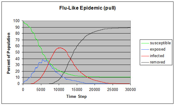
Figure 11. Flu-like epidemic using infection pull instead of push

* 5. Intervention Policies

5.1
Two unique aspects of this model are useful for demonstrating intervention policies. The first is the acceptance parameter, which gives the likelihood that an infected human will stay home instead of going to work when the next day begins. By varying this parameter, effects of closing schools and workplaces as well as the possible effects of a public service campaign ("Just Stay Home") can be studied.

5.2
The second unique feature is part of the MASON toolkit. When running the simulation in interactive mode (with visualization), individual agents can be selected, and their health status can be changed by toggling the checked boxes under the Inspectors tab on the console window. This can be used for a variety of interesting explorations, such as choosing on the fly which agents will be infected (a terrorist cell decides which of its agents is positioned to do the greatest damage if infected) or carefully determining which agents will be vaccinated (setting particular agents to Removed). Of course, random vaccination at varying coverage can also be studied by starting the simulation with some number of agents set as removed.

* 6. Conclusion

6.1
The simulation described in this paper has been implemented using the MASON multiagent toolkit. It has been demonstrated on 3 diverse diseases, and provides an excellent base for further investigation. The MASON toolkit was sufficient to implement a simulation with all the required elements, as described by Ling Bian (2004). While the results of the example runs are meant as demonstrations, the infection curves created are a qualitative match to real-world epidemic data. With proper parameterization, this model could be used for realistic simulations.

Future Work

6.2
This simulation is a flexible framework, which can be extended to accommodate many additional ideas and avenues of research. Ling Bian mentions some examples in her framework paper, including modeling weekend population interactions, incorporating realistic landscapes, and modeling vector-borne diseases such as those carried by rats and mosquitoes (Bian 2004). Non-human animals such as these could be implemented as a class which inherits from the general class Agents, with different behaviors from human agents.

6.3
While the example results presented in this paper have been simulated using the algorithm presented above (Figure 6) for determining when the infection will be passed, a change to the code allows for the R0 estimation proposed by (Lipsitch et al 2003): instead of determining the infection status of the individual, then using a stochastic coin flip to determine whether the infection will be passed to the susceptible agent, perform the stochastic step first, then determine whether the receiving agent is susceptible (see Figure 12.)

Figure 12
Figure 12. Revised infection flowchart

6.4
Groundbreaking research by Albert-Laszlo Barabasi indicates that the social network, the links between individuals in human society, is most likely a scale-free network, which is characterized by a very specific type of skewed distribution (Barabasi 2002). This type of network allows for specific emergent behavior which is not possible with other configurations, for example the emergence of superspreaders in a population. An easy extension to this simulation would be to implement functions to create other distributions such as the power-law distribution needed to create scale-free characteristics.

6.5
Another extension would also strengthen the support for network research. The author envisions adding an additional visualization window which would show the agents in a network layout, and would add links dynamically for agents which came within infection distance while traveling between locations. Tools for starting the simulation with a specified interaction network and for saving the network information created by the simulation would be highly useful future extensions. Varying the distributions used in different areas of the simulation would be a fruitful topic in social network research.

6.6
Further parameterization of the simulation for specific diseases is a vital next step before using the simulation to model a realistic epidemic. Once parameterization is complete, validation can proceed.

6.7
Other future enhancements include adding more personal characteristics and behaviors to differentiate individual humans and additional important environmental characteristics such as weather. For infections which can be passed through surface contacts and fomites, a fading trail of contamination could be implemented which follows infectious individuals. Each of these enhancements should be possible using the MASON toolkit.

* Acknowledgements

The author would like to thank the following people for their assistance: Keith Sullivan, Daniel Dunham, Liviu Panait, Dawn Parker, Catherine Dibble and Johan Bjursell.

* References

BARABASI, A.-L. (2002). Linked: The New Science of Networks. New York, Perseus Publishing.

BIAN, L. (2004). "A Conceptual Framework for an Individual-Based Spatially Explicit Epidemiological Model." Environment and Planning B: Planning and Design 31: 381-395.

US CENSUS BUREAU (2000). American Fact Finder.

DEIEKMANN, O. and J. A. P. Heesterbeek (2000). Mathematical Epidemiology of Infectious Disease: Model Building, Analysis, and Interpretation. New York, John Wiley & Sons, Inc.

DIBBLE, C. (2004). GeoGraph Models for Controlling Epidemics. School of Computational Sciences Research Colloquium. George Mason University.

DIBBLE, C. and P. G. Feldman (2004). "The GeoGraph 3D Computational Laboratory: Network and Terrain Landscapes for RePast." Journal of Artificial Societies and Social Simulation 7(1).

DIMACS (2004). Center for Discrete Mathematics and Theoretical Computer Science, Rutgers University.

DWORKIN, A. (2004). Mathematical supermodels refine epidemic predictions. The Oregonian. Portland, Oregon.

EPSTEIN, J., D. A. T. Cummings, et al. (2002). "Toward a Containment Strategy for Smallpox Bioterror: An Individual-Based Computational Approach." Brookings Institute Center on Social and Economic Dynamics Working Paper #31.

HAWKER, J., N. Begg, et al. (2001). Communicable Disease Control Handbook. Oxford, Blackwell Science Ltd.

LIPSITCH, Marc, Ted Cohen, et al. (2003). "Transmission Dynamics and Control of Severe Acute Respiratory Syndrome." Science 300:5627:1966-1970.

LUKE, S., C. Cioffi-Revilla, et al. (2004). MASON: A New Multi-Agent Simulation Toolkit. 2004 SwarmFest Workshop.

VENKATACHALAM, Sangeeta, Armin Mikler, A. R. (2005). Towards Computational Epidemiology : Using Stochastic Cellular Automata in modeling spread of diseases. Proceedings of the 4th Annual International Conference on Statistics, Mathematics and Related Fields, Honolulu, HI.

WASSERMAN, S. and K. Faust (1994). Social Network Analysis: Methods and Applications, Cambridge University Press.

----

ButtonReturn to Contents of this issue

© Copyright Journal of Artificial Societies and Social Simulation, [2005]