©Copyright JASSS

JASSS logo ----

Chung-Yuan Huang, Chuen-Tsai Sun and Hsun-Cheng Lin (2005)

Influence of Local Information on Social Simulations in Small-World Network Models

Journal of Artificial Societies and Social Simulation vol. 8, no. 4
<https://www.jasss.org/8/4/8.html>

For information about citing this article, click here

Received: 29-Aug-2004    Accepted: 31-Jul-2005    Published: 31-Oct-2005

PDF version


* Abstract

As part of Watts and Strogatz's small-world model of complex networks, local information mechanisms such as landscape properties are used to approximate real-world conditions in social simulations. The authors investigated the influence of local information on social simulations based on the small-world network model, using a cellular automata variation with added shortcuts as a test platform for simulating the spread of an epidemic disease or cultural values/ideas. Results from experimental simulations show that the percentage of weak individuals should be considered significant local information, but vertex degree influences and the distribution patterns of weak individuals should not. When exploring contagion problems, the results encourage a future emphasis on setting and the proportions of specific values of local information related to infection strength or resistance, and a reduced emphasis on the detailed topological structure of small-world network models and the distribution patterns of specific values of local information.

Keywords:
Small-World Network Model, Contagion Problem, Local Information, Epidemic Simulation

* Introduction

1.1
Complex networks are commonly used to represent the group structures of individuals who exhibit interaction or relationship patterns (Albert and Barabási 2002; Barabási et al. 1999; Barabási and Albert 1999; Erdös and Renyi 1959; Milgram 1967; Wang and Chen 2003; Watts and Strogatz 1998). As Newman (2000) notes, small-world network models belong to complex networks with special topological properties found in real-world human societies, including strong local clusters and small average distances between node pairs. They are popular among researchers who construct social simulations of virtual societies, contagion problems (especially epidemics), and the spread of cultural beliefs and influences-all of which are affected by transmission routes (Comellas et al. 2000; Huang et al. 2004; Keeling 1999; Moore and Newman 2000a, 2000b; Newman 2000, 2002; Tsimring and Huerta 2003; Watts 1999; Zanette 2003; Zekri and Clerc 2001).

1.2
Factors that affect contagion problem simulation results include network structure, divergence between individuals, and information transmission media (Comellas et al. 2000; Shannon and Weaver 1949; Wang and Chen 2003). Mitigation degree is tied to the type and amount of local information found on nodes and edges. Contagious network structure (vertex degree information) is determined by the number of interpersonal relationships. Divergence (attribute information) is expressed as individual resistance to certain diseases or cultural influences. Medium (weight information) determines transmission effectiveness. By treating these factors as local information, mechanisms can be designed for choosing the most appropriate information for social simulations.

1.3
Here we will focus on the influences of node-related local information, vertex degree, and attributes on simulating contagion problems using a small-world network model. Building on previous research efforts involving epidemics that emphasize social network structure and degree of divergence between individuals, we will also analyze vertex degree and attribute information. Our primary goal is to determine which type of local information exerts the greatest influence and which type requires greater care when establishing parameters.

* Background

Small-World Phenomena

2.1
"Small-world phenomena" refers to situations in which any two randomly chosen individuals are connected via short chains of intermediate acquaintances. Watts and Strogatz's (1998) small-world network (SWN) model was influenced by Milgram's (1967) groundbreaking quantitative studies of social network structure. In turn, Watts and Strogatz's work triggered proposals for small-world phenomena models by Albert and Barabási (2002), Barabási and Albert (1999), Barabási et al. (1999), Huang et al. (2004), Newman (2000), and Newman and Watts (1999a). All of these network models share one common property: they all acknowledge that the distance between two nodes increases logarithmically with expanding system size (Newman 2000).

2.2
As shown in Figure 1, complex networks can be categorized as small-world (SWN) (Newman and Watts 1999a; Watts and Strogatz 1998), scale-free (SFN) (Albert and Barabási 2002; Barabási et al. 1999; Barabási and Albert 1999), or random (RN) (Erdös and Renyi 1959). Generating a SWN begins with an n-dimension regular graph in which each node is connected to a z quantity of neighbors (usually z ≥ 2n) (Wang and Chen 2003; Watts and Strogatz 1998). Each edge is randomly rewired to a new node with probability p. In a variation of the original model, Newman and Watts (1999a) inserted long-range links (which we refer to as "shortcuts") between pairs of randomly chosen nodes. Since this variation exhibits small-world and clustering properties, it is considered similar to human social networks.

2.3
Generating a SFN begins with a small number of nodes, designated as m0 (Wang and Chen 2003). During each iteration, a new node is introduced and connected to mm0 pre-existing nodes according to a probability based on each node's vertex degree. New nodes are preferentially attached to existing nodes that have large numbers of connections. According to Wang and Chen, this model type exhibits small-world and power-law degree distribution properties, which implies the existence of a small number of nodes with very large vertex degrees-similar to World Wide Web hyperlinks (Albert et al. 1999; Faloutsos et al. 1999; Medina et al. 2000).

2.4
RNs are generated by adding links between pairs of randomly chosen nodes (Erdös and Renyi 1959). They are capable of exhibiting small-world properties if sufficient numbers of links are added, but with little or no clustering-an unusual situation in the real world (Newman 2000; Wang and Chen 2003).

Figure 1
Figure 1. Complex networks: (a) small-world (SWN), (b) scale-free (SFN), (c) random (RN).

SIR Models with Complex Networks

2.5
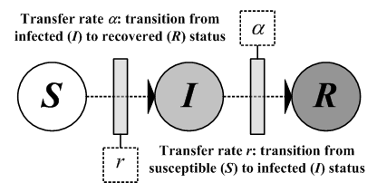
The SIR model proposed by Kermack and McKendrick (1927) remains the foundation on which most infectious disease models are formulated. As shown in Figure 2, the three letters represent the three primary states of any individual with respect to a communicable disease: Susceptible, meaning that an individual is vulnerable to infection but has not yet been infected; Infectious, meaning that an individual can infect others; and Removed, meaning that an individual has either recovered, died, or otherwise ceased to pose any further threat. During epidemic outbreaks, new infections occur because infected individuals (often referred to as infectives) come into direct contact with susceptible individuals. When such contacts take place, susceptible individuals are infected based on probabilities related to the contagiousness of the disease and their personal characteristics-some people are clearly more susceptible than others.

Figure 2
Figure 2. General SIR state transfer diagram: S, susceptible; I, infectious; R, removed

2.6
Regarding the spread of infectious diseases, a close relationship exists between social networks and individuals who come into contact with each other. The early standard version of the SIR model assumes that interactions among members of the S, I, and R subpopulations occur according to a "randomly rewired link hypothesis" (Edeletein-Keshet 1988; Kermack and McKendrick 1927). In the standard model, all individuals mingle with each other without concern for population structure. Although improbable, such a hypothesis can simplify contact factors that must be considered when formulating an epidemiological model. Based on such a hypothesis of random interaction, epidemiologists and public health specialists can easily construct an SIR model that roughly represents a range of possible transmission dynamics for epidemic outbreaks, infectious origins, and disease parameters (e.g., contagiousness, individual recovery rate, and mortality rate) based on previous infectious disease data.

2.7
Modern transportation modes and changes in lifestyles have rendered the traditional SIR model incapable of reflecting the transmission dynamics of infectious diseases. Recent statistical analyses and computational simulations of topological characteristics of social networks (e.g., local clustering, small-world, and scale-free degree distribution properties) have shown that topological characteristics of social networks exert considerable influence on transmission dynamics and spreading situations (Albert and Barabási 2002; Barabási and Albert 1999; Newman 2000; Newman and Watts 1999b; Watts 1999). In other words, the topological characteristics of social networks allow for the explanation of subtle details of infectious disease transmission that otherwise could not be understood according to a non-network approach such as the original SIR model. Small-world or scale-free networks are often integrated into SIR models to simulate interpersonal contact.

2.8
Many researchers have focused on epidemiological models with complex networks; Watts provides a thorough introduction to early work on infectious disease spreading and small-world networks in a chapter of his 1999 volume, Small Worlds: The Dynamics of Networks between Order and Randomness. Other authors who have published papers on infectious diseases and complex networks include Boots and Sasaki (1999), Dezsö and Barabási (2002), Huang et al. (2004), Keeling (1999), Kuperman and Abramson (2001), Liljeros et al. (2001), Moreno et al. (2002), Newman (2002), and Zekri and Clerc (2001). Pastor-Satorras and Vespignani (2001, 2002) observed that diseases that spread within scale-free networks do not exhibit epidemic thresholds. As part of a separate epidemic modeling approach, Newman and Watts (1999b) applied the "percolation theory" from the field of physics to study transmission dynamics and spreading consequences in SWN models. Moore and Newman (2000a, 2000b) have conducted additional research on this specific topic.

* Adjustable Small-World Network Model

3.1
We used Newman and Watts' (1999a) SWN model to construct what we believe is a more effective method for generating virtual social networks. Our proposed method uses vertex degree information for all nodes to control network connections in the form of shortcuts, in such a manner that virtual social networks that meet specific simulation or research requirements are produced. We believe our model is more practical than others because it allows for adjustments in network structure to reflect more active or conservative populations in certain regions. In other words, it produces virtual social networks that are varied in terms of interaction targets.

3.2
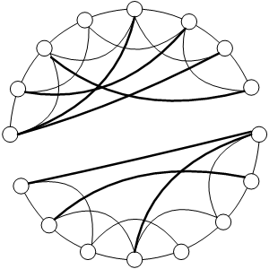
Our modified SWN model is a variation of Watts and Strogatz's (1998) original, in which SWNs consist of n-dimensional regular graphs, with each node connected to a z number of its closest nodes (Fig. 3a). There exists a probability p that each edge in a graph will be rewired, with one edge being randomly selected and reconnected to a new node (Fig. 3b).

Figure 3
Figure 3. (a) A one-dimensional regular graph with each node connected to its four adjacent nodes. (b) Watts and Strogatz's (1998) original SWN model, with four rewired edges. (c) Newman and Watts' (1999a) improved SWN model with five additional shortcuts.

3.3
As shown in Figure 4, under certain adverse circumstances Watts and Strogatz's methodology can produce breaks in a graph (Newman 2000; Newman and Watts 1999a; Wang and Chen 2003). Newman and Watts introduced a construction method that emphasizes shortcuts instead of rewiring edges (Fig. 3c). According to their method, two previously unconnected nodes are randomly selected and linked via a newly added edge, with users determining the number of new edges to be added. Newman and Watts' SWN model therefore avoids the problem of graph breakage while preserving the positive characteristic of connecting each node in the n-dimensional regular graph with 2n neighboring nodes (Wang and Chen 2003). However, since there are equal probabilities of either node being chosen when shortcuts are added, the vertex degree of each node will resemble a normal distribution, thus failing to meet the needs of users wanting to construct SWN models that utilize network structures with different distribution methods.

Figure 4
Figure 4. An example of a broken graph in Watts and Strogatz's (1998) SWN model

3.4
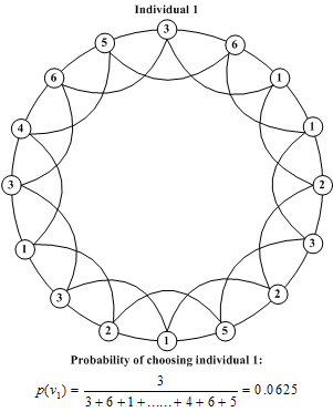
In response to restrictions in Newman and Watts' (1999a) SWN model, we propose a different construction method for the shortcut selection process. As shown in Figure 5, a user must establish the weighted vertex degree d(vi) for each node vi in the n-dimensional regular graph G before constructing a SWN model. This d(vi) value must be a real number greater than 0. Our calculations for the probability p(vi) of node vi being selected as a shortcut when a new shortcut is added are shown in Equation 1.

Equation 1 (1)

Figure 5
Figure 5. An example of calculating the probability of a node being selected

3.5
According to our construction method, the higher a node's weighted vertex degree, the higher the probability it will be selected and vice versa. When all nodes have the same weighted vertex degree, the method is identical to the SWN construction method originally proposed by Newman and Watts. For our experimental simulations (to be described in Section 6), we adopted this construction method to generate SWN models that met our specific requirements. In Experiment 1, the weighted vertex degree attribute was set according to the experiment's specific needs and the parameters used to generate the SWN model; each vertex degree attribute had a completely different setting in terms of topological structure. All of the weighted vertex degrees were set at 1, making it identical to Newman and Watts' SWN model. In our second and third experiments, the emphasis was on whether or not the distribution radius, setting, and proportion associated with specific node attribute values affected the transmission dynamics and outcomes of contagion problems. For this reason, the advantages of our proposed construction method were not fully utilized-in other words, the method was purposefully used to generate SWN models identical to that established by Newman and Watts.

3.6
The construction algorithm for our SWN model consists of the following steps:
    Step 1: for all Individuals vi in Population do loop
                Connect vi to z nearest neighbor by a von Neumann neighborhood
                Assign vertex degree ratio information d(vi) to vi
            next 
    Step 2: for 1 to shortcut number do loop
                label Generate shortcut:
                Individual va ← Choose an Individual by Probability p(va)
                Individual vb ← Choose an Individual by Probability p(vb)
                if isLinked(va, vbthen
                    goto label Generate shortcut
                end if
                Add a Shortcut between Individual va and vb
            next

* Contagion Problem Modeling

4.1
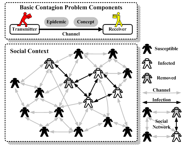
The most common (and basic) contagion problem consists of a transmitter, receiver, and channel (Blackmore 1999; Brodie 1996; Comellas et al. 2000; Lynch 1996; Marsden 1998; Shannon and Weaver 1949) (Fig. 6). For any epidemic, patients are transmitters; newly infected individuals receivers; and skin contact, insects, air and water examples of channels. Another common example used by sociologists involves filmmaking, with directors as transmitters, audiences the receivers, and actors and actresses the channels. Directors disseminate their cultural beliefs and concepts to the public via repeated screenings.

Figure 6
Figure 6. Contagion problem model

4.2
When designing our model, we took into consideration the effects of network structure, differences among individuals, and media in order to create a system in which individuals express a range of behavioral patterns. For instance, we limited the distribution of word-of-mouth rumors to small numbers of friends and neighbors within a specified time frame, but acknowledged the possibility of a rumor being spread to a wide number of recipients via email, television, radio, and the press.

4.3
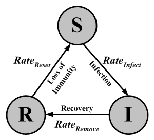
We used a simple SWN model as our social network framework because of its ability to reflect real-world interpersonal relationships. We also applied the state transfer concept of SIR models and used parameters to simulate behavioral and transformative results from interactions among individuals (Table 2). For instance, when a susceptible individual interacts with an infectious individual, a certain probability exists that the status of the former will change from S to I-a probability that we refer to as RateInfect. Eventually the probability arises that all infectious individuals are identified and placed in some form of isolation-a change in status from I to R occurring at a probability rate we refer to as RateRemove. In a typical SIR model, all R individuals are considered either dead or recovered, with recovered individuals producing antibodies that prevent them from spreading the disease to S individuals.

4.4
SIR models take on new definitions in light of epidemic cultures, rumors disseminated by word-of-mouth, and other factors associated with contagion problems. As shown in Figure 7, the susceptible state represents an openness and willingness to accept new concepts; the infectious state represents the acceptance of a specific concept and a willingness to pass it on to other individuals; and the removed state represents a loss of interest in the originally accepted concept, meaning that R individuals are not affected by the spreading behaviors of other individuals nor do they actively spread the disease or concept themselves. However, SIR models acknowledge the high possibility that an R individual will transform into an S individual-a probability that we labeled RateReset. Using fashion as an example, someone with no particular liking for hip-hop pants will start wearing them due to peer pressure, then encourage others to wear them. After a certain period of time the individual loses interest, stops wearing the pants, and doesn't notice when others continue to wear them. As more time passes, the individual has neither a strong like nor dislike of the fashion.

4.5
We also addressed the fact that SIR models are generally incapable of considering influences resulting from "differences between individuals." In our proposed model, whenever S individuals interact with I individuals, the infection rate is multiplied by weighted media factors (e.g., frequency of contact) and node attributes (e.g., individual resistance level) to determine the probability of a change in status.

4.6
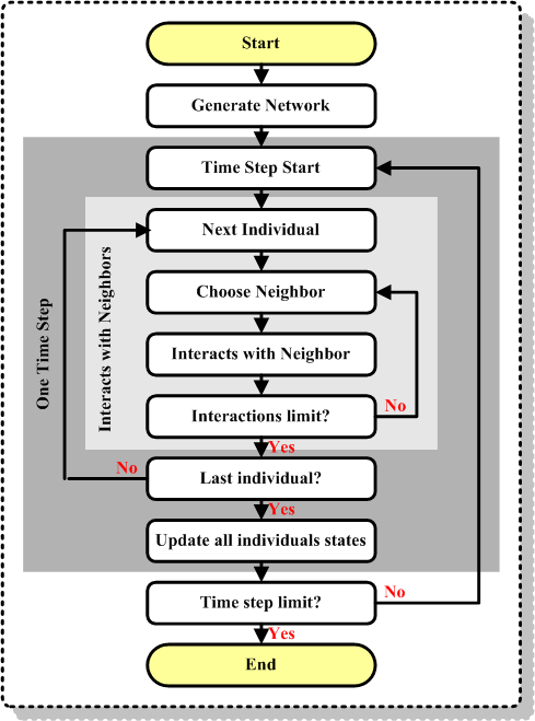
A computational simulation flowchart for our proposed model is shown in Figure 8. First, a SWN model is built using the construction method described in Section 3 prior to setting the relevant parameters and attributes of individuals involved in a problem. During a simulation, SWN individuals (nodes) take turns interacting with neighbors for specified time intervals. The randomly determined number of interactions that occur between any node and its neighbors can be fixed or variable. Individual interactions do not result in immediate influences, and simultaneous state changes only occur when all individuals in a SWN complete their interactions. Accordingly, interaction sequences do not influence interaction processes or results.

Figure 7
Figure 7. A SIR state transfer diagram showing a repetitive cycle

Figure 8
Figure 8. Simulation flowchart for a contagion problem model

4.7
The following pseudo-codes were used in our contagion problem simulation model.

    for 1 to Time Step Limit do loop

        for all Individual Ii in Population do loop
            if Interaction Mode = All then
                Interaction Limit ←     All degree numbers of Individual Ii
            else
                Interaction Limit ← 3
            end if

            for 1 to Interaction Limit do loop
                if Interaction Mode = All then
                    Individual Itarget ← Choose a neighbor of Ii by order
                else
                    Individual Itarget ← Choose a neighbor of Ii by random
                end if
                SIR(IiItarget)
            next 
        next

        for all Individual Ii in Population do loop
            if Ii.NowState = I then
                if random value r < RateRemove then
                    Ii.NextState ← R
                end if
            end if
            if Ii.NowState = R then
                if random value r < RateReset then
                    Ii.NextState ← S
                end if
            end if
        next

        comment from time t to time (t + 1)
        for all Individual Ii in Population do loop
            Ii.NowState ← Ii.NextState
        next 
    next

    procedure SIR (Individual Ia, Individual Ibis
        if Ia.NowState = I and Ib.NowState = S then
            if random value r < RateInfect ◊ Ib.Resist then
                Ib.NextState ← I
            end if
        end if
        if Ia.NowState = S and Ib.NowState = I then
            if random value r < RateInfect ◊ Ia.Resist then
                Ia.NextState ← I
            end if
        end if
    return
* Local Information Mechanisms

5.1
"Local information" is information that distinguishes certain individuals or channels from others. For example, everyone has two parents, therefore the number is considered global information. But there is considerable variation in numbers of brothers and sisters, making them a type of local information. Two primary local information categories are node-related (e.g., vertex degree and attribute) and edge-related (e.g., direction and weight). Vertex degree information represents the tendency of an individual to make friends, with extroverts having higher vertex degrees than introverts. Attribute information, which describes individual resistance to disease, is used to express divergence. Direction refers to channel direction, categorized as either uni-directional (e.g., television, radio) or bi-directional (e.g., e-mail, telephones). Weight information represents channel effect-for instance, face-to-face exchanges are viewed as having greater weight than e-mail exchanges.

5.2
The most commonly used mechanism for setting local information entails random numbers that are either normally or uniformly distributed. A second mechanism entails organizing local information according to a pre-designed pattern-for example, putting all weak (i.e., easily infected) individuals in one location versus distributing them throughout an environment. These mechanisms are applied in a manner that allows a virtual society to approximate the real world. Our goal was to observe and identify the effects of applying local information mechanisms to node-related information.

* Local Information Sensitivity Analysis Experiments

6.1
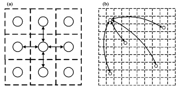
We used a variation of Newman and Watts' (1999a) SWN model (a cellular automata variation with added shortcuts) as our contagion simulation model. Since all individuals in a typical cellular automata have the same fixed number of neighbors, it can be viewed as a two-dimensional regular graph with periodic boundary conditions-for instance, a doughnut-shaped surface (Fig. 9a) (Newman 2000). If we use the method described in Section 3 to select two nodes on a two-dimensional cellular automata and to add one shortcut, the result will meet Newman and Watts' SWN model requirements for two small-world characteristics: a high degree of clustering and low degree of separation (Fig. 9b).

Figure 9
Figure 9. (a) Each individual in a cellular automata has four neighbors. (b) Each individual can have 0 to n connecting shortcuts to other randomly selected individuals

6.2
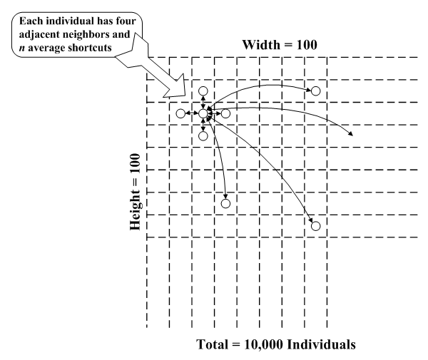
For our simulation experiments we used a 100 ◊ 100 two-dimensional cellular automata containing many shortcuts, resulting in a virtual social network consisting of 10,000 individuals (Fig. 10). This cellular automata is capable of using a von Neumann or Moore neighborhood structure; we used the von Neumann structure in our experiments because it is the preferred choice for most researchers working with low-dimensional epidemic lattice models (Moore and Newman 2000a, 2000b). This means that all individuals are connected to and interact with only four surrounding neighbors plus an undetermined number of long-distance individuals via shortcuts.

Figure 10
Figure 10. Simulation model schematic diagram

6.3
One important task was determining the appropriate number of shortcuts to add to our model. In order to mimic real-world conditions, we relied on two arguments: a) a degree of separation of approximately 6 for a world population of 6 billion (Milgram 1967), and b) a logarithmic growth relationship between the number of SWN nodes and average degree of separation (Newman 2000). For a virtual social network of 10,000 individuals, the average degree of separation is approximately 2.45, with the average individual having 21 connections: 4 connections with adjacent neighbors and 17 shortcut connections with classmates, colleagues, friends, etc.

6.4
To determine if our results and conclusions are reliable and robust and to ensure that the conclusions can be applied to any SWN model with a low degree of separation and any number of shortcuts, we built six SWN models that differed in terms of degree of separation and number of shortcuts to simulate contagion problems. All local information sensitivity analysis experiments were simulated using these models to determine consistency in the experimental results; those results indicate that our conclusions were not weakened by the two parameters.

6.5
As shown in Table 1, except for differences in the average number of node shortcuts (resulting in differences in average degree of separation), the other parameter settings for the six simulation models (cellular automata height, cellular automata width, total agent population, and neighborhood structure) were identical. The average number of shortcuts in the first model (SWN#1) was 17 and the average degree of separation 2.45, thus meeting the two conditions required to mimic real-world scenarios. The average numbers of node shortcuts in the other five simulation models were 1, 2, 4, 8 and 16, respectively; this can be expressed as 2n, with n ranging from 0 to 4. Average degrees of separation were 6.57, 5.35, 4.45, 3.59 and 3.02, also respectively-all acceptable according to recent experiments using abstract SWN models to simulate contagion problems (note models 2 and 3 in Table 1).

6.6
We therefore designated SWN#1 as the default simulation model-that is unless otherwise indicated, all results were generated by the first simulation model. According to these results, we suggest that the research conclusions are not only applicable to the SWN model represented by the first simulation model, but are also applicable to the other five simulation models, therefore being representative of most of Newman and Watts' (1999a) abstract SWN models.

Table 1: The six simulation models

Simulation ModelSWN#1*SWN#2SWN#3SWN#4SWN#5SWN#6
Average number of shortcuts per individual171 (20)2 (21)4 (22)8 (23)16 (24)
Average degree of separation2.456.575.354.453.593.02
Infection rate0.05 ~ 0.33 (based on number of interactions)
Removal rate0.9
Reset rate0.1
2-D cellular automataHeight100
Width100
Population size10,000
Neighborhood structurevon Neumann, with periodic boundary conditions

* = default simulation model.

6.7
When simulating the spread of an epidemic disease, only ten individuals were initially given I status; all others were given S status. During each time step, individuals randomly interacted with several neighbors. We experimented with two interaction modes: interactions with either three or all connected individuals. We recorded the numbers of I-state individuals after 90 iterations and compared curves generated by different settings to investigate the influences of local information. All epidemic curves discussed in this paper represent average values for 10 runs. A list of experimental parameters is presented in Table 2. Our simulation model is available as a Java application at ftp://anonymous@140.113.88.67; for source code, please contact the authors.

Table 2: Simulation model parameters

ScopeClassAttributeTypeRangeDescription
GlobalSimulation
model
Time Step LimitInteger(0, +∞)Total number of time steps during each simulation (default value = 90).
Interaction LimitInteger(0, +∞)Number of interactions between an individual and its neighbors during each time step (default value based on interaction mode value).
Interaction ModeSymbolInteraction mode: either 3 or the number of all connected individuals (default value defined according to experiment needs).
SIR modelRateInfectReal(0, 1)Infection rate
RateRemoveReal(0, 1)Removal rate (default value = 0.9).
RateResetReal(0, 1)Reset rate (default value = 0.1).
2-D cellular
automata
with
shortcuts
WidthInteger(0, +∞)Width of the 2-D cellular automata (default value = 100).
HeightInteger(0, +∞)Height of the 2-D cellular automata (default value = 100).
Population SizeInteger(0, +∞)Total numbers of individuals in the simulated society (default population size = 10,000).
NeighborhoodSymbolvon Neumann, with periodic boundary conditions
Average number of shortcutsInteger(0, +∞)Average numbers of shortcuts per individual
ExperimentRadius rReal[0, 1]Distribution radius of weak individuals (default value = 1.0).

LocalIndividualResistReal(0, +∞)Resistance to epidemic disease, trend, or idea (default value = 1.0).
Weighted
Vertex Degree
Real(0, +∞)Weighted vertex degree when choosing shortcuts (default value = 1.0).
NowStateSymbolCurrent epidemiological state
NextStateSymbolEpidemiological state in the next time step

Experiment 1: Vertex Degree

6.8
The goal of our first experiment was to identify the influence of network structure. Differences among social networks depend on the environments in which they are formed-for instance, individuals in open societies tend to have more friends than individuals in more conservative societies. Another important factor is the mix of extroverted, introverted, and in-between individuals. Sociologists are particularly interested in studying the effects of these and other factors (Chwe 2001).

6.9
We set weighted vertex degrees to meet the experimental requirement of developing different social network structures and conducted our experiments with one of three commonly used social network distribution assumptions: a) every individual's weighted vertex degree is identical, which reflects an average number of friends; b) there is a uniform distribution of weighted vertex degrees that reflects a society of 1/3 extroverts, 1/3 introverts, and 1/3 neither; and c) there is a normal distribution of weighted vertex degrees that reflects a population in which the majority of individuals are neither extroverted nor introverted, and where extreme extroverts and introverts represent small minorities.

6.10
In our initial experiment we set the weighted vertex degree for all individuals in the first assumption group at 1. The resulting social network model was very similar to Newman and Watts' (1999a) original SWN model, with the exception being the number of shortcuts. For the second group we used a randomly selected integer between 3 and 6 from the sequence of a uniform distribution as an individual's weighted vertex degree. Each value had a 25% probability of being selected, with extroverts having twice the number of opportunities of introverts for making new friends. For the third group, an integer between 1 and 9 was randomly selected from a normal distribution (M=5, SD=1) and used as an individual's weighted vertex degree. According to the principle of normal distribution, for most individuals the weighted vertex degree was 4, 5 or 6, with very few weighted vertex degrees of 1 or 9. Although each social network model had a different structure, they were very similar in terms of average degree of separation.

6.11
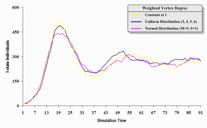
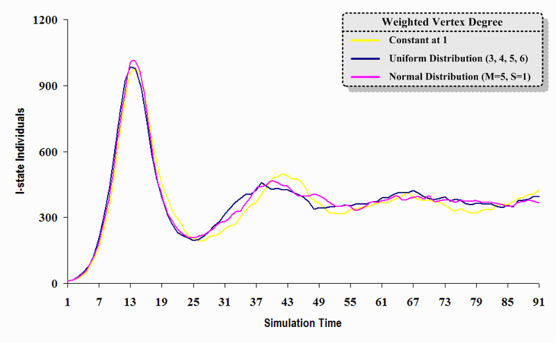
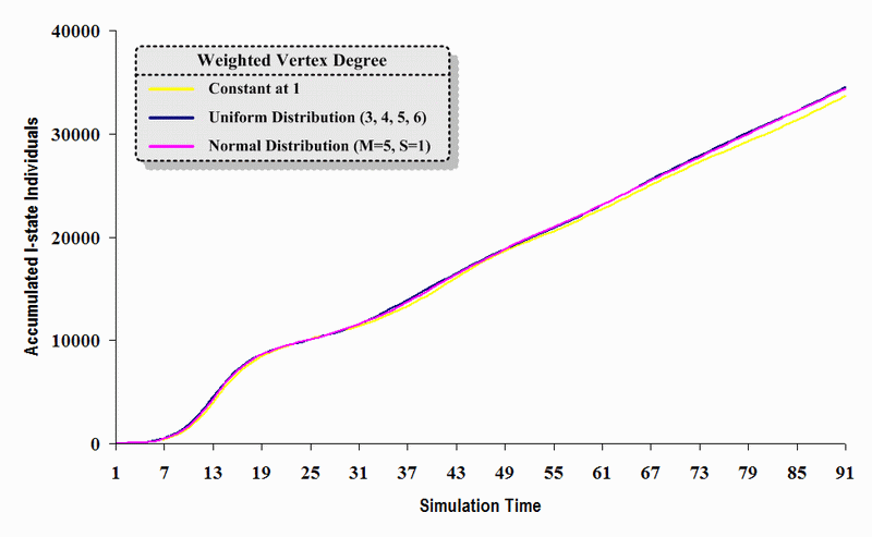
As shown in Table 3, the six simulation models generated consistent results that did not become contradictory following changes in the number of shortcuts and degrees of separation. Accordingly, we suggest that the results can be applied to various SWN models used to simulate contagion problems. To explain transmission dynamics and accumulated outcomes, we will use our results from SWN#1 (Figs. 11 and 13) and their respective cumulative sums (Figs. 12 and 14). With the exception of the maximum point for the first peak in the third epidemic curve in Figures 11 and 13, the rise and fall time points are very consistent. The cumulative sum curves for the three social network structures almost overlap, indicating a consistency of movement and fluctuation in the three curves shown in Figures 11 and 13.

6.12
In brief, the random dynamic process did not affect the overall development trend. We concluded that adding the same number of shortcuts to the three social networks used in this experiment did not exert any influence on the movement and fluctuation of the entire epidemic curve, despite differences in the regional social network structure and a slight change in the total population at the peak of the epidemic. It therefore seems unnecessary to put a great deal of effort into adjusting fine network structures when increasing the number of computational simulations. Instead, one can focus on finding appropriate global information (e.g., the number of adjacent individuals with whom connections are established or the number of shortcuts to be added).

Table 3: Experimental results using different vertex degree data with the six simulation models

Simulation ModelSWN#1SWN#2SWN#3SWN#4SWN#5SWN#6
Average accumulated number and standard deviation of infectious individuals produced by simulation model
(Mean±Std)
Interactions with 3 connected individualsInfection Rate0.30.330.330.330.330.33
Constant Mode23979
±451
11854
±588
18074
±494
21751
±582
25158
±466
26854
±403
Uniform Distribution23571
±507
12008
±459
17823
±530
21974
±514
24961
±405
26997
±418
Normal Distribution23685
±402
11896
±527
17986
±494
21917
±559
25199
±529
27079
±487
Experiment
Results
Insensitive ParameterInsensitive ParameterInsensitive ParameterInsensitive ParameterInsensitive ParameterInsensitive Parameter
Interactions with all connected individualsInfection Rate0.050.20.20.20.20.2
Constant Mode33887
±351
15913
±416
30244
±342
45147
±241
58287
±233
68492
±197
Uniform Distribution34274
±317
16286
±478
30514
±370
45220
±407
58060
±367
68340
±206
Normal Distribution34155
±266
16038
±388
30270
±463
45303
±243
58249
±343
68394
±212
Experiment ResultsInsensitive ParameterInsensitive ParameterInsensitive ParameterInsensitive ParameterInsensitive ParameterInsensitive Parameter
Conclusion:As long as small-world phenomena exist and the average degree of separation does not change, variation (e.g., constant mode, uniform distribution, and normal distribution) in the detailed topological structure exerts only a slight influence on the contagion problem transmission dynamics of SWN models.

Figure 11
Figure 11. A comparison of three sets of experimental results from the first simulation model (SWN#1) using different vertex degree data in a simulation where one individual interacts with three randomly chosen individuals per time step. Each time grid shows the resulting number of I (infectious) individuals produced by the proposed simulation model per time step.

Figure 12
Figure 12. A comparison of three sets of experimental results from the first simulation model (SWN#1) using different vertex degree data in a simulation where one individual interacts with three randomly chosen individuals per time step. Each time grid shows the accumulated number of I (infectious) individuals produced by the proposed simulation model.

Figure 13
Figure 13. A comparison of three sets of experimental results from the first simulation model (SWN#1) using different vertex degree data in a simulation where one individual interacts with all of its connected individuals per time step. Each time grid shows the resulting number of I (infectious) individuals produced by the proposed simulation model per time step

Figure 14
Figure 14. A comparison of three sets of experimental results from the first simulation model (SWN#1) using different vertex degree data in a simulation where one individual interacts with all of its connected individuals per time step. Each time grid shows the accumulated number of I (infectious) individuals produced by the proposed simulation model

6.13
One conclusion drawn from the results of the first simulation experiment is that when network components (nodes and edges) do not undergo any changes and as long as a social network exhibits small-world phenomena and an appropriate degree of separation, then fine network structure variation exerts only a slight influence on the transmission dynamics of a contagion problem. This is true whether the vertex degree of the network structure is evenly distributed (as in the SWN model generated by the first experimental setting) or unevenly distributed (second and third settings) (Figs. 11 and 13). No statistically significant effects on accumulated transmission outcomes were observed (Figs. 12 and 14).

6.14
In SWN models, network effects such as the small-world phenomena are viewed as key factors in determining transmission dynamics and outcomes regarding contagion problems. For example, the average degree of separation for the three social networks generated during our experiments using SWN#1 was 2.45, indicating that any two individuals can communicate with each other within each model as long as they are connected by 2 or 3 other individuals who transmit concepts, ideas, or materials (e.g., rumors, fashion trends, influenza, or the SARS coronavirus). As long as small-world phenomena exist and the average degree of separation does not fluctuate to a great extent, variation in the detailed topological structure does not exert a strong effect on simulation results. Conversely, when the network structure changes to such a great extent that small-world phenomena disappear, or when the average degree of separation substantially increases or decreases, simulation processes and results also change significantly.

6.15
In addition, the simulation results show that, when using SWN models to study social issues, simple arrangements can be applied for purposes of efficiency and convenience. For example, the "constant" mode (meaning every node has an identical weighted vertex degree, as in Newman and Watts' SWN model) was applied in the first setting to generate a social network. This arrangement is almost the same as those commonly used in studies of epidemics. In addition to being simple and convenient, the simulation results were identical to those generated by two arrangements of greater complexity that are considered closer to real-world conditions-that is, the vertex degree range reflects a uniform or normal distribution.

Experiment 2: Weak Individual Proportions

6.16
In our second experiment we looked at the influence of weak individuals, who constitute a certain percentage of the total population. We expected to find a range of results, since individuals have different levels of resistance to epidemic diseases and cultural influences. Since the average degree of separation between any two individuals in a SWN model is very low, we looked at the question of whether the potential for a large-scale epidemic is affected by a minority of weak individuals who are especially prone to the disease.

6.17
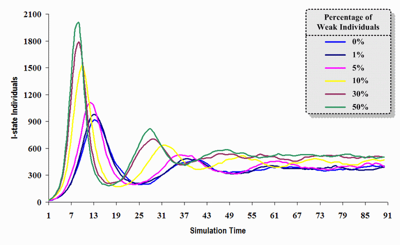
We set resistance attribute parameters to represent individual differences. For weak individuals the parameters were one-half those of ordinary individuals, meaning that weak individuals had double the probability of becoming infected. Weak and average individuals were randomly distributed throughout our virtual environments, resulting in an average weighted vertex degree of 1 for all individuals. We ran six simulations with different percentages of weak individuals: 0, 1, 5, 10, 30 and 50 percent of the entire population. When the percentage of weak individuals exceeded 50 percent, their status was changed to "average" and individuals with half the probability of infection or less were re-labeled as "strong." For this reason, we did not run simulations with percentages of weak individuals exceeding 50 percent.

6.18
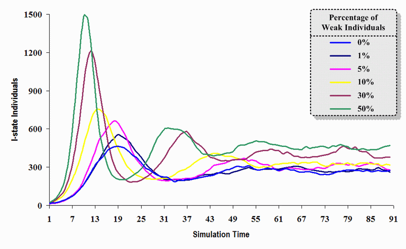
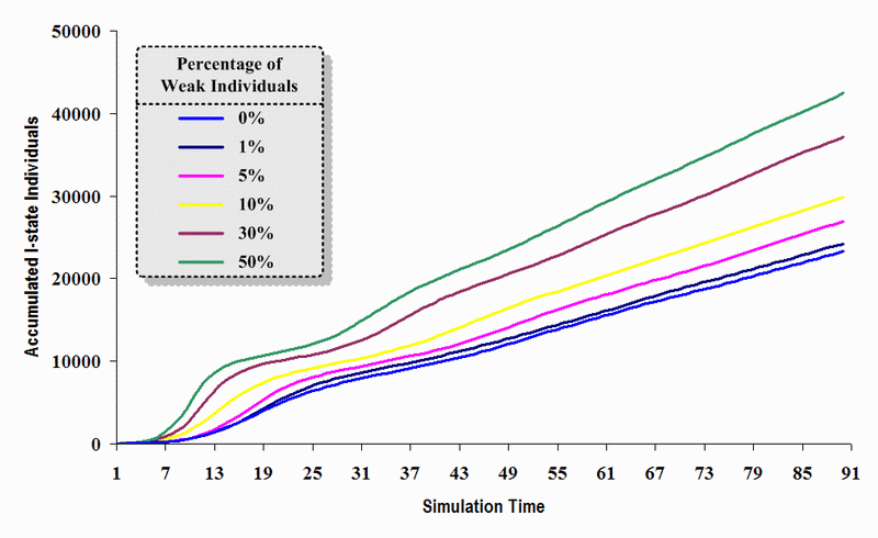
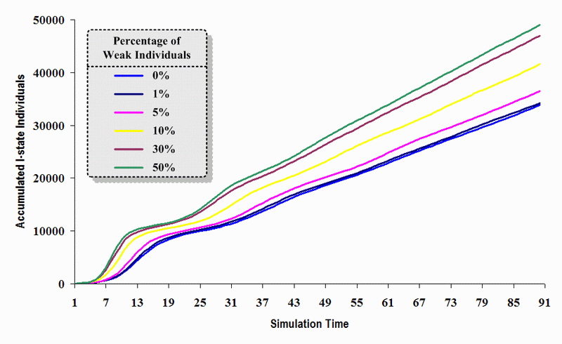
As shown in Table 4, the six simulation models generated consistent results that did not become contradictory following changes in the number of shortcuts or degree of separation. We therefore suggest that our conclusions from the second experiment can be applied to various SWN models used to simulate contagion problems. To explain the transmission dynamics and accumulated outcomes, we will use our results from SWN#1. Experimental results are shown Figures 15 and 17 and their respective cumulative sums based on time sequences are shown in Figures 16 and 18. In Figures 15 and 17, the higher the percentage of weak individuals in a population, the earlier the occurrence of the first peak and the higher its maximum point. As seen in the other two figures, the six cumulative sum curves diverged from the very beginning, with statistically significant differences noted among all six. The six epidemic curves in Figures 15 and 17 had completely different movements and fluctuations, indicating that the percentage of weak individuals exerted a significant influence on simulation results and processes. A comparison of the 0 and 1 percent curves shows that even a tiny percentage of weak individuals was enough to make a difference. These results underscore the importance of being precise when setting individual attributes for a simulation model.

Table 4: Experimental results using different proportions of weak individuals with the six simulation models

Simulation ModelSWN#1SWN#2SWN#3SWN#4SWN#5SWN#6
Average accumulated number and standard deviation of infectious individuals produced by simulation model
(Mean±Std)
Interactions with 3 connected individualsInfection Rate0.30.330.330.330.330.33
0% Weak Individuals23288
±451
12250
±346
17727
±427
22221
±428
25135
±344
26707
±409
1% Weak Individuals24032
±327
12953
±457
18329
±370
22770
±394
25546
±447
27175
±436
5% Weak Individuals26892
±517
15373
±594
21326
±423
24450
±505
27744
±523
29489
±484
10% Weak Individuals29794
±487
18951
±426
24015
±436
26849
±383
30055
±419
31894
±370
30% Weak Individuals33814
±318
27704
±532
31126
±374
34281
±454
36879
±457
38084
±506
50% Weak Individuals37124
±418
32638
±544
36517
±380
40172
±353
41165
±308
42088
±358
Experiment
Results
Sensitive ParameterSensitive ParameterSensitive ParameterSensitive ParameterSensitive ParameterSensitive Parameter

Interactions with all connected individualsInfection Rate0.050.20.20.20.10.1
0% Weak Individuals33858
±418
15576
±425
30299
±328
45073
±305
35645
±379
54764
±252
1% Weak Individuals34211
±376
16358
±391
31010
±489
45518
±215
36069
±375
55030
±168
5% Weak Individuals36478
±250
18965
±388
32787
±436
46620
±293
37761
±391
55831
±172
10% Weak Individuals41574
±328
21585
±368
34795
±327
48108
±431
39056
±487
56895
±248
30% Weak Individuals46971
±314
29448
±349
40295
±419
51986
±282
44214
±337
59804
±338
50% Weak Individuals48971
±212
34018
±354
43874
±227
54768
±224
47766
±231
61765
±234
Experiment
Results
Sensitive ParameterSensitive ParameterSensitive ParameterSensitive ParameterSensitive ParameterSensitive Parameter
Conclusion:The percentage of weak individuals exerted a significant influence on the contagion problem transmission dynamics of SWN models when small-world phenomena exist and the average degree of separation does not change.

Figure 15
Figure 15. A comparison of six sets of experimental results from the first simulation model (SWN#1) using different proportions of weak individuals in a simulation where one individual interacts with three randomly chosen individuals per time step. Each time grid shows the resulting number of I (infectious) individuals in the proposed simulation model per time step

Figure 16
Figure 16. A comparison of six sets of experimental results from the first simulation model (SWN#1) using different proportions of weak individuals in a simulation where one individual interacts with three randomly chosen individuals per time step. Each time grid shows the accumulated number of I (infectious) individuals in the proposed simulation model

Figure 17
Figure 17. A comparison of six sets of experimental results from the first simulation model (SWN#1) using different proportions of weak individuals in a simulation where one individual interacts with all of its connected individuals per time step. Each time grid shows the resulting number of I (infectious) individuals in the proposed simulation model per time step

Figure 18
Figure 18. A comparison of six sets of experimental results from the first simulation model (SWN#1) using different proportions of weak individuals in a simulation where one individual interacts with all of its connected individuals per time step. Each time grid shows the accumulated number of I (infectious) individuals in the proposed simulation model

Experiment 3: Distribution Patterns of Weak Individuals

6.19
Our goal for the third experiment was to identify the effects of the same number of weak individuals on simulations under different settings-for example, when they are centrally distributed in a specific region or evenly distributed throughout a virtual environment.

6.20
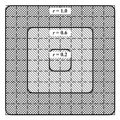
We used a radius parameter r to represent weak individual distribution ratios in one specifically defined environment relative to an entire simulation environment (Fig. 19). An r of 0 meant that all weak individuals were in close proximity to each other, an r of 1 meant that they were evenly distributed throughout a simulation environment, and an r between 0 and 1 meant that they were evenly distributed throughout a specific region within the radius parameter. When the number of weak individuals exceeded the size of the r region, the radius parameter automatically adjusted itself to the smallest possible ratio that could contain all of them. We maintained a 1 percent level of weak individuals in the total population, set the weighted vertex degree for all individuals at 1, and ran six simulations with radius parameter r values of 0 (actually 0.1), 0.2, 0.4, 0.6, 0.8 and 1.

Figure 19
Figure 19. Schematic diagram of regions covered by different radius parameters (r).

6.21
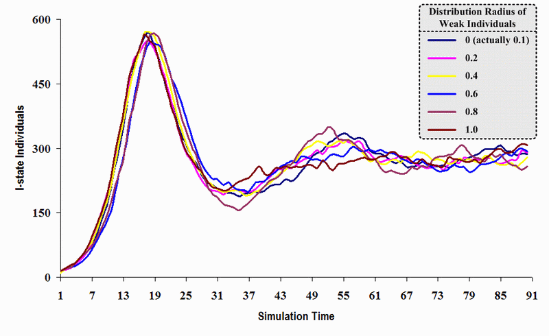
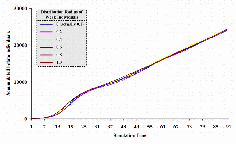
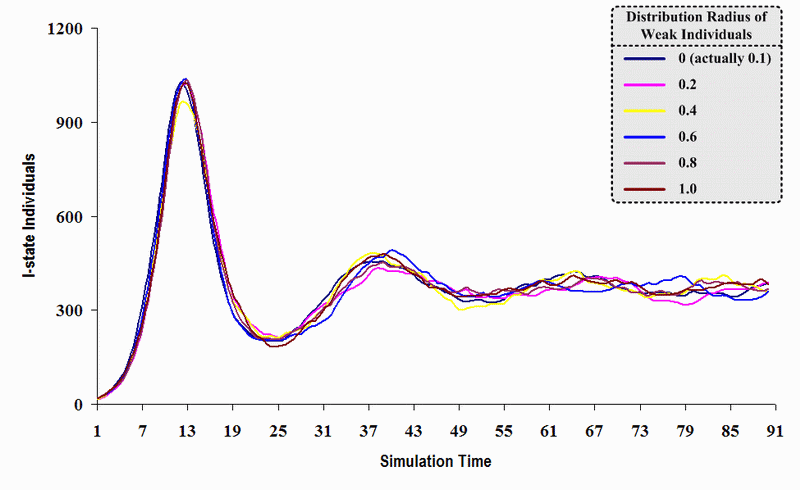
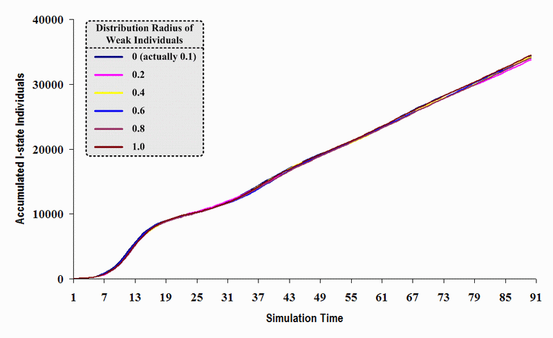
As shown in Table 5, the six simulation models generated consistent results that did not become contradictory following changes in the number of shortcuts or degree of separation. We therefore suggest that our results can be applied to various SWN models used to simulate contagion problems. To explain the transmission dynamics and accumulated outcomes, we will use the experimental results shown in Figures 20 through 23; actual results are shown in Figures 20 and 22 and their respective cumulative sums based on time sequences are shown in Figures 21 and 23. The data in Figures 20 and 22 show that with the exception of the maximum point of the first peak in the sixth epidemic curve, the time points were very consistent, with no statistically significant differences. Figures 21 and 23 show the near-overlapping of the six cumulative sum curves, indicating that the six curves in Figures 20 and 22 were very consistent in terms of movement and fluctuation. In other words, the random dynamic process of weak individual distribution did not affect development. According to these results, it is not particularly important to determine the concentrated or scattered distribution patterns of weak individuals in simulations that match or come close to matching real-world situations.

Table 5: Experimental results using different scattered radii of weak individuals with the six simulation models

Simulation ModelSWN#1SWN#2SWN#3SWN#4SWN#5SWN#6
Average accumulated number and standard deviation of infectious individuals produced by simulation model
(Mean±Std)
Interactions with 3 connected individualsInfection Rate0.30.330.330.330.330.33
Distribution Radius 0.024109
±482
12748
±513
18220
±509
22621
±435
25745
±382
27339
±218
Distribution Radius 0.224097
±344
12854
±415
18032
±408
22813
±603
25568
±327
27084
±346
Distribution Radius 0.424346
±591
12954
±535
18264
±510
22749
±294
25451
±499
27372
±241
Distribution Radius 0.623975
±227
12706
±364
18229
±310
22555
±356
25584
±505
27490
±279
Distribution Radius 0.823849
±405
12796
±518
18641
±311
22639
±583
25301
±452
27349
±364
Distribution Radius 1.024278
±419
12993
±329
18185
±367
22948
±459
25306
±506
27274
±414
Experiment
Results
Insensitive ParameterInsensitive ParameterInsensitive ParameterInsensitive ParameterInsensitive ParameterInsensitive Parameter

Interactions with all connected individualsInfection Rate0.050.20.20.20.10.1
Distribution Radius 0.034299
±271
16359
±375
30833
±480
45426
±296
35914
±373
55003
±233
Distribution Radius 0.233817
±307
16334
±395
30790
±450
45468
±248
35791
±327
54814
±251
Distribution Radius 0.434240
±255
16321
±498
31149
±296
45683
±335
35846
±338
54982
±310
Distribution Radius 0.634065
±391
16221
±398
30964
±223
45532
±275
35690
±441
54946
±201
Distribution Radius 0.834085
±249
16408
±360
31241
±417
45432
±330
35794
±355
54948
±297
Distribution Radius 1.034525
±299
16254
±338
30888
±375
45402
±337
35910
±210
54990
±168
Experiment
Results
Insensitive ParameterInsensitive ParameterInsensitive ParameterInsensitive ParameterInsensitive ParameterInsensitive Parameter
Conclusion:As long as small-world phenomena exist and the average degree of separation does not change, the distribution patterns of weak individuals do not exert any influence on the contagion problem transmission dynamics of SWN models.

Figure 20
Figure 20. A comparison of six sets of experimental results from the first simulation model (SWN#1) using different scattered radii of weak individuals in a simulation where one individual interacts with three randomly chosen individuals per time step. Each time grid shows the resulting number of I (infectious) individuals produced by the proposed simulation model per time step

Figure 21
Figure 21. A comparison of six sets of experimental results from the first simulation model (SWN#1) using different scattered radii of weak individuals in a simulation where one individual interacts with three randomly chosen individuals per time step. Each time grid shows the accumulated number of I (infectious) individuals produced by the proposed simulation model

Figure 22
Figure 22. A comparison of six sets of experimental results from the first simulation model (SWN#1) using different scattered radii of weak individuals in a simulation where one individual interacts with all of its connected individuals per time step. Each time grid shows the resulting number of I (infectious) individuals produced by the proposed simulation model per time step

Figure 23
Figure 23. A comparison of six sets of experimental results from the first simulation model (SWN#1) using different scattered radii of weak individuals in a simulation where one individual interacts with all of its connected individuals per time step. Each time grid shows the accumulated number of I (infectious) individuals produced by the proposed simulation model

6.22
Based on the combined results of the second and third experiments, we concluded that in a SWN model identical to that proposed by Newman and Watts (1999a), the two pivotal factors in determining simulation processes and results for contagion problems are a) the setting of local attribute values related to individual infectious vulnerability and resistance, and b) proportions of individuals with these particular values. Transmission dynamics and accumulated outcomes are not strongly affected by local attribute value patterns related to individual infectious vulnerability and resistance in social networks (Figs. 16 and 18).

6.23
We will offer one possible explanation for the lack of any significant effect from local attribute distribution patterns. As shown in the first experiment, the small-world phenomenon of social networks weakens the influence of some types of local information (e.g., the scattered distribution pattern in the third experiment) on contagion problems. Our calculations indicate an average degree of separation of 2.45 for SWN#1 in the three experiments-in other words, disease or concept transmission is possible when two to three people are present between any two individuals. Therefore, regardless of the distribution of weak individuals in a social network (e.g., condensed cluster or random distribution), the average degree of separation between weak and ordinary individuals is still 2.45. This means that individuals in both groups have the same probability of being infected, and the effect of a scattered pattern of weak individuals is not sufficiently strong to alter the accumulated results. In SWN model simulations of contagion problems, network effects such as small-world phenomena are considered influential global information capable of attenuating certain types of local information (e.g., the weighted vertex degrees of individuals) and influencing scattered transmission dynamic patterns and problem outcomes.

6.24
Other conclusions to be drawn from the results of the second and third experiments concern the effects of a) opinion leaders who are capable of conveying information to large numbers of individuals and therefore affect their behavior, and b) a much smaller number of indecisive individuals who regularly alter their opinions according to suggestions made by friends and relatives. Reliable simulations of infection networks require data on the percentages of opinion leaders and indecisive individuals, but not their distribution patterns.

* Conclusion

7.1
The most important conclusions from this investigation are the insignificance of the influence of vertex degree, the insignificance of weak individual distribution patterns, and the significance of weak individual percentages on contagion problems involving SWN models. We believe these results will be useful for determining simulation parameters.

7.2
Researchers who build SWN models to simulate contagion problems and social issues must focus on global variables related to network effects (e.g., small-world phenomena) and the proper setting of local information values related to individual susceptibility or resistance. On the other hand, little emphasis should be placed on the detailed topological structure of social networks (e.g., setting the weighted vertex degree) or the distribution patterns of specific local information values associated with individual susceptibility or resistance.

7.3
Regarding the influence of local information on contagion problems, we restricted our study focus to SWNs and did not consider other complex networks such as SFNs or RNs. According to recent epidemiological studies by Dezsö and Barabási (2002), Liljeros et al. (2001), and Moreno et al. (2002), certain epidemics are spread within specific types of social networks. For example, AIDS and other sexually transmitted diseases are spread within scale-free networks that exhibit both power-law degree distribution and small-world phenomena. We feel that a logical next step will be to apply our proposed simulation model (including a modified SIR model and adjustable SWN models) to explore the influence of local information in complex networks on the transmission dynamics and outcomes of contagion problems.

7.4
Our future plans include an investigation of edge-related local information, which can be divided into two categories: a) one-way versus bilateral interactions between individuals, and b) having attributes that reflect interaction details between two individuals (e.g., frequency of contact and ease of transmission).

* Acknowledgement

This work was supported in part by National Science Council, Taiwan, Republic of China under grant NSC 92-2524-S-009-004 and NSC 93-2520-S-009-003.

* References

ALBERT R and Barabási A-L (2002) Statistical Mechanics of Complex Networks. Review of Modern Physics, 74, pp. 47-91.

ALBERT R, Jeong H, and Barabási A-L (1999) Diameter of the World Wide Web. Nature, 401, pp. 130-131.

BARABÁSI A-L, Albert R, and Jeong H (1999) Mean-field Theory for Scale-Free Random Networks. Physica A, 272, pp. 173-187.

BARABÁSI A-L and Albert R (1999) Emergence of Scaling in Random Networks. Science, 286(5439), pp. 509-512.

BLACKMORE S (1999) The Meme Machine. Oxford: Oxford University press.

BOOTS M and Sasaki A (1999) "Small Worlds" and the Evolution of Virulence: Infection Occurs Locally and at a Distance. Proceedings of the Royal Society of London, Series B, 266(1432), pp. 1933-1938.

BRODIE R (1996) Virus of the Mind: The New Science of the Meme. Seattle, WA: Integral Press.

CHWE M S Y (2001) Rational Ritual: Culture, Coordination, and Common Knowledge. Princeton NJ: Princeton University Press.

COMELLAS F, Ozon J, and Peters J G (2000) Deterministic Small-World Communication Networks. Information Processing Letters, 76(1-2), pp. 83-90.

DEZSÖ Z and Barabási A-L (2002) Halting Viruses in Scale-Free Networks. Physical Review E, 65(5 Pt 2). 055103.

EDELETEIN-KESHET L (1988) Mathematical Models in Biology. Random House, New York.

ERDÖS P and Renyi A (1959) On the Evolution of Random Graphs. Publication of the Mathematical Institute of the Hungarian Academy of Science, 5, pp. 17-60.

FALOUTSOS M, Faloutsos P, and Faloutsos C (1999) On Power-law Relationships of the Internet Topology. Computer Communications Review, 29, pp. 251-263.

HUANG C Y, Sun C T, Hsieh J L, and Lin H (2004) Simulating SARS: Small-World Epidemiological Modeling and Public Health Policy Assessments. Journal of Artificial Societies and Social Simulation, 7(4), https://www.jasss.org/7/4/2.html.

KEELING M J (1999) The Effects of Local Spatial Structure on Epidemiological Invasions. Proceedings of the Royal Society of London, 266, pp. 859-867.

KERMACK W O and McKendrick A G (1927) Contributions to the Mathematical Theory of Epidemics. Proceedings of the Royal Society of London, Series A, 115, pp. 700-721.

KUPERMAN M and Abramson G (2001) Small World Effect in an Epidemiological Model. Physical Review Letters, 86(13), pp. 2909-2912.

LILJEROS F, Edling C R, Amaral L A N, Stanley H E, and Aberg Y (2001) The Web of Human Sexual Contacts, Nature, 411, pp. 907-908.

LYNCH A (1996) Thought Contagion: How Belief Spreads Through Society: The New Science of Memes. New York, NY: Basic Books.

MARSDEN P (1998) Memetics and Social Contagion: Two Sides of the Same Coin? Journal of Memetics - Evolutionary Models of Information Transmission, 2(2), pp. 171-185.

MEDINA A, Matta I, and Byers J (2000) On the Origin of Power-laws in Internet Topologies. ACM Computer Communications Review, 30(2), pp. 18-28.

MILGRAM S (1967) The Small World Problem. Psychology Today, 2, pp. 60-67.

MOORE C and Newman M E J (2000a) Epidemics and Percolation in Small-world Networks. Physical Review E, 61(5 Pt B), pp. 5678-5682.

MOORE C and Newman M E J (2000b) Exact Solution of Site and Bond Percolation on Small World Networks. Physical Review E, 62, pp. 7059-7064.

MORENO Y, Pastor-Satorras R, and Vespignani A (2002) Epidemic outbreaks in complex heterogeneous networks. European Physical Journal B, 26(4), pp. 521-529.

NEWMAN M E J and Watts D J (1999a) Renormalization Group Analysis of the Small-world Network Model. Physics Letters A, 263, pp. 341-346.

NEWMAN M E J and Watts D J (1999b) Scaling and Percolation in the Small-World Network Model. Physical Review E, 60(6 Pt B), pp. 7332-7342.

NEWMAN M E J (2000) Models of the Small World: A Review. Journal of Statistical Physics, 101, pp. 819-841.

NEWMAN M E J (2002) Spread of epidemic disease on networks. Physical Review E, 66 (1 Pt 2). 016128.

PASTOR-SATORRAS R and Vespignani A (2001) Epdiemic Spreading in Scale-Free Networks. Physical Review Letter, 86, pp. 3200-3203.

PASTOR-SATORRAS R and Vespignani A (2002) Epidemics and Immunization in Scale-Free Networks. In Bornholdt S and Schuster H G (eds.), Handbook of Graphs and Networks: From the Genome to the Internet, Wiley-VCH, Berlin.

SHANNON CE and Weaver W (1949) The Mathematical Theory of Communication. Urbana, IL: University of Illinois Press.

TSIMRING L S and Huerta R (2003) Modeling of Contact Tracing in Social Networks. Physica A, 325, pp. 33-39.

WANG X F and Chen G (2003) Complex Networks: Small-World, Scale-Free and Beyond. IEEE Circuits and Systems Magazine, First Quarter, pp. 6-20.

WATTS D J (1999) Small Worlds: The Dynamics of Networks between Order and Randomness. Princeton NJ: Princeton University Press.

WATTS D J and Strogatz S H (1998) Collective Dynamics of 'Small-world' Networks. Nature, 393(6684), pp. 440-442.

ZANETTE D H (2003) Models of Social Processes on Small-World Networks. AIP Conference Proceeding, 658, pp. 187-203.

ZEKRI N and Clerc J P (2001) Statistical and Dynamical Study of Disease Propagation in a Small World Network. Physical Review E, 64(5), 056115.

----

ButtonReturn to Contents of this issue

© Copyright Journal of Artificial Societies and Social Simulation, [2005]